GRASS: Trimming Stragglers in Approximation Analytics
←
→
Page content transcription
If your browser does not render page correctly, please read the page content below
GRASS: Trimming Stragglers in Approximation Analytics
 Ganesh Ananthanarayanan1 , Michael Chien-Chun Hung2 , Xiaoqi Ren3 , Ion Stoica1 , Adam Wierman3 , Minlan Yu2
     1
         University of California, Berkeley, 2 University of Southern California, 3 California Institute of Technology

                         Abstract                                  even if only on part of the dataset, is more important than
   In big data analytics timely results, even if based on          processing the entire data. These jobs tend to have ap-
only part of the data, are often good enough. For this             proximation bounds on two dimensions—deadline and
reason, approximation jobs, which have deadline or er-             error [7]. Deadline-bound jobs strive to maximize the
ror bounds and require only a subset of their tasks to             accuracy of their result within a specified time deadline.
complete, are projected to dominate big data workloads.            Error-bound jobs, on the other hand, strive to minimize
Straggler tasks are an important hurdle when designing             the time taken to reach a specified error limit in the re-
approximate data analytic frameworks, and the widely               sult. Typically, approximation jobs are launched on a
adopted approach to deal with them is speculative ex-              large dataset and require only a subset of their tasks to
ecution. In this paper, we present GRASS, which care-              finish based on the bound [8, 9, 10].
fully uses speculation to mitigate the impact of stragglers           Our focus is on the problem of speculation for approx-
in approximation jobs. The design of GRASS is based                imation jobs.1 Traditional speculation techniques for
on first principles analysis of the impact of speculative          straggler mitigation face a fundamental limitation when
copies. GRASS delicately balances immediacy of im-                 dealing with approximation jobs, since they do not take
proving the approximation goal with the long term impli-           into account approximation bounds. Ideally, when the
cations of using extra resources for speculation. Evalua-          job has many more tasks than compute slots, we want to
tions with production workloads from Facebook and Mi-              prioritize those tasks that are likely to complete within
crosoft Bing in an EC2 cluster of 200 nodes shows that             the deadline or those that contribute the earliest to meet-
GRASS increases accuracy of deadline-bound jobs by                 ing the error bound. By not considering the approxi-
47% and speeds up error-bound jobs by 38%. GRASS’s                 mation bounds, state-of-the-art straggler mitigation tech-
design also speeds up exact computations, making it a              niques in production clusters at Facebook and Bing fall
unified solution for straggler mitigation.                         significantly short of optimal mitigation. They are 48%
                                                                   lower in average accuracy for deadline-bound jobs and
                                                                   40% higher in average duration of error-bound jobs.
1   Introduction                                                      Optimally prioritizing tasks of a job to slots is a classic
                                                                   scheduling problem with known heuristics [11, 12, 13].
Large scale data analytics frameworks automatically                These heuristics, unfortunately, do not directly carry
compose jobs operating on large data sets into many                over to our scenario for the following reasons. First,
small tasks and execute them in parallel on compute                they calculate the optimal ordering statically. Straggling
slots on different machines. A key feature catalyzing the          of tasks, on the other hand, is unpredictable and ne-
widespread adoption of these frameworks is their abil-             cessitates dynamic modification of the priority ordering
ity to guard against failures of tasks, both when tasks            of tasks according to the approximation bounds. Sec-
fail outright as well as when they run slower than the             ond, and most importantly, traditional prioritization tech-
other tasks of the job. Dealing with the latter, referred to       niques assign tasks to slots assuming every task to oc-
as stragglers, is a crucial design component that has re-          cupy only one slot. Spawning a speculative copy, how-
ceived widespread attention across prior studies [1, 2, 3].        ever, leads to the same task using two (or multiple)
   The dominant technique to mitigate stragglers                   slots simultaneously. Hence, this distills our challenge
is speculation—launching speculative copies for the                to achieving the approximation bounds by dynamically
slower tasks, where a speculative copy is simply a dupli-          weighing the gains due to speculation against the cost of
cate of the original task. It then becomes a race between          using extra resources for speculation.
the original and the speculative copies. Such techniques
                                                                      Scheduling a speculative copy helps make immediate
are state-of-the-art and deployed in production clusters
                                                                   progress by finishing a task faster. However, while not
at Facebook and Microsoft Bing, thereby significantly
                                                                   scheduling a speculative copy results in the task run-
speeding up jobs. The focus of this paper is on specula-
                                                                   ning slower, many more tasks may be completed using
tion for an emerging class of jobs: approximation jobs.
   Approximation jobs are starting to see considerable                1 Note that an error-bound job with error of zero is the same as an
interest in data analytics clusters [4, 5, 6]. These jobs          exact job that requires all its tasks to complete. Hence, by focusing on
are based on the premise that providing a timely result,           approximation jobs, we automatically subsume exact computations.

                                                               1
the saved slot. To understand this opportunity cost, con- 2.1 Approximation Jobs
sider a cluster with one unoccupied slot and a straggler
Increasingly, with the deluge of data, analytics applica-
task. Letting the straggler complete takes five more time
tions no longer require processing entire datasets. In-
units while a new copy of it would take four time units.
stead, they choose to tradeoff accuracy for response time.
Scheduling a speculative copy for this straggler speeds it
Approximate results obtained early from just part of the
up by one time unit, however, if we were not to, that slot
dataset are often good enough [4, 6, 5]. Approximation
could finish another task (taking five time units too).
is explored across two dimensions—time for obtaining
This simple intuition of opportunity cost forms the ba- the result (deadline) and error in the result [7].
sis for our two design proposals. First, Greedy Spec-
ulative (GS) scheduling is an algorithm that greedily • Deadline-bound jobs strive to maximize the accu-
picks the task to schedule next (original or speculative) racy of their result within a specified time limit.
that most improves the approximation goal at that point. Such jobs are common in real-time advertisement
Second, Resource Aware Speculative (RAS) scheduling systems and web search engines. Generally, the job
considers the opportunity cost and schedules a specula- is spawned on a large dataset and accuracy is pro-
tive copy only if doing so saves both time and resources. portional to the fraction of data processed [8, 9, 10]
These two designs are motivated by first principles (or tasks completed, for ease of exposition).
analysis within the context of a theoretical model for • Error-bound jobs strive to minimize the time taken
studying speculative scheduling. An important guideline to reach a specified error limit in the result. Again,
from our model is that the value of being greedy (GS) accuracy is measured in the amount of data pro-
increases for smaller jobs while considering opportunity cessed (or tasks completed). Error-bound jobs are
cost of speculation (RAS) helps for larger jobs. As our used in scenarios where the value in reducing the
model is generic, a nice aspect is that the guideline holds error below a limit is marginal, e.g., counting of the
not only for approximation jobs but also for exact jobs number of cars crossing a section of a road to the
that require all their tasks to complete. nearest thousand is sufficient for many purposes.
We use the above guideline to dynamically combine Approximation jobs require schedulers to prioritize
GS and RAS, which we call GRASS. At the beginning the appropriate subset of their tasks depending on the
of a job’s execution, GRASS uses RAS for scheduling deadline or error bound. Prioritization is important for
tasks. Then, as the job gets close to its approximation two reasons. First, due to cluster heterogeneities [2, 3,
bound, it switches to GS, since our theoretical model 16], tasks take different durations even if assigned the
suggests that the opportunity cost of speculation dimin- same amount of work. Second, jobs are often multi-
ishes with fewer unscheduled tasks in the job. GRASS waved, i.e., their number of tasks is much more than
learns the point to switch from RAS to GS using job and available compute slots [17], thereby they run only a
cluster characteristics. fraction of their tasks at a time. The trend of multi-waved
We demonstrate the generality of GRASS by imple- jobs is only expected to grow with smaller tasks [18].
menting it in both Hadoop [14] (for batch jobs) and
Spark [15] (for interactive jobs). We evaluate GRASS
using production workloads from Facebook and Bing on 2.2 Challenges
an EC2 cluster with 200 machines. GRASS increases The main challenge in prioritizing tasks of approxima-
accuracy of deadline-bound jobs by 47% and speeds up tion jobs arises due to some of them straggling. Even
error-bound jobs by 38% compared to state-of-the-art after applying many proactive techniques, in production
straggler mitigation techniques deployed in these clus- clusters in Facebook and Microsoft Bing, the average
ters (LATE [2] and Mantri [1]). In fact, GRASS results job’s slowest task is eight times slower than the median.2
in near-optimal performance. In addition, GRASS also Further, it is difficult to model all the complex interac-
speeds up exact jobs, that require all their tasks to com- tions in clusters to prevent stragglers [3, 19].
plete, by 34%. Thus, it is a unified speculation solution The widely adopted technique to deal with straggler
for both approximation as well as exact computations. tasks is speculation. This is a reactive technique that
spawns speculative copies for tasks deemed to be strag-
gling. The earliest among the original and speculative
2 Challenges and Opportunities copies is picked while the rest are killed. While schedul-
ing a speculative copy makes the task finish faster and
thereby increases accuracy, they also compete for com-
Before presenting our system design, it is important to
pute slots with the unscheduled tasks.
understand the challenges and opportunities for speculat-
ing straggler tasks in the context of approximation jobs. 2 Task durations are normalized by their input sizes.
2Therefore, our problem is to dynamically prioritize
tasks based on the deadline/error-bound while choosing
between speculative copies for stragglers and unsched-
uled tasks. This problem is, unfortunately, NP-Hard and
devising good heuristics (i.e., with good approximation
factors) is an open theoretical problem.
2.3 Potential Gains
Given the challenges posed by stragglers discussed Figure 1: GS and RAS for a deadline-bound job with 9
above, it is not surprising that the potential gains from tasks. The trem and tnew values are when T2 finishes. The
mitigating their impact are significant. To highlight this example illustrates deadline values of 3 and 6 time units.
we use a simulator with an optimal bin-packing sched-
uler. Our baselines are the the state-of-the-art mitigation
strategies (LATE [2] and Mantri [1]) in the production in the system, and thus maximize the number of tasks
clusters. Optimally prioritizing the tasks while correctly completed, at all points of time among the class of non-
balancing between speculative copies and unscheduled preemptive policies [11, 12]. Thus, without speculation,
tasks presents the following potential gains. Deadline- SJF finishes the most tasks before the deadline.
bound jobs improve their accuracy by 48% and 44%, in If one extends this idea to the case where speculation
the Facebook and Bing traces, respectively. Error-bound is allowed, then a natural approach is to allow the tasks
jobs speed up by 32% and 40%. We next develop an that are currently running to also be placed in the queue,
online heuristic to achieve these gains. and to choose the task with the smallest size, i.e., tnew
(requiring, of course, that the task can finish before the
deadline). Then, if the chosen task has a copy currently
3 Speculation Algorithm Design running, we check that the new speculative copy being
The key choice made by a cluster scheduling algorithm considered provides a benefit, i.e., tnew < trem . So, the
is to pick the next task to schedule given a vacant slot. next task to run is still chosen according to SJF, only
Traditionally, this choice is made among the set of tasks now speculative copies are also considered. We term this
that are queued; however when speculation is allowed, policy Greedy Speculative (GS) scheduling, because it
the choice also includes speculative copies of tasks that picks the next task to schedule greedily, i.e., the one that
are already running. This extra flexibility means that will finish the quickest, and thus improve the accuracy
a design must determine a prioritization that carefully the earliest at present.
weighs the gains from speculation against the cost of Figure 1 (left) presents an illustration of GS for a sim-
extra resources while still meeting the approximation ple job with nine tasks and two concurrent slots. Tasks
goals. Thus, we first focus on tradeoffs in the design T1 and T2 are scheduled first, and when T2 finishes, the
of the speculation policy. Specifically, using both small trem and tnew values are as indicated. At this point, GS
examples and analytic modeling we motivate the use of schedules T3 next as it is the one with the lowest tnew ,
two simple heuristics, Greedy Speculative (GS) schedul- and so forth. Assuming the deadline was set to 6 time
ing and Resource Aware Speculative (RAS) scheduling units, the obtained accuracy is 79 (or 7 completed tasks).
that together make up the core of GRASS. Picking the earliest task to schedule next is often op-
timal when a job has no unscheduled tasks (i.e., either
single-waved jobs or the last wave of a multi-waved job).
3.1 Speculation Alternatives However, when there are unscheduled tasks it is less
For simplicity, we first introduce GS and RAS in the clear. For example, in Figure 1 (right) if we schedule
context of deadline-bound jobs and then briefly describe a speculative copy of T1 when T2 finished, instead of
how they can be adapted to error-bound jobs. T3, 8 tasks finish by the deadline of 6 time units.
The previous example highlights that running a spec-
3.1.1 Deadline-bound Jobs ulative copy has resource implications which are impor-
tant to consider. If the speculative copy finishes early,
If speculation was not allowed, there is a natural, well- both slots (of the speculative copy and the original) be-
understood policy for the case of deadline-bound jobs: come available sooner to start the other tasks. This op-
Shortest Job First (SJF), which schedules the task with portunity cost of speculation is an important tradeoff to
the smallest processing time. In many settings, SJF can consider, and leads to the second policy we consider: Re-
be proven to minimize the number of incomplete tasks source Aware Speculative (RAS) scheduling.
31: procedure D EADLINE(hTaski T , float δ, bool OC) 1: procedure E RROR(hTaski T , float , bool OC)
. OC = 1 → use RAS; 0 → use GS . OC = 1 → use RAS; 0 → use GS
2: if OC then . Error is in #tasks
3: for each Task t in T do 2: for each Task t in T do
4: if t.running then t.duration = min(t.trem , t.tnew )
t.saving = t.c ×t.trem − (t.c+1) × tnew 3: if OC then
. PRUNING STAGE 4: if t.running then
δ’ ← Remaining Time to δ t.saving = t.c ×t.trem − (t.c+1) × tnew
hTaskiΓ ← φ . PRUNING STAGE
5: for each Task t in T do SortAscending(T , “duration”)
6: if t.tnew > δ’ then continue . Exceeds deadline hTaskiΓ ← φ
7: if OC then 5: for each Task t in T [0 : T .count() (1 − )] do
8: if t.saving > 0 then Γ.add(t) . Earliest tasks
9: else 6: if OC then
10: if t.running then 7: if t.saving > 0 then Γ.add(t)
11: if t.tnew < t.trem then Γ.add(t) 8: else
12: else Γ.add(t) 9: if t.running then
. SELECTION STAGE 10: if t.tnew < t.trem then Γ.add(t)
13: if Γ 6= null then 11: else Γ.add(t)
14: if OC then SortDescending(Γ, “saving”) . SELECTION STAGE
15: else SortAscending(Γ, tnew ) 12: if Γ 6= null then
return Γ.first() 13: if OC then SortDescending(Γ, “saving”)
14: else SortDescending(Γ, trem )
Pseudocode 1: GS and RAS algorithms for deadline-
return Γ.first()
bound jobs (deadline of δ). T is the set of unfinished tasks
with the following fields per task: trem , tnew , and a boolean Pseudocode 2: GS and RAS speculation algorithms for
“running” to denote if a copy of it is currently executing. error-bound jobs (error-bound of ). T is the set of un-
RAS is used when OC is set. At default, both algorithms finished tasks with the following fields per task: trem , tnew ,
schedule the task with the lowest tnew within the deadline. and a boolean “running” to denote if a copy of it is cur-
rently executing. The trem of the task is the minimum of all
its running copies. RAS is used when OC is set. At default,
To account for the opportunity cost of scheduling a both algorithms schedule the task with the highest trem .
speculative copy, RAS speculates only if it saves both
time and resources. Thus, not only must tnew be less
than trem to spawn a speculative copy but the sum of the portant factor, which we discuss later in §4.1, is the esti-
resources used by the speculative and original copies, mation accuracy of trem and tnew .
when running simultaneously, must be less than letting Pseudocode 1 describes the details of GS and RAS.
just the original copy finish. In other words, for a task The set T consists of all the running and unscheduled
with c running copies, its resource savings, defined as tasks of the jobs. There are two stages in the scheduling
c × trem − (c + 1) × tnew , must be positive. process: (i) Pruning Stage: In this stage (lines 5 − 12),
By accounting for the opportunity cost of resources, tasks that are not slated to complete by the deadline are
RAS can out-perform GS in many cases. As mentioned removed from consideration. Further, GS removes those
earlier, in Figure 1 (right) where RAS achieves an ac- tasks whose speculative copy is not expected to finish
curacy of 89 versus GS’s 79 in the deadline of 6 time earlier than the running copy. RAS removes those tasks
units. This improvement comes because, when T2 fin- which do not save on resources by speculation. (ii) Se-
ishes, speculating on T1 saves 1 unit of resource. lection Stage: From the pruned set, GS picks the task
However, RAS is not uniformly better than GS. In par- with the lowest tnew while RAS picks the task with the
ticular, RAS’s cautious approach can backfire if it over- highest resource savings (lines 13 − 15).
estimates the opportunity cost. In the same example in
Figure 1, if the deadline of the job were reduced from 3.1.2 Error-bound Jobs
6 time units to 3 time units instead, GS performs bet-
ter than RAS. At the end of 3 time units, GS has led to Though error-bound jobs require a different form of
three completed tasks while RAS has little to show for prioritization than deadline-bound jobs, the speculative
its resource gains by speculating T1. core of the GS and RAS algorithms are again quite natu-
As the example alludes to, the value of the deadline ral. Specifically, the goal of error-bound jobs is to mini-
and the number of waves are two important factors im- mize the makespan of the tasks needed to achieve the er-
pact whether GS or RAS is a better choice. A third im- ror limit. Thus, instead of SJF, Longest Job First (LJF) is
4Processing Time/Optimal
GS RAS
5 waves
Hill estimate of β
4 1.1 4 waves
3 waves
3 2 waves
1 waves
2 1.05
β = 1.259
1
0 1
1 2 3 4 1 2 3 4 5
order statistics x 10
6 ω
Figure 3: Hill plot of Face- Figure 4: Near-optimality
book task durations. of GS & RAS under Pareto
task durations (β = 1.259).
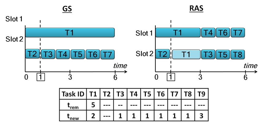
Figure 2: GS and RAS for error-bound job with 6 tasks.
The trem and tnew values are when T2 finishes. The example
illustrates error limit of 40% (3 tasks) and 20% (4 tasks). lation is only valuable if task durations are extremely
heavy tailed, e.g., Pareto with infinite variance (i.e., with
shape parameter β < 2). In this case, it is optimal to
the natural prioritization of tasks. In particular, LJF min-
speculate conservatively, using ≤ 2 copies of a task.
imizes the makespan among the class of non-preemptive
policies in many settings [11, 12]. This again represents Task durations are indeed heavy-tailed for the Facebook
a “greedy” prioritization for this setting. and Bing traces, as illustrated by the Hill plot3 in Figure
Despite the above change to the prioritization of which 3. Task durations have a Pareto tail with shape parameter
task to schedule, the form of GS and RAS remain the β = 1.259. While both GS and RAS speculate during
same as in the case of deadline-bound jobs. In particular, early waves, RAS is more conservative than GS and thus
speculative copies are evaluated in the same manner, e.g., outperforms it during early waves.
RAS’s criterion is still to pick the task whose specula-
tion leads to the highest resource savings. Pseudocode 2 Guideline 2 During the final wave of a job, speculate
presents the details. The pruning stage (lines 5 − 11) aggressively to fully utilize the allotted capacity.
will remove from consideration those tasks that are not Even if all tasks are currently scheduled, if a slot be-
the earliest to contribute to the desired error bound. The comes available it should be filled with a speculative
list of earliest tasks is based on the effective duration of copy. Note that both GS and RAS do this to some extent,
every task, i.e., the minimum of trem and tnew . During se- but since GS speculates more aggressively than RAS it
lection (lines 12−14), GS picks the task with the highest outperforms RAS during the final wave.
trem while RAS picks the task with the highest saving.
Figure 2 presents an illustration of GS and RAS for an Guideline 3 For jobs that require more than two waves
error-bound job with 6 tasks and 3 compute slots. The RAS is near-optimal, while for jobs that require fewer
trem and tnew values are at 5 time units. GS decides to than two waves GS is near-optimal.
launch a copy of T3 as it has the highest trem . RAS con-
servatively avoids doing so. Consequently, when the er- To make this point more salient, consider an arbitrary
ror limit is high (say, 40%) GS is quicker, but RAS is speculative policy that waits until a task has run ω time
better when the limit decreases (to, say, 20%). before starting a speculative copy (see §A). GS and
RAS correspond to particular rules for choosing ω. To
translate them into the model, we define tnew = E[τ ]
3.2 Contrasting GS and RAS
and trem = E[τ − ω|τ > ω], where τ is a random
To this point, we have seen that GS and RAS are two nat- task size. Then, under GS, ω is the time when E[τ ] =
ural approaches for integrating speculation into a clus- E[τ − ω|τ > ω], and, under RAS, ω is the time when
ter scheduler for approximation jobs. However, the ex- 2E[τ ] = E[τ − ω|τ > ω].
amples we have considered highlight that neither of GS Figure 4 shows the ratio of the response time normal-
or RAS is uniformly better. In order to develop a bet- ized to the optimal duration for jobs of differing num-
ter understanding of these two algorithms, as well as bers of waves, with parameter ω ∈ [0, 5]. GS and RAS
other possible alternatives, we have developed a sim- are shown via vertical lines. The figure shows that nei-
ple analytic model for speculation in approximation jobs. ther GS or RAS is universally optimal, but each is near-
The model assumes wave-based scheduling and constant optimal over a range of job types.
wave-width for a job (see §A for details along with for- 3 A Hill plot provides a more robust estimation of Pareto distribu-
mal results). For readability, here we present only the tions than regression on a log-log plot [20]. The fact that the curve is
three major guidelines from our analysis. flat over a large range of scales (on the x-axis), but not all scales, indi-
cates that the whole distribution is likely not Pareto, but that the tail of
Guideline 1 During the early waves of a job, specu- the distribution is well-approximated by a Pareto tail.
5This motivates a system design that starts using RAS checks by using the remaining work at any point (mea-
for early waves and then switches to GS for the final sured in time remaining or tasks to complete) to calculate
two waves. However, in practice, identifying the “final the effect of switching to GS. It steps through all possi-
two waves” is difficult since this requires predicting how ble points in its remaining work at which it could switch
many tasks will complete either before the deadline or and estimates the optimal point using job samples of ap-
error limit is reached. Hence, we interpret this guideline propriate sizes. It continues with RAS until the optimal
as when the deadline is loose or the error limit is low, switching point turns out to be at present. The above
then RAS is better, while otherwise GS performs better, calculation for the optimal switching point is performed
mimicking the intuition from the examples in §3.1. periodically during the job’s execution.
The optimal switching point changes with time be-
cause the size of the job alone is insufficient for the
4 GRASS Speculation Algorithm calculation. Even jobs of comparable size might have
different number of waves depending on the number of
In this section, we build our speculation algorithm called
available slots. Therefore, we augment our samples of
GRASS.4 Our theoretical analysis summarized in §3.2
job performance with the number of waves of execution,
highlights that it is desirable to use RAS during the early
simply approximated using current cluster utilization.
waves of jobs and GS during the final two waves. A sim-
Finally, estimation accuracy of trem and tnew also de-
ple strawman solution to achieve this would be as fol-
cides the optimal switching point. RAS’s cautious ap-
lows. For deadline-bound jobs, switch from RAS to GS
proach of considering the opportunity cost of speculat-
when the time to the deadline is sufficient for at most two
ing a task is valuable when task estimates are erroneous.
waves of tasks. Similarly, for error-bound jobs, switch
In fact, at low estimation accuracies (along with certain
when the number of (unique) scheduled tasks needed to
values of utilization and deadline/error-bound), it is bet-
satisfy the error-bound makes up two waves.
ter to not switch to GS at all and employ RAS all along.
Identifying the final two waves of tasks is difficult in
Therefore, GRASS obtains samples of job per-
practice. Tasks are not scheduled at explicit wave bound-
formance with both GS and RAS across values of
aries but rather as and when slots open up. In addition,
deadline/error-bound, estimation accuracy of trem and
the wave-width of jobs does not stay constant but varies
tnew , and cluster utilization. It uses these three factors
considerably depending on cluster utilization. Finally,
collectively to decide when (and if) to switch from RAS
task durations are varied and hard to estimate.
to GS. We next describe how the samples are collected.
The complexities in these systems mean that precise
estimates of the optimal switching point cannot be ob-
tained from our model. Instead, we adopt an indi- 4.2 Generating Samples
rect learning based approach where inferences are made
based on executions of previous jobs (with similar num- Generating samples of job performance in online sched-
ber of tasks) and cluster characteristics (utilization and ulers presents a dichotomy. On the one hand, GRASS
estimation accuracy). We compare our learning ap- picks the appropriate point to switch to GS based on the
proach to the strawman in §6.3, and show that the im- samples thus far. However, on the other hand, it has to
provement is dramatic. continuously update its samples to stay abreast with dy-
namic changes in clusters. Updating samples, in turn, re-
quires it to pick GS or RAS for the entire duration of the
4.1 Learning the Switching Point job. To cope with this exploration–exploitation tradeoff,
we introduce a perturbation in GRASS’s decision. With
An ideal approach would accumulate enough samples of
a small probability ξ, we pick GS or RAS for the entire
job performance (accuracy or completion time) based on
duration of the job; GS and RAS are equally probable.
switching to GS at different points. For deadline-bound
Such perturbation helps us obtain comparable samples.
jobs, this is decided by the remaining time to the dead-
The crucial trade-off in setting ξ is in balancing the
line. For error-bound jobs, this is decided by the number
benefit of obtaining such comparable samples with the
of tasks to complete towards meeting the error. To speed
performance loss incurred by the job due to not mak-
up our sample collection, instead of accumulating sam-
ing the right switching decision. Theoretical analyses of
ples of switching to GS, we simply get samples of job
such situations in prior work defines an optimal value of
performance by using GS or RAS throughout the job.
ξ by making stochastic assumptions about the distribu-
An incoming job starts with RAS and periodically
tion of the costs and the associated rewards [21, 22]. Our
compares samples of jobs smaller than its size during
setup, however, does not yield itself to such assumptions
its execution to check if it is better to switch to GS. It
as the underlying distribution can be arbitrary.
4 GRASS comes from the concatenation of GS and RAS. Therefore, we pick a constant value of ξ using empiri-
6cal analysis. A job is marked for generating performance join) aggregating their outputs. Even in DAGs of tasks,
samples with a probability of ξ, and we pick GS or RAS the accuracy of the result is dominated by the fraction of
with equal probability. Further, in practice, we bucket completed input tasks. This makes GRASS’s functioning
jobs by their number of tasks and compare only within straightforward in error-bound jobs—complete as many
jobs of the same bucket. input tasks as required to meet the error-bound and all
intermediate tasks further in the DAG.
For deadline-bound jobs, we use a widely occurring
5 Implementation property that intermediate tasks perform similar func-
We implement GRASS on top of two data-analytics tions across jobs. Further, they have relatively fewer
frameworks, Hadoop (version 0.20.2) [14] and Spark stragglers. Thus, we estimate the time taken for interme-
(version 0.7.3) [15], representing batch jobs and inter- diate tasks by comparing jobs of similar sizes and then
active jobs, respectively. Hadoop jobs read data from subtract it to obtain the deadline for the input tasks.
HDFS while Spark jobs read from in-memory RDDs.
Consequently, Spark tasks finished quicker than Hadoop 6 Evaluation
tasks, even with the same input size. Note that while
Hadoop and Spark use LATE[2] currently, we also im- We evaluate GRASS on a 200 node EC2 cluster.
plement Mantri[1] to use as a second baseline. Our focus is on quantifying the performance improve-
Implementing GRASS required two changes: task ex- ments compared to current designs, i.e., LATE [2] and
ecutors and job scheduler. Task executors were aug- Mantri [1], and on understanding how close to the opti-
mented to periodically report progress. We piggyback on mal performance GRASS comes. Further, we illustrate
existing update mechanisms of tasks that conveyed only the impact of the design decisions such as learning the
their start and finish. Progress reports were configured to switching point between RAS and GS. Our main results
be sent every 5% of data read/written. The job scheduler can be summarized as follows.
collects these reports, maintains samples of completed 1. GRASS increases accuracy of deadline-bound jobs
tasks and jobs, and decides the switching point. by 47% and speeds up error-bound jobs by 38%.
Even non-approximation jobs (i.e., error-bound of
zero) speed up by 34%. Further, GRASS nearly
5.1 Task Estimators
matches the optimal performance. (§6.2)
GRASS uses two estimates for tasks: remaining duration 2. GRASS’s learning based approach for determining
of a running task (trem ) and duration of a new copy (tnew ). when to switch from RAS to GS is over 30% better
Estimating trem : Tasks periodically update the sched- than simple strawman techniques. Further, the use
uler with reports of its progress. A progress report con- of all three factors discussed in §4.1 is crucial for
tains the fraction of input data read, and the output data inferring the optimal switching point. (§6.3)
written. Since tasks of analytics jobs are IO-intensive,
we extrapolate the remaining duration of the task based
6.1 Methodology
on the time elapsed thus far.
Estimating tnew : We log durations of all completed tasks Workload: Our evaluation is based on traces from
of a job and estimate the duration of a new task by sam- Facebook’s production Hadoop [14] cluster and Mi-
pling from the log. We normalize the durations to the crosoft Bing’s production Dryad [23] cluster. The traces
input and output sizes. The tnew values of all unfinished capture over half a million jobs running across many
tasks are updated whenever a task completes. months (Table 1). The clusters run a mix of interactive
Accuracy of estimation: While the above techniques and production jobs whose performance have significant
are simple, the downside is the error in estimation. Our impact on productivity and revenue. To create our exper-
estimates of trem and tnew achieve moderate accuracies of imental workload, we retain the inter-arrival times, input
72% and 76%, respectively, on average. When a task files and number of tasks of jobs. The jobs were, how-
completes, we update the accuracy using the estimated ever, not approximation queries and required all their
and actual durations. GRASS uses the accuracy of esti- tasks to complete. Hence, we convert the jobs to mimic
mation to appropriately switch from RAS to GS. deadline- and error-bound jobs as follows.
For experiments on error-bound jobs, we pick the er-
ror tolerance of the job randomly between 5% and 30%.
5.2 DAG of Tasks
This is consistent with the experimental setup in recently
Jobs are typically composed as a DAG of tasks with in- reported research [4, 24]. Prior work also recommends
put tasks (e.g., map or extract) reading data from the un- setting deadlines by calibrating task durations [4, 9]. For
derlying storage and intermediate tasks (e.g., reduce or the purpose of calibration, we obtain the ideal duration of
7Facebook Microsoft Bing
Dates Oct 2012 May-Dec 2011 Baseline:LATE Baseline:Mantri Baseline:LATE Baseline:Mantri
Framework Hadoop Dryad 50 50
Improvement (%) in
Improvement (%) in
Average Accuracy
Average Accuracy
Script Hive [25] Scope [26] 40 40
Jobs 575K 500K 30 30
Cluster Size 3,500 Thousands 20 20
Straggler– LATE [2] Mantri [1] 10 10
mitigation
0 0
Table 1: Details of Facebook and Bing traces. < 50 51-500 > 501 < 50 51-500 > 501
Job Bin (#Tasks) Job Bin (#Tasks)
(a) Facebook Workload–Hadoop (b) Bing Workload–Hadoop
a job in the trace by substituting the duration of each of
its task by the median task duration in the job, again, as Baseline:LATE Baseline:Mantri Baseline:LATE Baseline:Mantri
per recent work on straggler mitigation [3]. We set the 60 50
Improvement (%) in
Average Job Duration
Average Accuracy
50
Improvement (%) in
deadline to be an additional factor (randomly between 40
40
2% to 20%) on top of this ideal duration. 30
30
Job Bins: We show our experimental results depending 20 20
10 10
on the size of the jobs (i.e., the number of tasks). We
0 0
use three distinctions “small” (< 50 tasks), “medium” < 50 51-500 > 501 < 50 51-500 > 501
(51 − 500 tasks), and “large” (> 500 tasks). Note that Job Bin (#Tasks) Job Bin (#Tasks)
the Bing workload has more large jobs and fewer small (c) Facebook Workload–Spark (d) Bing Workload–Spark
jobs than the Facebook workload. Figure 5: Accuracy Improvement in deadline-bound jobs
EC2 Deployment: We deploy our Hadoop and Spark with LATE [2] and Mantri [1] as baselines.
prototypes on a 200-node EC2 cluster and evaluate them
using the workloads described above. Each experiment
is repeated five times and we pick the median. We mea- 50 Facebook Bing 40 Facebook Bing
Average Job Duration
Improvement (%) in
Improvement (%) in
Average Accuracy
sure improvement in the average accuracy for deadline- 40 30
bound jobs and average duration for error-bound jobs. 30
20
We also use a trace-driven simulator to evaluate at 20
10 10
larger scales and over longer durations.
Baseline: We contrast GRASS with two state-of-the-art 0 0
2-5 6-10 11-15 16-20 5-10 11-15 16-20 21-25 26-30
speculation algorithms—LATE [2] and Mantri [1]. Deadline (%) Bin Error (%) Bin
(a) Deadline Bins (b) Error Bins
6.2 Improvements from GRASS Figure 6: GRASS’s gains (over LATE) binned by the dead-
line and error bound. Deadlines are binned by the factor
We contrast GRASS’s performance with that of over ideal job duration (§6.1)
LATE [2], Mantri [1], and the optimal scheduler.
going forward. Unlike the Hadoop case, the gains com-
6.2.1 Deadline-bound jobs
pared to both LATE and Mantri are similar. Both LATE
GRASS improves the accuracy of deadline-bound jobs and Mantri have only limited efficacy when the impact
by 34% to 40% in the Hadoop prototype. Gains in both of stragglers is high.
the Facebook and Bing workloads are similar. Figure 5a Figure 6a dices the improvements by the deadline
and 5b split the gains by job size. The gains compared (specifically, the additional factor over the ideal job du-
to LATE as baseline are consistently higher than Mantri. ration (see §6.1)). Note that gains are nearly uniform
Also, the gains in large jobs are pronounced compared to across deadline values. This indicates that GRASS can
small and medium sized jobs because their many waves not only cope with stringent deadlines but be valuable
of tasks provides plenty of potential for GRASS. even when the deadline is lenient.
The Spark prototype improves accuracy by 43% to Gains with simulations are consistent with deploy-
47%. The gains are higher because Spark’s task sizes are ment, indicating not only that GRASS’s gains hold over
much smaller than Hadoop’s due to in-memory inputs. longer durations but also the simulator’s robustness.
This makes the effect of stragglers more distinct. Again,
large jobs gain the most, improving by over 50% (Fig- 6.2.2 Error-bound jobs
ure 5c and 5d). Large multi-waved jobs improving more
is encouraging because smaller task sizes in future [18] Similar to deadline-bound jobs, improvements with the
will ensure that multi-waved executions will be the norm Spark prototype (33% to 37%) are higher compared to
8Baseline:LATE Baseline:Mantri Baseline:LATE Baseline:Mantri GRASS Optimal GRASS Optimal
50 40 60 50
Average Job Duration
Average Job Duration
Average Job Duration
50
Improvement (%) in
Improvement (%) in
Improvement (%) in
Improvement (%) in
40 40
Average Accuracy
30
40 30
30
20 30
20 20 20
10 10 10 10
0 0 0 0
< 50 51-500 > 501 < 50 51-500 > 501 < 50 51-500 > 501 < 50 51-500 > 501
Job Bin (#Tasks) Job Bin (#Tasks) Job Bin (#Tasks) Job Bin (#Tasks)
(a) Facebook Workload–Hadoop (b) Bing Workload–Hadoop (a) Deadline-bound Jobs (b) Error-bound Jobs
Figure 8: GRASS’s gains matches the optimal scheduler.
Baseline:LATE Baseline:Mantri Baseline:LATE Baseline:Mantri
50 50
Average Job Duration
Average Job Duration
Improvement (%) in
Improvement (%) in
40 40
50 40
Average Job Duration
Improvement (%) in
30 30
Improvement (%) in
Average Accuracy
40 30
20 20
10 10 30
Bing Facebook 20
0 0 20 Bing Facebook
< 50 51-500 > 501 < 50 51-500 > 501 10 10
Job Bin (#Tasks) Job Bin (#Tasks)
0 0
(c) Facebook Workload–Spark (d) Bing Workload–Spark 2 3 4 5 6 2 3 4 5 6
Length of DAG Length of DAG
Figure 7: Speedup in error-bound jobs with LATE [2] and
Mantri [1] as baselines. (a) Deadline-bound Jobs. (b) Error-bound Jobs.
Figure 9: GRASS’s gains holds across job DAG sizes.
the Hadoop prototype (24% to 30%). This shows that
GRASS works well not only with established frame- 6.2.4 DAG of tasks
works like Hadoop but also upcoming ones like Spark.
To complete the evaluation of GRASS we investigate
Note that the gains are indistinguishable among differ-
how performance gains depend on the length of the job’s
ent job bins (Figures 7a and 7b) in the Spark prototype;
DAG. Intuitively, as long as our estimation of interme-
large jobs gain a touch more in the Hadoop prototype
diate phases is accurate, GRASS’s handling of the input
(Figures 7c and 7d). Again, our simulation results are
phase should remain unchanged, and Figure 9 confirms
consisten with deployment, and so are omitted.
this for both deadline and error-bound jobs. Gains from
As Figure 6b shows, GRASS’s gains persist at both GRASS remain stable with the length of the DAG.
tight as well as moderate error bounds. At high error
bounds, there is smaller scope for GRASS beyond LATE.
The gains at tight error bounds is noteworthy because 6.3 Evaluating GRASS’s Design Decisions
these jobs are closer to exact jobs that require all (or most
To understand the impact of the design decisions made in
of) their tasks to complete. In fact, exact jobs speed up
GRASS, we focus on three questions. First, how impor-
by 34%, thus making GRASS valuable even in clusters
tant is it that GRASS switches from RAS to GS? Second,
that are yet to deploy approximation analytics.
how important is it that this switching is learned adap-
tively rather than fixed statically? Third, how sensitive
6.2.3 Optimality of GRASS is GRASS to the perturbation factor ξ? In the interest
of space, we present results on these topics for only the
While the results above show the speed up GRASS pro- Facebook workload using LATE as a baseline; results for
vides, the question remains as to whether further im- the Bing workload with Mantri are similar.
provements are possible. To understand the room avail-
able for improvement beyond GRASS, we compare its
6.3.1 The value of switching
performance with an optimal scheduler that knows task
durations and slot availabilities in advance. To understand the importance of switching between RAS
Figure 8 shows the results for the Facebook workload and GS we compare GRASS’s performance with using
with Spark. It highlights that GRASS’s performance only GS and RAS all through the job. Figure 10 performs
matches the optimal for both deadline as well as error- the comparison for deadline-bound jobs. GRASS’s im-
bound jobs. Thus, GRASS is an efficient near-optimal provements, both on average as well as in individual job
solution for the NP-hard problem of scheduling tasks for bins, are strictly better than GS and RAS. This shows
approximation jobs with speculative copies. that if using only one of them is the best choice, GRASS
96.3.2 The value of learning
GS-only RAS-only GRASS GS-only RAS-only GRASS
50 60
50
Given the benefit of switching, the question becomes
Improvement (%) in
Improvement (%) in
Average Accuracy
Average Accuracy
40
40 when this switching should occur. GRASS does this
30
20
30 adaptively based on three factors: deadline/error-bound,
20
10 10
cluster utilization and estimation accuracy of trem and
0 0 tnew . Now, we illustrate the benefit of this approach
< 50 51-500 > 501 < 50 51-500 > 501 compared to simpler options, i.e., choosing the switch-
Job Bin (#Tasks) Job Bin (#Tasks)
ing point statically or based on a subset of these three
(a) Hadoop (b) Spark factors. Note that we have already seen that these three
Figure 10: GRASS’s switching is 25% better than using factors are enough to be near optimal (Figure 8).
GS or RAS all through for deadline-bound jobs. We use Static switching: First, when considering a static de-
the Facebook workload and LATE as baseline. sign, a natural “strawman” based on our theoretical anal-
ysis is to estimate the point when there are two remaining
waves as follows. For deadline-bound jobs, it is the point
GS-only RAS-only GRASS GS-only RAS-only GRASS when the time to the deadline is sufficient for at most
40 50
two waves of tasks. For error-bound jobs, it is when the
Average Job Duration
Average Job Duration
Improvement (%) in
Improvement (%) in
30 40
30 number of (unique) scheduled tasks sufficient to satisfy
20 the error-bound make up two waves. The strawman uses
20
10 10 the current wave-width of the job and assumes task du-
0 0 rations to be median of completed tasks.
< 50 51-500 > 501 < 50 51-500 > 501
Job Bin (#Tasks) Job Bin (#Tasks)
Figure 12 compares GRASS with the above strawman.
Gains with the strawman are 66% and 73% of the gains
(a) Facebook Workload–Hadoop (b) Facebook Workload–Spark with GRASS for deadline-bound and error-bound jobs,
Figure 11: GRASS’s switching is 20% better than using respectively. Small and medium jobs lag the most as
GS or RAS all through for error-bound jobs. We use the wrong estimation of switching point affects a large frac-
Facebook workload and LATE as baseline.
tion of their tasks. Thus, the benefit of adaptively deter-
mining the switching point is significant.
Adaptive switching: Next, we study the impact of
Strawman GRASS Strawman GRASS
60 the three factors used to adaptively learn the switching
Average Job Duration
50
Improvement (%) in
Improvement (%) in
Average Accuracy
50 40 threshold. To do this, Figures 13 and 14 compares the
40
30
30 designs using the best one or two factors with GRASS.
20 20 When only one factor can be used to switch, picking
10 10 the deadline/error-bound provides the best results. This
0 0
< 50 51-500 > 501 < 50 51-500 > 501
is intuitive given the importance of the approximation
Job Bin (#Tasks) Job Bin (#Tasks) bound to the ordering of tasks. When two factors are
used, in addition to the deadline/error-bound, cluster uti-
(a) Deadline-bound Jobs (b) Error-bound Jobs
lization matters more for the Hadoop prototype while
Figure 12: Comparing GRASS’s learning based switching estimation accuracy is important for the Spark proto-
approach to a strawman that approximates two waves of
type. Tasks of Hadoop jobs are longer and more sen-
tasks. GRASS is 30% − 40% better than the strawman.
sitive to slot allocations, which is dictated by the utiliza-
tion. While the smaller Spark tasks are more fungible,
this also makes them sensitive to estimation errors.
automatically avoids switching. Further, GRASS’s over-
Using only one factor is significantly worse than us-
all improvement in accuracy is over 20% better than the
ing all three factors. The performance picks up with
best of GS or RAS, demonstrating the value of switching
deadline-bound jobs when two factors are used, but
as the job nears its deadline. The above trends are con-
error-bound jobs’ gains continue to lag until all three are
sistent with error-bound jobs as well (Figure 11), though
used. Thus, in the absence of a detailed model for job
GRASS’s benefit is slightly lower.
executions, the three factors act as good predictors.
The contrast of GS and RAS is also interesting. GS
outperforms RAS for small jobs but loses out as job sizes
6.3.3 Sensitivity to Perturbation
increase. The significant degradation in performance in
the unfavorable job bin (medium and large jobs for GS, The final aspect of GRASS that we evaluate is the pertur-
versus small jobs for RAS) illustrates the pitfalls of stat- bation factor, ξ, which decides how often the scheduler
ically picking the speculation algorithm. does not switch during a job’s execution (see §4.2). This
10Best-1 Best-2 GRASS Best-1 Best-2 GRASS 50 40
Average Job Duration
50 60
Improvement (%) in
Improvement (%) in
Average Accuracy
50 40 30
Improvement (%) in
Improvement (%) in
Average Accuracy
Average Accuracy
40
40 30
30 20
30 20
20 20 Facebook
Facebook 10
10 10 10
Bing Bing
0 0 0 0
< 50 51-500 > 501 < 50 51-500 > 501 0 5 10 15 20 0 5 10 15 20
Job Bin (#Tasks) Job Bin (#Tasks) Perturbation (ξ) Perturbation (ξ)
(a) Hadoop (b) Spark (a) Deadline-bound Jobs (b) Error-bound Jobs
Figure 13: Using all three factors for deadline-bound jobs Figure 15: Sensitivity of GRASS’s performance to the per-
compared to only one or two is 18% − 30% better. turbation factor ξ. Using ξ = 15% is empirically best.
Best-1 Best-2 GRASS Best-1 Best-2 GRASS Prioritizing tasks of a job is a classic scheduling prob-
40 50
lem with known heuristics [11, 12]. These heuristics as-
Average Job Duration
Average Job Duration
Improvement (%) in
Improvement (%) in
30 40
sume accurate knowledge of task durations and hence do
30
20 not require speculative copies to be scheduled dynami-
20
10
10 cally. Estimating task durations accurately, however, is
0 0 still an open challenge as acknowledged by many stud-
< 50 51-500 > 501 < 50 51-500 > 501 ies [3, 19]. This makes speculative copies crucial and
Job Bin (#Tasks) Job Bin (#Tasks)
we develop a theoretically backed solution to optimally
(a) Hadoop (b) Spark prioritize tasks with speculative copies.
Figure 14: Using all three factors for error-bound jobs Modeling real world clusters has been a challenge
compared to one or two factors is 15% − 25% better. faced by other schedulers too. Recently reported re-
search has acknowledged the problem of estimating task
durations [16], predicting stragglers [3, 19] as well as
perturbation is crucial for GRASS’s learning of the opti- modeling multi-waved job executions [17]. Their so-
mal switching point. All results shown previously set ξ lutions primarily involve sidestepping the problem by
to 15%, which was picked empirically. not predicting stragglers and upfront replicating the
Figure 15 highlights the sensitivity of GRASS to this tasks [3], or approximating number of waves to file
choice. Low values of ξ hamper learning because of sizes [17]. Such sidestepping, however, is not an option
the lack of sufficient samples, while high values in- for GRASS and hence we build tailored approximations.
cur performance loss resulting from not switching from Finally, replicating tasks in distributed systems have a
RAS to GS often enough. Our results show, that this long history [29, 30, 31] with extensive studies in prior
exploration–exploitation tradeoff is optimized at ξ = work [32, 33, 34]. These studies assume replication up-
15%, and that performance drops off sharply around this front as opposed to dynamic replication in reaction to
point. Deadline-bound jobs are more sensitive to poor stragglers. The latter problem is both harder and un-
choice of ξ than error-bound jobs. Using ξ of 15% solved. In this work, we take a stab at this problem that
is consistent with studies on multi-armed bandit prob- yields near-optimal results in our production workloads.
lems [27], which is related to our learning problem.
8 Concluding Remarks
7 Related Work
This paper explores speculative cluster scheduling in the
The problem of stragglers was identified in the origi- context of approximation jobs. From the analysis of
nal MapReduce paper [28]. Since then solutions have a simple but informative analytic model, we develop
been proposed to mitigate them using speculative execu- a speculation algorithm, GRASS, that uses opportunity
tions [2, 1, 23]. These solutions, however, are not for cost to determine when to speculate early in the job and
approximation jobs. These jobs require proritizing the then switches to more aggressive speculation as the job
right subset of tasks by carefully considering the oppor- nears its approximation bound. Prototype implementa-
tunity cost of speculation. Further, our evaluations show tions on Hadoop and Spark, deployed on a 200 node EC2
that GRASS speeds up even for exact jobs that require all cluster show that GRASS provides 47% improvement in
their tasks to complete. Thus, it is a unified solution that accuracy of deadline bound jobs and 38% speed for error
cluster schedulers can deploy for both approximation as bound jobs, in production workloads from Facebook and
well as non-approximation computations. Bing. Further, the evaluation highlights that GRASS is a
11unified speculation solution for both approximation and This theorem leads to Guidelines 1 and 2. Specifically,
exact computations, since it also provides a 34% speed the first line corresponds to the “early waves” to the “last
up for exact jobs. wave”. During the “early waves” the optimal policy may
or may not speculate, depending on the task size distri-
bution – speculation happens only when β < 2, which is
A Modeling and Analyzing Speculation
when task sizes have infinite variance. In contrast, during
The model focuses on one job that has T tasks5 and S the “last wave”, regardless of the task size distribution,
slots out of a total capacity normalized to 1. Let the ini- the optimal policy speculates to ensure all slots are used.
tial job size be x and the remaining amount of work in Reactive speculation: We now turn to reactive spec-
the job at time t be x(t). We focus our analysis on the ulation policies, which wait until a task has had ω work
rate at which work is completed, which we denote by completed before launching any copies. Both GS and
µ(t; x, S, T ) or µ(t) for short. Note that by focusing on RAS are examples of such policies and can be translated
the service rate we are ignoring ordering of the tasks and into choices for ω as described in §3.2.
focusing primarily on speculation. Our analysis of proactive policies provides important
Proactive speculation: We start by considering insight into the design of reactive policies. In particular,
proactive policies that launch k(x(t)) speculative copies during early waves the the optimal proactive policy runs
of tasks when the job has remaining size x(t). We pro- at most two copies of each task, and so we limit our re-
pose the following approximation for µ(t) in this case. active policies to this level of speculation. Additionally,
x(t)
T
1
E[τ ]
! the previous analysis highlights that during the last wave
k(x(t)) · the it is best to speculate aggressively in order to use up
x S k(x(t)) k(x(t))E min(τ1 , . . . , τk(x(t))
S
(1) the full capacity, and thus it is best to speculated imme-
diately without waiting ω time. This yields the following
where τ is a random task size. approximation for µ(t):
To understand this approximation, note that the first
term approximates the completion rate of work and the E[τ1 ]
E[τ1 |0≤τ1 ω] + ω if
Theorem 1 When task sizes are Pareto(xm ,β), the the initial copy takes longer than ω.
proactive speculation policy that minimizes the comple- Our design problem can be reduced to finding ω that
tion time of the job is minimizes the response time of the job. The complicated
x(t)
Tσ ≥ S form of (3) makes it difficult to understand the optimal
σ,
x
k(x(t)) = S/( x(t) T ),
x(t)
S > x Tσ and
x(t)
T ≥ 1; (2) ω analytically. Figure 4, therefore, presents a numerical
x x
S,
x(t)
1 > x T. optimization by comparing GS and RAS to other reactive
policies. It leads go Guideline 3, which highlights that
where σ = max(2/β, 1). GS is near optimal if the number of waves in the job is
5 For
approximation jobs T should be interpreted as the number of < 2, while RAS is near-optimal if the number of waves
tasks that are completed before the deadline or error limit is reached. in the job is ≥ 2.
12References [16] E. Bortnikov, A. Frank, E. Hillel, S. Rao. Predict-
ing Execution Bottlenecks in Map-Reduce Clus-
[1] G. Ananthanarayanan, S. Kandula, A. Greenberg, ters. In USENIX HotCloud, 2012.
I. Stoica, E. Harris, and B. Saha. Reining in the
Outliers in Map-Reduce Clusters Using Mantri. In [17] G. Ananthanarayanan, A. Ghodsi, A. Wang,
USENIX OSDI, 2010. D. Borthakur, S. Kandula, S. Shenker, and I. Sto-
ica. PACMan: Coordinated Memory Caching for
[2] M. Zaharia, A. Konwinski, A. D. Joseph, R. Katz, Parallel Jobs. In USENIX NSDI, 2012.
and I. Stoica. Improving MapReduce Performance
in Heterogeneous Environments. In USENIX [18] K. Ousterhout, A. Panda, J. Rosen, S. Venkatara-
OSDI, 2008. man, R. Xin, S. Ratnasamy, S. Shenker, and I. Sto-
ica. The Case for Tiny Tasks in Compute Clusters.
[3] G. Ananthanarayanan, A. Ghodsi, S. Shenker, and In USENIX HotOS, 2013.
I. Stoica. Effective Straggler Mitigation: Attack of
the Clones. In USENIX NSDI, 2013. [19] J. Dean. Achieving Rapid Response Times in Large
Online Services. In Berkeley AMPLab Cloud Sem-
[4] S.Agarwal, B. Mozafari, A. Panda, H. Milner, inar, 2012.
S. Madden, and I. Stoica. BlinkDB: Queries with
Bounded Errors and Bounded Response Times on [20] S. Resnick. Heavy-tail phenomena: probabilistic
Very Large Data. In EuroSys. ACM, 2013. and statistical modeling. Springer, 2007.
[5] T. Condie, N. Conway, P. Alvaro, J. Hellerstein, K. [21] J. C. Gittins. Bandit Processes and Dynamic Al-
Elmeleegy, and R. Sears. MapReduce Online. In location Indices. Journal of the Royal Statistical
USENIX NSDI, 2010. Society. Series B (Methodological), 1979.
[6] Interactive Big Data analysis using approximate [22] I. Sonin. A Generalized Gittins Index for a Markov
answers, 2013. http://tinyurl.com/k5favda. Chain and Its Recursive Calculation. Statistics &
Probability Letters, 2008.
[7] J. Liu, K. Shih, W. Lin, R. Bettati, and J. Chung.
[23] M. Isard, M. Budiu, Y. Yu, A. Birrell and D. Fet-
Imprecise Computations. Proceedings of the IEEE,
terly. Dryad: Distributed Data-parallel Programs
1994.
from Sequential Building Blocks. In ACM Eurosys,
[8] S. Lohr. Sampling: design and analysis. Thomson, 2007.
2009.
[24] W. Baek and T. Chilimbi. Green: a Framework for
[9] J. Hellerstin, P. Haas, and H. Wang. Online Aggre- Supporting Energy-conscious Programming Using
gation. In ACM SIGMOD, 1997. Controlled Approximation. In ACM Sigplan No-
tices, 2010.
[10] M. Garofalais and P. Gibbons. Approximate Query
Processing: Taming the Terabytes. In VLDB, 2001. [25] Hive. http://wiki.apache.org/hadoop/Hive.
[11] M. Pinedo. Scheduling: theory, algorithms, and [26] R. Chaiken, B. Jenkins, P. Larson, B. Ramsey,
systems. Springer, 2012. D. Shakib, S. Weaver, and J. Zhou. SCOPE:
Easy and Efficient Parallel Processing of Massive
[12] L. Kleinrock. Queueing systems, volume II: com- Datasets. In VLDB, 2008.
puter applications. John Wiley & Sons New York,
1976. [27] M. Tokic and G. Palm. Value-difference Based
Exploration: Adaptive Control between Epsilon-
[13] M. Lin, J. Tan, A. Wierman, and L. Zhang. Joint greedy and Softmax. In KI 2011: Advances in Ar-
Optimizaiton of Overlapping Phases in MapRe- tificial Intelligence. Springer, 2011.
duce. In IFIP Performance, 2013.
[28] J. Dean and S. Ghemawat. MapReduce: Simplified
[14] Hadoop. http://hadoop.apache.org. Data Processing on Large Clusters. Communica-
tions of the ACM, 2008.
[15] M. Zaharia, M. Chowdhury, T. Das, A. Dave, J.
Ma, M. McCauley, M. Franklin, S. Shenker, and [29] A. Baratloo, M. Karaul, Z. Kedem, and P. Wycko.
I. Stoica. Resilient Distributed Datasets: A Fault- Charlotte: Metacomputing on the Web. In 9th
Tolerant Abstraction for In-Memory Cluster Com- Conference on Parallel and Distributed Computing
puting. In USENIX NSDI, 2012. Systems, 1996.
13You can also read