Has the Euro Increased Trade?
←
→
Page content transcription
If your browser does not render page correctly, please read the page content below
11

                     Has the Euro Increased Trade?

                                 Danny McGowan1
                             University of Nottingham
                         Leverhulme Centre for Research in
                         Globalisation and Economic Policy

                                      Abstract

          A great deal of debate in academic, business, and political circles pre-
cipitated the introduction of the Euro. Until recently, however, a lack of data
rendered quantifying the impact of the single currency upon members’ trade
impossible. This paper is one of the first to explore such issues. At best the
Euro has been responsible for an 11 percent increase in Eurozone members’
trade over the period 1999-2004. There appears to be an inverse relationship
between a country’s initial openness to trade and its trade activity following
its participation in the European Monetary Union. There is also evidence that
during the period prior to the introduction of the Euro, trade increased in an-
ticipation of the single currency’s introduction. Finally, Eurozone members
appear to trade less with non-members in the wake of the European Monetary
Union.

1
    Danny McGowan is a PhD Economics student at the University of Nottingham.
      He wrote this paper while he was a BSc Economics student at the University
      of Bristol. He encourages all questions and comments to be sent to lexdm4@
      nottingham.ac.uk. He would like to thank Dr. Edmund Cannon and Anna,
      Breige, Kathleen and Imelda McGowan. He would also like to thank Emma
      McGowan.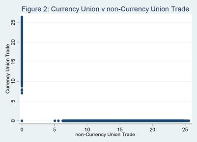
12                  THE MICHIGAN JOURNAL OF BUSINESS

     I. Introduction
              The debate as to whether a country should join a currency union was
     once cast as a struggle between competing political ideals. The left argued for
     monetary union but had little supporting evidence of possible gains. The right
     was in staunch opposition since such a step would emasculate domestic mon-
     etary policy and expose the economy to business cycle fluctuations. Recently
     a new topic of enquiry has emerged in the economic debate focusing on the
     effect monetary union has upon trade. This is the topic I address in this paper.
              Initially, monetary union was perceived to have mainly microeconom-
     ic effects through ease of price comparison and the removal of exchange rate
     transaction costs. Now authors, such as Rose (2000), have begun to explore the
     macroeconomic dimension, claiming that joining a currency union can lead
     to increases in trade of almost 400 percent.2 Others, such as Persson (2001),
     found the effect to be approximately 13 percent.3 The lack of data from well
     developed countries engaged in monetary union posed a problem for these
     investigations. However, with the introduction of the Euro as the official cur-
     rency of 11 European Union countries in 1999 and the subsequent decision of
     two more countries to join the ‘single currency’, data is becoming available
     upon which to test the currency union effect on trade for large, well developed
     countries.
              The structure of the paper is as follows. Section 2 presents a literature
     review of monetary union. I describe the contributions of some of the most im-
     portant works in the field such as Mundell (1961)4 and Rose (2000)5. Section 3
     contains a gravity model built upon optimising decisions by firms that will be
     used to estimate whether the Euro has had an effect upon trade in the member
     countries. Section 4 details the data set I use, and basic summary statistics and
     features of the data. Section 5 deals with an estimation of the currency union
     effect. A model similar to that employed by Rose (2000) is used before moving
     on to panel data estimators, dynamic panel data models and a difference-in-
     difference estimator. Further sensitivity tests are performed to analyse whether
     the inclusion of openness to trade measures affects the results and whether
     there is any evidence of trade diversion arising from the implementation of the
     Euro. Conclusions are offered in section 6.
     2
       Rose, Andrew. “One Money, One Market: Estimating The Effect of Common
         Currencies on Trade.” Economic Policy 15.30 (2000): 7-45.
     3
       Persson, Torsten. “Currency Union and Trade: How Large is the Treatment Effect?”
         Economic Policy 33 (2001): 433-448.
     4
       Mundell, Robert. “A Theory of Optimal Currency Areas.” American Economic
         Review 51 (1961): 509-517.
     5
       Rose, Andrew, Ibid.
Has the Euro Increased Trade? 13
II. Literature Review
2.1 Background
It is important to stress that the introduction of the Euro constitutes
the third stage of the Economic and Monetary Union (EMU) of the European
Union. During the first stage (1990-93), countries agreed upon the complete
abolishment of capital controls amongst European Economic Community
members. Economic convergence criteria relating to inflation rates, public
finances, interest rates and exchange rate stability were also negotiated. The
second stage of EMU (1994-1998) witnessed the signing of the Stability and
Growth Pact (SGP). This was designed to enforce fiscal discipline by pro-
hibiting member countries from running annual budget deficits in excess of
3 percent of GDP. The European Central Bank (ECB) was also established
during this epoch. It now has responsibility for setting interest rates for the
Eurozone.
The convergence criteria outline rules that future Euro members must
fulfil if they are to adopt the single currency, which constitutes the third stage.
These include the following. A country’s inflation rate must be no more than
1.5 percent higher than that of the three euro zone countries with the lowest
rates of inflation. The long-term nominal interest rate must not be more than
two percentage points higher than in the three lowest inflation member states.
The ratio of gross government debt to GDP must not exceed 60 percent at the
end of the year preceding accession. Finally, countries must have joined the
Exchange Rate Mechanism (ERM II) for two consecutive years and must not
have devalued their currency during this period. One should also note that
while Euro members coordinate monetary policy, they also cooperate on some
other economic policies. For example, tariffs are set for the EU as a whole.
2.2 The Optimal Currency Area
The origins of the optimal currency area (OCA) theory may be traced
to Mundell (1961).6 An OCA may be deemed to be a region where, in the pres-
ence of a perfectly effective monetary policy, asymmetric real shocks would
be handled in such a way that full employment and zero inflation would ensue.
Consequently the nation state may not represent an OCA. Rather an OCA may
comprise:
1. A country
2. A region, or regions, within a country
3. Regions within separate countries
6
Mundell, Robert. “A Theory of Optimal Currency Areas.” American Economic
Review 51 (1961): 509-517.14 THE MICHIGAN JOURNAL OF BUSINESS
4. Multiple countries
Mundell (1961)7 goes on to demonstrate that a country which does not consti-
tute an OCA will react sub-optimally to a negative real shock.
The following example helps to illustrate this. Imagine that two coun-
tries are identical in every respect, that they share a border, that the east of
each country produces paper and that the west produces aeroplanes. A nega-
tive shock to the demand for paper will result in higher unemployment in the
eastern regions of both countries. To counter this, the central bank could relax
monetary policy in order to restore full employment in the paper industry. In
so doing, inflationary pressures would be created in the west. Thus there exists
a trade-off between lower unemployment in one region and higher inflation in
the other. This is clearly sub-optimal. If the regions of each country were to
adopt their own currency, a Pareto improvement would follow as each region
could optimally respond to an asymmetric shock. However, this is not the first-
best solution and could be improved upon because this arrangement involves
more transaction costs due to there being four currencies. If the eastern and
western regions of each country were to join in monetary union, the costs of
international trade would be minimised and shocks to the terms of trade could
be dealt with in such a way that full employment would not come at the price
of higher inflation.
From this it is eminently clear that a key consideration when deciding
whether or not to join a currency union is the extent to which the business
cycles of the regions overlap. The greater the degree of synchronisation, the
greater will be the effectiveness of monetary policy in the enlarged region.
This will be more likely when more intra-industry trade takes place as opposed
to inter-industry trade. Under the former, industries in the regions are broadly
similar; for example, they are predominantly engaged in the production of
paper. Hence when real shocks hit the economy, monetary policy can respond
in the appropriate, counter-cyclical manner. Where trade takes place on an
inter-industry basis, real shocks are less likely to be off-set according to the
first-best solution, as the trade-off between inflation and unemployment again
exists.
The extent of integration is, thus, a key consideration when deciding
upon joining a currency union. This, however, may be endogenous as sharing
a currency could lead to greater levels of trade and thus greater integration.
Despite this, the decision to join a currency union could then be seen as the
extent to which the business cycles of different countries are synchronised.
Foregoing the national currency entails a loss of monetary autonomy thus
7
Mundell, Robert. “A Theory of Optimal Currency Areas.” American Economic
Review 51 (1961): 509-517.Has the Euro Increased Trade? 15
preventing a policy-maker from dampening business cycle fluctuations. The
degree of synchronisation between a group of countries will then depend upon
the nature of trade between them.8 Theoretically, pan-national business cycles
could either become more or less integrated. If countries were to become more
specialised in the areas in which they hold a comparative advantage, closer
trading relations would lead to more idiosyncratic business cycle patterns.
Consider, for example, a two country scenario where country A is relatively
more efficient in producing apples while country B holds an advantage in the
production of bananas. Post trade liberalisation, each country could specialise
in the production of the good they produce most efficiently and then trade
apples for bananas. The effect of trade then increases the degree of industrial
specialisation. Business cycles would become more idiosyncratic since each
country is buffeted by different real shocks.
However, several authors have found that the greater the extent of in-
tegration, the more trade will increase, leading to more highly correlated busi-
ness cycles between the countries involved. Frankel and Rose cite Eichengreen
(1992),9 Kenen (1969),10 and Krugman (1993)11 as having all noted this feature
of closer integration. Frankel and Rose use instrumental variables to estimate
empirically whether trade intensity results in greater income correlation. The
regression they use is of the following form:
Corr (v, s )i , j ,τ = α + βTrade (w)i , j ,τ + ε i , j ,τ (1)
The motivation for using instruments is twofold. Firstly, the error component
is likely to be correlated with the trade variable in either the time or spatial di-
mension. For example, the Spanish-Portuguese trade observation for December
may not be independent of that for November, or independent of the French-
Spanish observation. Secondly, ordinary least squares (OLS) is inappropriate
as countries are more likely to peg their currency to that of their main trading
partners in order to eliminate exchange rate instability more effectively; that is,
members join in a non-random manner. The instruments used are the natural
logarithm of distance between business hubs, a dummy variable for geographic
adjacency and a dummy variable that indicates a common language. Frankel
8
Frankel, Jeffrey, and Andrew Rose. “The Endogeneity of the Optimum Currency
Area Criteria.” Economic Journal 108 (1998): 1009-1025.
9
Eichengreen, Barry. “Should the Maastricht Treaty be Saved?” In Frankel, Jeffrey,
and Andrew Rose. Economic Journal 108 (1998): 1009-1025.
10
Kenen, Peter. “The Theory of Optimum Currency Areas: an Eclectic View.” In
Frankel, Jeffrey and Andrew Rose. Economic Journal 108 (1998): 1009-1025.
11
Krugman, Paul. “Lessons of Massachusetts for EMU.” In Frankel, Jeffrey and
Andrew Rose. Economic Journal 108 (1998): 1009-1025.16 THE MICHIGAN JOURNAL OF BUSINESS
and Rose found that, regardless of whether they normalised by trade or GDP,
greater intensity of international trade led to higher correlations between in-
come. This effect was strongly positive and statistically significant.
Another channel through which adjustment may occur in response to
a real shock is labour mobility. If labour is sufficiently mobile, it could move
from an area stuck in recession to one where job opportunities exist. This
would help dampen business cycles and is often mooted as the reason why
the United States constitutes an OCA while the European Union does not. The
language barrier, which exists between the European nations, is not present in
the United States. Despite this, labour mobility in the US is not of a sufficient
magnitude to dampen business cycle fluctuations at regional level.
2.3 Reasons for Adopting/Maintaining a National Currency
The post-World War II era has seen the number of countries more than
double, accompanied by an unprecedented increase in economic integration
and interdependence. It is somewhat surprising, therefore, that the number of
national currencies in circulation through out the world has increased dramati-
cally since the greater the level of integration the greater the level of synchro-
nisation. This reduces the opportunity cost of removing a currency. However,
greater economic integration would imply that the costs of a national currency
would be higher arising from exchange rate transaction costs. One would have
to believe that the national unit is chosen to correspond with the OCA. This
would seem to be incidental. It is possible that the growth in the number of
countries has resulted in interregional trade being relabelled as international
trade and that this process has allowed independent monetary policy to be used
to stabilise the (smaller) economy. Alesina et al (2000) refute this idea.12
Numerous authors have suggested that pride and sovereignty are the
principle motives for maintaining a national currency. However, citizens do
not appear to mind when the national currency is renamed following an infla-
tionary crisis. In fact one would have thought that national sports teams inspire
greater devotion and euphoria than does a currency. Inflation aversion could be
a disguise for national pride. Decimalisation and the introduction of the Euro
were associated with increases in prices. This theoretically could have been
caused by menu-cost effects. According to the Barro-Gordon model of mon-
etary policy, agents may prefer decisions to be made nationally because the
preferences of the policy maker are more representative of attitudes towards
inflation. This could be the reason for some countries’ citizens being so op-
12
Alesina, Alberto, Robert Barro, and Silvana Tenreyro. “Optimal Currency Areas.”
NBER Working Paper Series Working Paper 9072 (2002).Has the Euro Increased Trade? 17
posed to the adoption of a foreign currency as the new policy maker may have
a different attitude towards the trade-off between inflation and output.
Irrespective of the number of currencies in circulation, Mundell (1961)
noted that the use of multiple currencies results in a deadweight loss because
of the higher transaction costs agents must bear when they engage in interna-
tional trade13. Mundell then goes on to state that while the optimal number of
currencies is not infinite, although this would mitigate a ‘perfect’ response to a
real shock, the transactions costs arising from trade would be overwhelming.
Equally the optimal number would not be one as this could be welfare decreas-
ing due to the inability to stabilise the domestic economy.
2.4 Public Goods, Inflation and Monetary Union
Small countries may not be big enough to provide public goods ef-
ficiently as they cannot exploit economies of scale in the way that larger
countries can.14 Two areas that illustrate this idea are military defence and
national currency. With both, the expense of ‘going it alone’ is high due to the
fixed costs involved. Small countries have overcome the problem of military
defence by forming alliances. The decision of the Baltic states to join NATO
is an example. Regarding currency, countries that have seceded from others
have been notably reluctant to adopt the currency of a large trading partner.
Montenegro and East Timor are recent exceptions. This, presumably, is be-
cause the only viable currency of the newly independent country would be that
of the nation from which it has just seceded. In this case, nationalist sentiment
or revulsion for the former occupier may preclude monetary union.
A second, more powerful argument for monetary union than the public
goods case is the conduct of monetary policy. Let us suppose that there exists
a country that is particularly prone to expansionary monetary policy. An infla-
tion bias as demonstrated by Barro and Gordon (1983)15 may exist. This bias
could be eliminated or reduced by pegging the national currency to that of a
country with monetary discipline and an aversion to inflation. The monetary
policy of the inflation-prone country would then effectively be determined by
the disciplined central bank. This would eliminate the tendency to follow a
persistently expansive, monetary policy and, consequently, the inflation bias.
13
Mundell, Robert. “A Theory of Optimal Currency Areas.” American Economic
Review 51 (1961): 509-517.
14
Alesina, Alberto, Enrico Spolaore, and Romain Wacziarg. “Trade, Growth, and
the Size of Countries.” Harvard Institute of Economic Research Working Papers
Working Paper 1995 (2002).
15
Barro, Robert, and David Gordon. “A Positive Theory of Monetary Policy in a
Natural Rate Model.” Journal of Political Economy 91 (1983): 589-610.18 THE MICHIGAN JOURNAL OF BUSINESS
One could argue that short run considerations, such as recessions, pro-
vide support for maintaining monetary autonomy. Policy makers could then
(theoretically) end a recession. A classic example of this was the UK’s exit
from ERM in 1992 (although one could argue currency speculation was a ma-
jor factor). It could be further argued that a country with a preference towards
expansionary monetary policy would never want to forego monetary autonomy
as it could always raise welfare by increasing output beyond its natural rate.
While this is feasible in the short run, such a policy is unsustainable over a
longer horizon. Agents would rationally expect consistent monetary expansion
and respond by raising their inflation expectations. Prices would persistently
increase with no offsetting gains in output. The gains to eliminating the infla-
tion bias would then be large.
One means of eliminating an inflation bias might be through the use
of fixed exchange rates. These, however, tend to create imbalances in finan-
cial markets. The currency crises of the 1990s demonstrated that developed
countries were just as susceptible to attack as developing nations. Numerous
authors have noted that, when the costs of maintaining the fixed exchange rate
were too high or where the domestic economy could benefit through the use
of domestic monetary policy, a speculative attack would force an end to a peg.
Hence fixed exchange rates lack full credibility. Over the past 40 years, they
have not been fixed irrevocably,16 and many have been eliminated, which may
provide the stimulus for a speculative attack.
A currency union represents a more durable commitment that delivers
the same outcome. The costs of abandoning the new currency are very high. In
this situation, the domestic inflation rate is as in 2.
π i = π j + Δρ (2)
Inflation in country i is composed of the inflation rate in the anchor country,
j, plus or minus the change in relative price level between the domestic and
anchor economy.17 As noted previously, the higher the correlation between
business cycle shocks, the greater the capacity for monetary policy to be used
in a counter-cyclical manner to achieve stabilisation.
2.5 Trade Benefits
The public goods and inflation arguments for joining a currency
16
Alesina, Alberto, Robert Barro, and Silvana Tenreyro. “Optimal Currency Areas.”
NBER Working Paper Series Working Paper 9072 (2002).
17
Alesina, Alberto, Ibid.Has the Euro Increased Trade? 19
union are attractive. However, the empirical literature that began to
emerge during the mid-1990s suggests that perhaps the most important conse-
quence of common currency areas was the increase in trade.
One of the first publications in this area was McCallum (1995).18 This
paper examined whether the US-Canadian border had had a substantial effect
upon trade between states and provinces using 1988 import and export data on
the 10 Canadian provinces and the 30 US states that accounted for more than
90 percent of Canada-US trade. To estimate this, a simple gravity model was
used,
xij = a + byi + cy j + dDIST ij + eDUMMY ij + uij (3)
where xij is the logarithm of trade between region i to region j, yi and yj are the
logarithms of GDP in region i and j respectively, DISTij is the logarithm of the
distance between i and j, DUMMYij is a dummy variable equal to 1 for state-to-
province trade and equal to zero otherwise, and uij is an error term.
McCallum’s headline-grabbing finding was that province-to-province
and state-to-state trade was 22 times greater than province-to-state trade. This
was even more remarkable as, at that time, the US-Canadian border was seen
as being one of the most open in the world since a free trade agreement had
been signed in 1988. In addition, both countries used the same language and
had solid laws governing the enforcement of contracts. One of the reasons
advanced as a possible explanation for such a large difference in trade volumes
was the use of different currencies.
However, the findings of McCallum were not as robust as first thought
due to omitted variable bias and the failure to take into account the small
size of the Canadian economy. The simple specification of equation 2 fails
to acknowledge multilateral resistances as well as bilateral resistances. The
bilateral barriers to trade between countries are manifested through tariffs,
non-tariff barriers and the currencies used, to list just a few of the impediments
to trade. Anderson (1979) defines multilateral resistance as the resistances to
trade arising between country i and all other countries except j. 19 Multilateral
resistances to trade affect the trade between country i and j because the resis-
tances to trade between i and all countries other than j will indirectly determine
how much i trades with j. For example, if a given country, k, has lower trade
barriers with i than the average barrier between i and j, firms in i can deal more
18
McCallum, John. “National Borders Matter: Canada-U.S. Regional Trade
Patterns.” American Economic Review 85 (1995): 615-623.
19
Anderson, James. “A Theoretical Foundation for the Gravity Equation.” American
Economic Review 69 (1979): 106-116.20 THE MICHIGAN JOURNAL OF BUSINESS
cheaply with firms from k than from j, making them more likely to trade with
k. In summary, after controlling for size, interregional trade is a decreasing
function of the bilateral trade barrier between i and j, relative to the average
barrier to trade of i and j with all other regions. Anderson and van Wincoop
(2003) cite multilateral resistances as being the omitted variables which drive
McCallum’s results.20
The second factor leading to bias in the estimates was the failure to
account for the small, open nature of the Canadian economy. Small econo-
mies tend to engage in trade to a much greater extent than large ones because
their domestic markets tend to be constrained by their small population.
Consequently, a small economy must engage in international trade if it is to
buy and sell goods and services. Anecdotal evidence exists to support this. For
example, Ireland and Belgium, which are both small and open economies, ex-
hibit openness to trade ratios well in excess of 100 percent. This means that the
ratio of trade to GDP is greater than 1. It was, therefore, almost inevitable that
the Canadian economy would be more susceptible to barriers to trade because,
unlike the United States, a much greater percentage of its trade was conducted
outside the country rather than inside. A small barrier between Canada and
the rest of the world has large effects on the multilateral resistances to trade
as the economy is more exposed to international trade. However, the effect of
the border on the US is much smaller because a large percentage of its trade is
conducted between its own states. This explains why the border affects it to a
lesser degree.
In an attempt to ascertain the accuracy of McCallum’s findings,
Anderson and Van Wincoop (2001) first derived a theoretical gravity model
based on constant elasticity of substitution (CES) preferences21 In so doing
and controlling for size and distance, they incorporated multilateral resistance
terms. Using 1993 data they estimated that the Canadian-US border reduced
trade between the countries by 44 percent. They also found that the border re-
duced trade with other industrialised nations by 30 percent. The within-country
increase in trade after imposing the border was also much lower; a 6- fold
increase and a 25 percent increase for Canada and the US respectively.
2.6 Trade and Currency Unions
The period prior to the introduction of the Euro saw numerous publi-
cations attempting to quantify the possible effect of monetary union on trade.
In a seminal paper in this area, Rose (2000) used data drawn from existing cur-
20
Anderson, James, and Eric Van Wincoop. “Gravity with Gravitas: A Solution to the
Border Puzzle.” Boston College Working Papers Working Paper 485 (2000).
21
Ibid.Has the Euro Increased Trade? 21
rency union members.22 It was found that currency unions raised trade between
members by approximately 400 percent using an OLS estimator. Further pa-
pers by Rose established that the effect was robust and statistically significant
to various model specifications.
Rose and van Wincoop (2001) espoused the view that currency unions
had such an impact because of the efficiency gains associated with using one,
rather than multiple, currencies.23 This was puzzling since the cost of hedging
was low due to the prevailing, extensive derivative markets. The authors then
hypothesised that a shared currency could lead to a deepening of trading rela-
tions and increased price transparency across countries. This could prove to
be trade enhancing. The central weakness of this finding was, however, that it
was based on a very small sample of observations drawn from countries which
were either small, poor or remote or, in some instances, all three. Several were
also island nations and therefore, more likely to engage in trade. Hence the
conclusions of this paper, while seemingly robust and highly significant, could
not automatically be applied to the large, developed nations that were about
to introduce the Euro as their currency. The currency unions used by Rose
(2000)24 tended to comprise nations that were geographically disparate and
usually had within them one large developed country and a number of small
and/or poor nations or colonies. France and Reunion is a typical example.
Quah (2000) remarked that of the 33903 bilateral trade observations, a mere
320 were between currency union members.25 This meant that the results were
drawn from a sub-sample which constituted less than 1 percent of the total
observations.
An ambitious attempt to resolve the ‘true’ effect of currency unions
on trade entailed the use of a non-parametric matching technique by Persson
(2001).26 This was prompted by the small number of changes in the monetary
regime of most countries. The currency union effect could, therefore, only be
gauged through cross-sectional variation rather than through observation of
22
Rose, Andrew. “One Money, One Market: Estimating The Effect of Common
Currencies on Trade.” Economic Policy 15.30 (2000): 7-45.
23
Rose, Andrew, and Eric Van Wincoop. “National Money as a Barrier to
International Trade: The Real Case for Currency Union.” American Economic
Review 91.2 (2001): 386-390.
24
Rose, Andrew. “One Money, One Market: Estimating The Effect of Common
Currencies on Trade.” Economic Policy 15.30 (2000): 7-45.
25
Quah, Danny. “One Money, One Market: Estimating The Effect of Common
Currencies on Trade.” In Rose, Andrew. Economic Policy 15.30 (2000): 7-45.
26
Persson, Torsten. “Currency Union and Trade: How Large is the Treatment Effect?”
Economic Policy 33 (2001): 433-448.22 THE MICHIGAN JOURNAL OF BUSINESS
the difference before and after monetary union. Persson also argued that if the
currency union variable was correlated with any of the other regressors, or if
selection into a currency was non-random, then the linear regression frame-
work used in Rose might have produced biased results.
Using this methodology, Persson was able to construct a treated group
(members of a currency union) and a control group (non-members) which were
comparable in that they had the same regressors. The results were then gener-
ated using non-parametric estimators which yielded a treatment effect ranging
between a 15 and 63 percent increase in trade. The standard errors, however,
were of a magnitude that rendered the results statistically insignificant.
III. The Gravity Model
In this section I outline the gravity model I will use to estimate the
currency union effect of the Euro. The empirical literature has tended to re-
main silent regarding the theoretical foundations of such models. This may be
partly explained by how well the models work empirically despite their lack of
microeconomic foundations. The theoretical literature reveals a great deal of
variety as to how these models were derived. For example, Anderson’s (1979)
model is constructed using goods distinguished by their region of origin.27
Bergstrand (1989) derives the gravity equation from an economies of scale
trade model.28 Deardorff (1995) demonstrates that a Heckscher-Ohlin model
may be used as a premise for deriving a gravity equation.29 One unifying ele-
ment among all these papers is the use of CES preferences.
3.1 The Model
Traditionally, it has been the case that empiricists have used gravity
models to estimate the effect of monetary union on trade. An example of this
model is:
ln T ij = β1 ln Yi + β 2 ln Y j + β 3 DIST ij + β 4 ln S i + β 5 ln S j + β 6 X ij + β 7 cui + ε ij (4)
where Tij represents trade between i and j, Yi and Yj stand for GDP in i and j,
respectively, DISTij is the distance between the regions, Si and Sj are measures
of the size of i and j, usually taken as meaning either population or land mass,
27
Anderson, James. “A Theoretical Foundation for the Gravity Equation.” American
Economic Review 69 (1979): 106-116.
28
Bergstrand, Jeffrey. “The Gravity Equation in International Trade: Some
Microeconomic Foundations and Empirical Evidence.” Review of Economics
and Statistics 67 (1985): 474-481.
29
Deardorff, Alan. “Determinants of Bilateral Trade: Does Gravity work in a
Neoclassical World?” NBER Working Paper Series Working Paper 5377 (1983).Has the Euro Increased Trade? 23
Xij is a matrix that contains a number of other possible determinants of trade
such as a free trade dummy variable, a common language dummy variable
and a dummy variable indicating a shared colonial history, and so on, cuij is a
dummy variable equal to one if the countries share the same currency and ε ij is
a well behaved error term.
3.2 Features of the Model
The main ideas behind the model are that countries with a high GDP
will trade more because they have/demand a greater number of goods, while
distant countries are assumed to trade less because the greater the distance,
the greater the costs regarding transportation and creation of trading contacts
and relationships. However, while the models work well empirically with
R-squared values of approximately 0.80 reported in Bergstrand (1985)30 for
the years 1965, 1966, 1975 and 1976, the theoretical foundations underpinning
them tend to be simplistic and based upon intuitive arguments rather than on
microeconomic fundamentals.
Owing to the lack of a single unifying framework, omitted variable
bias and model uncertainty arise. As noted previously, omitted variables in
the shape of multilateral resistance terms, was one of the principle reasons
why McCallum (1995) found the Canada-US border to have had such a large
impact on trade between the countries.31 Similarly, authors often include a bat-
tery of dummy variables to control for determinants of trade such as free trade,
colonial heritage and language.
IV. Data and Methodology
4.1 Data Sources and Definitions
This paper uses a large panel data set, constructed from a variety
of sources, resulting in 51,831 observations drawn from 12 Eurozone and
3 non-Eurozone countries’ trade with 187 countries. A complete list of the
trade partner countries in the data set is provided in Table 10 in Appendix 1.1.
The Eurozone members in the sample are Austria, Belgium, Finland, France,
Germany, Greece, Ireland, Italy, Luxembourg, the Netherlands, Portugal and
Spain, while the non-Eurozone members are Denmark, Sweden and the United
Kingdom. All of these countries adopted the Euro in 1999 with the exception
30
Bergstrand, Jeffrey. “The Gravity Equation in International Trade: Some
Microeconomic Foundations and Empirical Evidence.” Review of Economics
and Statistics 67 (1985): 474-481.
31
McCallum, John. “National Borders Matter: Canada-U.S. Regional Trade
Patterns.” American Economic Review 85 (1995): 615-623.24 THE MICHIGAN JOURNAL OF BUSINESS
of Greece, which joined in 2001. Other currency unions present in the data set
are between France and French Guiana through the use of the French franc
and between Belgium and Luxembourg through a fixed exchange rate. For
each of these currency unions, the member countries are engaged in monetary
union for the entire period covered by the sample. As with several of France’s
overseas Departments, French Guiana adopted the Euro as its official currency
at the same time as France. Similarly, Belgium and Luxembourg also adopted
the Euro as their official currency in 1999.
For the period 1980-2004, the real GDP per capita data are constructed
using Penn World Tables 6.2 edition. Real GDP per capita is expressed in
thousands of US dollars with 2000 prices acting as the base year. For the same
period, the population data is also constructed using the Penn World Tables
6.2 edition data. The distance between countries is based on the great circle
distance between the two countries, with the central point in each country be-
ing its capital city.
Data on bilateral trade between countries comes from the United
Nations Statistics Division’s Common Database. As is usual in this literature,
bilateral trade is taken to be the sum of imports and exports during a given
year. One point to be noted in the dataset is that the value of exports from
country i to country j is not necessarily the same as the value of imports into j
from i for any given observation, that is
x ij ≠ mij
To overcome this measurement error problem, I take a simple mean of the trade
statistics for each country. However, since there is a danger that the differences
between the reported trade statistics could be large, I will also use a weighted
least squares (WLS) estimator.
The common language dummy variable is assigned a value of 1 when
country i shares the same language as j and 0 otherwise. This information is
taken from the CIA World Factbook. A common language is assumed when
one of the official languages of country i is the same as that used in country j.
Consequently, a country may share a common language with more than one
trading partner despite its trading partners using a different language. A good
example of this is Belgium which has three official languages.
The free trade dummy is equal to one if a country is a member of the
European Free Trade Association (EFTA), the European Union or the European
Economic Community. Otherwise, it is equal to zero. For simplicity, I assume
that a free trade agreement (FTA) is in place if two countries have signed a
bilateral trade agreement. The shared colonial history dummy takes a value of
1 if the trading partners were engaged in a colonial relationship at any point inHas the Euro Increased Trade? 25
the post-1945 period. Otherwise it assumes a value of zero.
Finally, the currency union dummy takes a value of 1 from the year
that a country adopts the Euro as its national currency or the currency of an-
other country. Otherwise the variable assumes a value of zero. Despite the in-
troduction of the Euro in physical form in 2001, all Eurozone members, except
Greece, are taken to be engaged in monetary union from 1999 since this was
the year in which all national currencies were unilaterally fixed at their agreed
exchange rate. This, in effect, made the Euro each member’s national currency
and the ECB responsible for monetary policy throughout the bloc.
4.2 Description of the Data
With the data collected, I have assembled a large unbalanced panel
data set. The unbalanced panels are caused, in some cases, by poor records and
misreporting of the actual data, which might lead to measurement error and
thus biased results. Secession has also meant that many countries have entered
the panel over the period while the unification of a few countries has led to
some dropping out. The Soviet Union and other command-based communist
countries are excluded because they bear little resemblance to the market
economies with which I am concerned.
Belgian statistics are only reported for 1998 to 2004 and Luxembourgian
statistics for 1999-2004. Prior to 1998, all data for the two countries are re-
ported as though they were one country, an artefact of their economic and
monetary union agreement that has been in place since 1921. A consequence
was that trade statistics were produced for Belgium-Luxembourg rather than
for each country. Data are available for the separate entities post-1998 as a
result of a ruling by the EU which demanded that individual countries report
trade and GDP on a country specific basis.
There is a danger that the inclusion of Luxembourg could bias
the results of the estimation procedure. This is caused by the small size of
Luxembourg in both the geographical and economic sense and also by its very
high GDP and openness to trade. To establish whether Luxembourg should be
omitted from the sample, I perform a series of robustness checks.
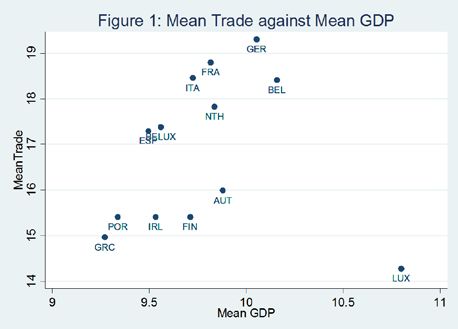
From Figure 1, it is clear that Luxembourg’s very high GDP and low
relative level of trade could potentially bias the results downwards or even
impose a negative relationship upon any linear regression. To verify whether
this is the case, I perform robustness checks to see whether the inclusion of
Luxembourg seriously affects the regression estimates. This is achieved using
a pooled OLS regression on the entire period.
I find that the inclusion of Luxembourg does have an influence on the26 THE MICHIGAN JOURNAL OF BUSINESS
results. However, this is not to the extent that the coefficients depart hugely
from the results derived when only the other 11 countries are included. Indeed
none of the variables change in sign when Luxembourg is included and the
largest change in the estimated results is a meagre 0.05 reduction in the GDP
per capita coefficient. With this said, I turn my attention to summary statistics
and correlations amongst the variables prior to embarking upon any regression
analysis. The correlations between each of the variables are shown in Table 1
below.
It is clear from this that trade is strongly correlated with many of the
variables since five of them have correlation values in excess of 0.20. There
also appears to be a modest relationship between the currency union dummy
variable and trade with a correlation of approximately 0.20. Indeed, currency
unions in the sample seem to exhibit correlations with most of the variables,
with the exception of language and colonial history. This is unsurprising since
the sample covers the Eurozone countries which have bilateral trade agree-
ments through their membership of the European Union and tend to be fairly
rich, geographically close.
4.3 Estimation Procedure
The gravity equation from the previous section serves as the basis of
the estimation procedure that will be used to quantify the effect of the EuroHas the Euro Increased Trade? 27
upon its members’ trade. However, I shall append the model with the dummy
variables detailed above. This is similar to the approach implemented by Rose
and van Wincoop (2001).32 It would be unwise to assume that the sole deter-
minants of bilateral trade flows are GDP, prices and distance given the extent
to which some of the variables are correlated with trade demonstrated in Table
1. For example, free trade agreements, colonial histories, a shared language,
a shared border and the same currency all affect whether countries engage in
trade through the removal of tariff boundaries and the establishment of rela-
tions between individuals and firms, and so on.
Table 1: Correlations
Variable Trade GDPiGDPj GDPiGDPj per capita Distance Border
Trade 1.00
GDPiGDPj .8137 1.00
GDPiGDPj per capita .4871 .4724 1.00
Distance -.4440 -.2467 -.2515 1.00
Border .2467 1.564 .1613 -.3866 1.00
Language .0010 -.0924 -.0518 .0592 .0732
FTA .3362 .2410 .3630 -.3900 .2472
Colonial History .0636 -.0162 -.1117 .0015 -.0202
Currency Union .2023 .1677 .2284 -.2144 .1708
Language FTA Colonial History Currency Union
Language 1.00
FTA -.0336 1.00
Colonial History .3275 -.0355 1.00
Currency Union .0010 .5212 -.0190 1.00
V. Empirical Analysis
I shall now consider empirical testing of the currency union effect
upon trade using the gravity equation to quantify the effects of the Euro upon
trade in the 1999-2004 period.
5.1 Difference-in-Difference Estimation
A simple means of estimating the effect of the Euro upon trade would
be to analyse how trade responded in the cases where a country did and did
not join the single currency. However, one of the main difficulties in resolving
the currency union effect upon trade is that we do not know what the level of
trade would have been had a specific country not engaged in monetary union.
In a laboratory experiment, this could be accomplished through administering
treatment to one specimen (the treated group) while holding conditions con-
32
Rose, Andrew, and Eric Van Wincoop. “National Money as a Barrier to
International Trade: The Real Case for Currency Union.” American Economic
Review 91.2 (2001): 386-390.28 THE MICHIGAN JOURNAL OF BUSINESS
stant in all regards for an identical specimen that does not receive the treatment
(the control group). This provides a natural experiment since conditions are
the same in every way for both the treated and the control group. One could
then gauge whether the treatment had an effect and quantify its magnitude.
Ideally, one could use a similar procedure to ascertain the currency
union effect on trade. However, finding a control group for the experiment is
difficult. There are inherent differences in government policy, culture and the
model of capitalism between the countries which adopted the Euro as their
currency and the rest of the world. Despite this, there are a number of countries
that could be considered for use in a control group. One possible control group
could be the non-Eurozone OECD countries. There are many similarities
between these well developed, rich countries which have similar institutions
to those nations using the Euro. Most OECD members also have free trade
agreements in place and similar GDP (although mainly through multilateral
rather than bilateral agreements). Although there are similarities, there are also
reasons to believe that the OECD would not constitute a good control group.
Many of these, such as Japan and Mexico, are geographically distant, not just
from the EU but from one another. Secondly, OECD countries do not tend to be
integrated to the same extent politically or economically as is the Eurozone.
However, the decision of Denmark, Sweden and the United Kingdom
to remain outside the Euro presents a potential control group which has much
in common with the Eurozone countries.33 They are EU members and thus
share in the political and economic agreements of the supranational organisa-
tion. They are geographically close and conduct a large amount of trade with
Euro members (for example, the UK conducts approximately 60% of its trade
with Eurozone countries). One could also argue for the inclusion of some of
the Eastern European countries such as the Czech Republic and Poland, but
these are excluded since they only became EU members in 2004.
The object of difference-in-difference (DD) estimation is to uncover
the effects of a change in policy, in this case the effect of the Euro upon trade.
DD estimates are found by applying an OLS estimator to the cross-sectional
panel data in the data set for the years prior to the change and then to the post-
treatment period for both the treated and control groups. First, I compute aver-
age trade for each treated and control country for the pre-1999 and 1999-2004
periods. Baier et al. (2002) recommend using aggregation of the data in the
before-and after-treatment periods in order to overcome problems of serial
33
A possible downside to including Denmark is that the Krone was pegged to the
Euro over the period under inspection.Has the Euro Increased Trade? 29
correlation which often afflict DD estimators.34 The direction of the bias in the
standard errors that serially correlated observations will have depends upon
whether there is positive or negative serial correlation. Positive serial correla-
tion will result in under-reported standard errors while the opposite will occur
if negative serial correlation is present.
To obtain the DD estimator I generate three dummy variables. The
first is called post, which is equal to one if the observation comes from the
post-1999 period. The second dummy is treatment, which is equal to one if the
observation comes from the group that engaged in monetary union. Finally, I
generate an interaction term, post*treatment, which is the result of multiplying
post and treatment together. This is the coefficient of interest because it shows
the estimated effects of changing the currency to the Euro. It is then possible
to estimate the following equation to obtain the treatment effect:
T i = β 1 posti + β 2 treatmenti + β 3 post* treatmenti + ν i (5)
The DD estimate is then βˆ 3 . The results of this regression are given in Table
2.
Table 2: Difference-in-Difference Estimates
Dependent Variable: Bilateral Trade
post -.006
(.06)
treatment -1.36
(.06)
post*treatment .78
(.07)
2
R .0194
Number of observations 51831
Robust standard errors in parentheses
The results indicate that trade decreased for the control group between
the two periods by 0.006 percent but this is both economically and statistically
insignificant. The coefficient on treatment shows that among the countries that
adopted the Euro, trade was initially on average less than among the control
group, but this increased markedly in the post-1999 period as demonstrated by
the post*treatment coefficient. Indeed, the treatment effect of the Euro is found
to be colossal, with a coefficient of 0.78. The estimate is also highly significant
34
Baier, Scott, Jeffrey Bergstrand, and Peter Egger. “The New Regionalism: Causes
and Consequences.” Économie Internationale 109 (2007): 9-29.30 THE MICHIGAN JOURNAL OF BUSINESS
with a t-statistic greater than 11. This would appear to suggest that the cur-
rency union effect on trade is large regardless of whether countries are small,
poor and remote or large, well developed and geographically centric. However,
the results in Table 2 should be treated with caution. Regardless of whatever
concerns one may have about the practical uses of the R2 in applied economics,
a value of .0194 is hardly robust. Indeed, this casts doubt upon whether the
estimates are correct given that, at best, they explain a mere 2 percent of the
variation in the dependent variable, trade. This leads me to question whether
the results are in fact a product of a statistical rather than an economic relation-
ship.
It is important to note that the DD estimates fail to take into account
the endogeneity of the treatment effect. This could lead to biased estimates
since the assignment of countries into the treatment and control groups is non-
random. If the results were to be unbiased, then firms and agents in the period
prior to 1999 must be unaware that the treatment will occur. However, this is
unlikely to be the case as the Maastricht Treaty, signed in 1993, would have
signalled that countries were preparing to engage in future monetary union.
Firms and individuals could then have responded by taking decisions to pre-
pare for this eventuality.
5.2 OLS Regressions
The model to be estimated takes the following form:
⎛ MiM j ⎞
xit = β 0 M i M j + β 1 ⎜ ⎟ + β 2 DIST ij + β 3 Borderij + β 4 Lang ij + β 5 FTA ij
⎜ Pop Pop ⎟
⎝ i j ⎠ (6)
+ β 6 Colony ij + φcu ij + ε ij
where Mi and Mj are log GDP for country i and j, respectively, Popi and Popj
are log population for i and j, respectively, DISTij is the log distance between
i and j, Borderij is a dummy variable equal to one if i and j share a common
border, FTAij represents whether the trading partners have a bilateral free trade
agreement, Colonyij indicates whether i and j have a shared colonial history
post-1945, and cuij is a dummy variable equal to one if the countries use the
Euro as their official currency.
Rose (2000) used pooled data from the years 1970, 1975, 1980, 1985
and 1990.35 He then used an OLS estimator with robust standard errors to
determine the effects of monetary union upon trade. It is important to note
that this did not incorporate clustering effects. I begin the analysis by adopting
35
Rose, Andrew. “One Money, One Market: Estimating The Effect of Common
Currencies on Trade.” Economic Policy 15.30 (2000): 7-45.Has the Euro Increased Trade? 31
an approach similar to that of Rose, although I pool the data across the entire
sample I have available. Since the estimation procedure relies upon a pooled
OLS model, I use a Breusch-Pagan test to ascertain whether the disturbance
terms are spherical. This produced an LM value of 2985.88, which is greater
than the critical value of 2.73 at the 5 percent level of significance, leading to a
rejection of the null of homoskedasticity. I then implement heteroskedasticity-
robust standard errors.
The results of the regressions for the 1980-2004, 1980-1998 and
1999-2004 periods are reported in Table 3. I also include the Rose results for
comparison. For the entire sample period, with the exception of the currency
union dummy, all the variables appear correctly signed and are statistically sig-
nificant. Some of the t-statistics are huge with values in excess of 20. However,
this is not unreasonable and the magnitudes are similar to those reported else-
where in the literature.
Table 3: OLS Regressions
Dependent Variable: Bilateral Trade
1980-2004 1980-1998 1999-2004 Rose 1970-1990
GDPiGDPj .93 .91 .96 .80
(.004) (.004) (.01) (.01)
GDPiGDPj per capita .17 .26 .30 .66
(.01) (.01) (.02) (.01)
Distance -.89 -.92 -.77 -1.09
(.02) (.03) (.03) (.02)
Border .52 .39 .45
(.05) (.06) (.08)
Language .91 .92 .81 .40
(.03) (.04) (.06) (.04)
FTA .79 .63 .68 .99
(.03) (.03) (.06) (.08)
Colonial History 1.50 1.57 1.54 2.40
(.06) (.07) (.13) (.07)
Currency Union -.38 -2.68 .11 1.21
(.04) (.10) (.04) (.14)
2
R .7432 .7402 .7857 .63
Number of observations 38498 27860 10638 22948
Robust standard errors reported in parentheses
The currency union effect is actually found to reduce trade between
members of a common currency by approximately 38 percent over the entire
period. However, this is more an artefact of the estimation procedure used and
outliers. To see this, consider Figure 2 below.32 THE MICHIGAN JOURNAL OF BUSINESS
This demonstrates that, when OLS is applied to the model, countries
which are members of currency unions are drawn from a different panel than
non-members. Consequently when the regression is run, the OLS estimator
establishes a negative relationship, as this is the nature of the distribution.
Over the 1980-1998 period the currency union coefficient is far greater
than that for the whole sample period and assumes a fairly implausible yet
statistically significant value. However, inference is based upon a mere 16
observations which include only France and a dependency, French Guiana.
Thus the estimates for this period are of little significance. The estimates for
the 1999-2004 period, when the single currency came into effect, are of greater
interest. It appears that GDP per capita is a better determinant of trade during
this period, whereas the effect of distance between trading partners, while still
significant at the 5 percent level, has decreased. A similar trend has occurred
regarding language, which might signal a greater degree of interdependence
across countries. However, the central finding of this regression is that the
introduction of the Euro has served to increase trade among the 11 members by
approximately 11 percent and the accompanying t-statistic is 2.20.
An increase in trade of 11 percent pales in comparison to the 397 per
cent gains in trade found by Rose. However, the sample I use may be a better
barometer in that it has within it countries which are not small, remote or poor.
Only one island economy is included. The value I have found could be ‘low’
because the level of trade which had previously taken place amongst Eurozone
members was high. In effect, there may be diminishing returns to trade follow-Has the Euro Increased Trade? 33
ing the introduction of a common currency. The greater the volume of trade
already conducted between members could result in the common currency
having a lesser impact because of the established trading links and the free
trade agreements covering all European Union members.
The results I have obtained for the period differ quite starkly from
those of Rose. This is hardly surprising given the different data sets that cover
different years. Ignoring this, even for the period in which the Euro is adopted,
its estimated effect on trade is small in comparison to the Rose findings (0.11
against 1.21). This may be because the countries in Rose’s data set have en-
gaged in monetary union for much longer periods of time. This means the
effect of using a different currency has had sufficient time to permit the es-
tablishment of trading relationships. However, it could also be the differences
in the results are caused by the different countries used in mine and Rose’s
datasets. Perhaps the trade benefits for large countries are small.
Table 4: WLS Regressions
Dependent Variable: Bilateral Trade
1980-2004 1980-1998 1999-2004
GDPiGDPj .86 .86 .91
(.006) (.006) (.005)
GDPiGDPj per capita .23 .26 .40
(.01) (.01) (.01)
Distance -.85 -.88 -.73
(.02) (.03) (.04)
Border .56 .48 .48
(.01) (.02) (.02)
Language .73 .78 .59
(.01) (.01) (.02)
FTA .69 .69 .53
(.01) (.01) (.02)
Colonial History 1.49 1.53 1.54
(.02) (.02) (.03)
Currency Union -.31 -2.49 .16
(.02) (.09) (.02)
2
R .7569 .7544 .7857
Number of observations 38498 27860 10638
Robust standard errors reported in parentheses
In Table 4 are the results from a weighted least squares (WLS) estima-
tor. As mentioned in the previous section, this method was used to control for
measurement error in the reported trade values. This estimator was computed
by weighting the importance of the observation by the average trade value
conducted by all countries and that specific trade partner for each year. The
results do not show a large departure from those computed using OLS on the34 THE MICHIGAN JOURNAL OF BUSINESS
averaged level of trade. This is mainly because there are only 131 observations
that are averaged (the trade between fellow Euro members), which are unlikely
to make much of an impact in a sample of more than 10000 observations. It is
important to note, however, that the currency union effect is found to be larger
under WLS with a coefficient of .16 and this is estimated with greater preci-
sion than under OLS, shown by the smaller standard error. The other variable
coefficients show little deviation from the OLS estimates.
5.3 Tests for Serial Correlation
An important question this paper seeks to address concerns the timing
of the effects of the introduction of monetary union. For example, is it the case
that the increases in trade occurred immediately following the introduction of
the new legal tender, or, were the effects felt before this?
The OLS estimate of an increase in trade by 11 percent for the
Eurozone could be an underestimate of the eventual effects of the single cur-
rency. Trading relationships may take time to develop as exporters and import-
ers establish contact with foreign firms which can supply the goods or services
demanded. Evidently it will require time for the data to become available.
However, it is also possible that the estimated effects of the Euro could be an
overestimate since its effects began to surface in the period prior to its official
use. If firms and individuals expect change, they may decide to take advantage
of the opportunities on offer and start establishing trading relationships prior
to the introduction of the new monetary regime. In this case, one would expect
the error terms across countries to be serially correlated because trade between
country i and country j in 1995 will be dependent upon trade at a future date.
It is also important to establish whether the errors are serially cor-
related as this could affect the OLS results previously found. Although the
estimates would remain unbiased, the standard errors would be underreported,
meaning the t-statistics are larger than they otherwise should be. If this is the
case, then it is possible that we could reject the OLS estimates of the statisti-
cally significant increase in trade found in section 5.1.
To determine whether the errors are serially correlated, and if so, to
what extent, an OLS regression on an autoregressive model with six lags is
used. The number of l ags chosen corresponds to the number of years between
the introduction of the single currency and the Maastricht treaty of 1993. In
that year, members of the European Union, apart from Denmark and the United
Kingdom, pledged to join the Euro. It may have been the case that firms took
this as a signal, anticipated the introduction of a common currency and began
to tailor their businesses so that they could respond in due course.You can also read