Higher-derivative Lorentz-breaking dispersion relations: a thermal description
←
→
Page content transcription
If your browser does not render page correctly, please read the page content below
Eur. Phys. J. C      (2021) 81:843
https://doi.org/10.1140/epjc/s10052-021-09639-y

    Regular Article - Theoretical Physics

Higher-derivative Lorentz-breaking dispersion relations:
a thermal description
A. A. Araújo Filho1,a , A. Yu. Petrov2,b
1   Departamento de Física, Universidade Federal do Ceará (UFC), Campus do Pici, C.P. 6030, Fortaleza, CE 60455-760, Brazil
2   Departamento de Física, Universidade Federal da Paraíba, Caixa Postal 5008, João Pessoa, Paraíba 58051-970, Brazil

Received: 17 March 2021 / Accepted: 8 September 2021
© The Author(s) 2021

Abstract This paper is devoted to study the thermal aspects               constant vector and to a small constant parameter (treated as
of a photon gas within the context of Planck-scale-modified               an inverse of some large mass scale). Furthermore, various
dispersion relations. We study the spectrum of radiation and              issues related to them were studied, including its perturba-
the correction to the Stefan–Boltzmann law in different cases             tive generation and dispersion relations (for a review on such
when the Lorentz symmetry is no longer preserved. Explic-                 terms see f.e. [13]. An exhaustive list of such terms with
itly, we examine two models within the context of CPT-even                dimensions up to 6 can be found in [14]). It was argued in
and CPT-odd sectors respectively. To do so, three distinct sce-           Ref. [15] that a theory involving such a term can be treated
narios of the Universe are considered: the Cosmic Microwave               consistently as a series in the above-mentioned inverse mass
Background (CMB), the electroweak epoch, and the infla-                   scale.
tionary era. Moreover, the equations of state in these cases                  One of the important issues related to higher-derivative LV
turn out to display a dependence on Lorentz-breaking param-               theories is certainly their thermodynamical aspects. Studies
eters. Finally, we also provide for both theories the analyses            on the thermodynamics of LV extensions of various field the-
of the Helmholtz free energy, the mean energy, the entropy                ory models could provide additional information about ini-
and the heat capacity.                                                    tial stages of expansion of the Universe, whose size at these
                                                                          stages was compatible with characteristic scales of Lorentz
                                                                          symmetry breaking [9]. The methodology for studying the
1 Introduction                                                            thermodynamical aspects in LV theories has firstly been pre-
                                                                          sented in [16]. Since then, various applications of this pro-
Although the Lorentz invariance is a well-established sym-                cedure have been developed [17–26]. However, the higher-
metry of the nature, its possible violation is assumed within             derivative cases have not been much explored up to now in
many contexts [1–3]. During the last years, the Lorentz                   this context.
symmetry breaking and its possible implications are inten-                    In this paper, we follow the procedure proposed by
sively studied in different scenarios, see f.e. [4–8]. As it is           Amelino-Camelia [27] where the starting point in the study
known, the Lorentz-breaking parameters are experimentally                 is the LV dispersion relations rather than the Lagrangian for-
presumed to be very tiny [9]. Nevertheless, this does not                 malism of the corresponding field models. Nevertheless, we
imply that they contribute to the physical processes in a neg-            note that in many cases it is possible to indicate at least some
ligible manner. Moreover, the presence of Lorentz-violating               simplified models yielding such dispersion relations. We note
(LV) higher-derivative additive terms can imply in arising of             that the dispersion relations that we consider in the present
large quantum corrections [10,11].                                        manuscript might possibly be used to describe some quantum
   All this clearly motivates us to investigate the higher-               gravity effects (see discussions in [27]), or, at least, they can
derivative LV terms. The first known example of such term                 probably arise in some LV extensions of QED. We consider
was originally introduced by Myers and Pospelov many years                two examples, CPT-even and CPT-odd ones. In principle, our
ago [12]. The key feature of this term is that it involves higher         results involving thermal radiation may be confronted with
(third) derivatives, being proportional to a Lorentz-breaking             experimental data as soon as they are available. In this sense,
                                                                          our study might help in the investigation of any trace of the
a e-mail:   dilto@fisica.ufc.br                                           Lorentz violation within cosmological scenarios concerning
b e-mail:   petrov@fisica.ufpb.br (corresponding author)                  thermal radiation as the starting point.

                                           0123456789().: V,-vol                                                                123
843 Page 2 of 16 Eur. Phys. J. C (2021) 81:843
2 Thermodynamical aspects of CPT-even bursts in the Lorentz-breaking context and allowed to esti-
higher-derivative LV theory mate the characteristic energy of quantum gravity mass. It is
easy to see that the dispersion relation in Eq. (1) gives rise
Here, let us consider the higher-derivative LV theories. To to six solutions. Nevertheless, only one of them allows us to
study their thermodynamical aspects, we will define the dis- work on a positive defined real spatial momentum. In this
persion relations of these theories in which are generally suf- sense, we can write the solution of Eq. (1) as being
ficient to obtain various related quantities such as free energy
3 √ √
[19]. Our first example is the following dispersion relation 3 4σ 12 + 27σ 16 E 4 + 9σ 8 E 2
[28]: k= √
3
2 32/3 σ 4
E 2 = k2 + σ 4 k6 . (1) ⎞1/2
3 2
Clearly, if we consider σ → 0, the usual dispersion relation −
3
⎠ .
3 √ √
(2)
E 2 = k2 is recovered. Physically, such a relation can arise 3 4σ 12 + 27σ 16 E 4 + 9σ 8 E 2
in Horava–Lifshitz-like theories involving both z = 1 and
z = 3 terms in the spatial sector, e.g. in a scalar field model Next, we take the advantage of using the formalism of the
characterized by the Lagrangian L = 21 φ( + σ 4 (∇ 2 )3 )φ, partition function in order to derive all relevant thermody-
in a spinor model involving terms with these values of z namic quantities i.e., Helmholtz free energy, mean energy,
[29], and perhaps for some degrees of freedom of a certain entropy and heat capacity. Initially, we calculate the number
LV gauge theory or, a Horava–Lifshitz-like gravity model of accessible states of the system [32–35]. By definition, it
involving z = 3 and z = 1 terms [30]. Let us briefly dis- can be represented as
cuss the possible physical significance of these relations. It
must be noted that the usual Lorentz-breaking extensions of
ζ
various field theory models considered within phernomeno- (E) = d3 x d3 k, (3)
(2π )3
logical context – their full list is given in [9] – have rather a
different form since they involve the same orders in space and where ζ is the spin multiplicity whose magnitude in the pho-
time derivatives until we choose the special form of Lorentz- ton sector is ζ = 2 [23]. More so, Eq. (3) can be rewritten
breaking parameters. More so, the models involving the dis- as
persion relations like (1) can also be regarded for studies
of various physical problems; for instance, one of the most ∞
V
important applications of this model has been developed in (E) = 2 dk|k|2 , (4)
π 0
[31] where it was used for an investigation of gamma-ray
where V is the volume of the thermal reservoir and the inte-
gral measure dk is given by
√ 16 3 √ 16 3
3 2
3
√ 54 3σ E
+18σ 8 E √ 54 3σ E
+18σ 8 E
4σ 12 +27σ 16 E 4 4σ 12 +27σ 16 E 4
√ √ 4/3 + √ √ √ 2/3
3 3 4σ 12 +27σ 16 E 4 +9σ 8 E 2 3 3 232/3 σ 4 3 4σ 12 +27σ 16 E 4 +9σ 8 E 2
dk = dE. (5)
√
3 √ √ 3 2
3 4σ 12 +27σ 16 E 4 +9σ 8 E 2
2 √3 − √
3 √ √
3
232/3 σ 4 3 4σ 12 +27σ 16 E 4 +9σ 8 E 2
Next, we substitute (2) and (5) in (4), which yields
⎛ √ 16 3 √ 16 3 ⎞
∞
3 2 √ 54 3σ E + 18σ 8 E √ 54 3σ E + 18σ 8 E
V ⎜ 3 4σ 12 +27σ 16 E 4 4σ 12 +27σ 16 E 4 ⎟
(σ ) = ⎝ √ √ + √ √ √ 2/3 ⎠
π2 4/3
0 3 3 4σ 12 + 27σ 16 E 4 + 9σ 8 E 2 3 3 232/3 σ 4 3 4σ 12 + 27σ 16 E 4 + 9σ 8 E 2
(6)
3√ √ 3 2
3 4σ 12 + 27σ 16 E 4 + 9σ 8 E 2
×
3
√ −
3 √ √ dE,
3
232/3 σ 4 3 4σ + 27σ 16 E 4 + 9σ 8 E 2
12
123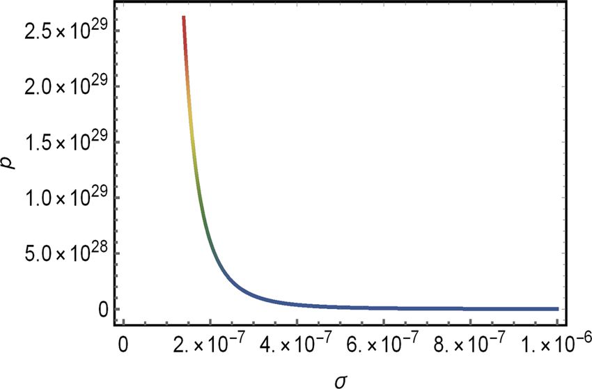
Eur. Phys. J. C (2021) 81:843 Page 3 of 16 843
and, therefore, we can explicitly write down the partition Primarily, let us focus on the mean energy
function in a manner similar to Refs. [23,36] as follows:
ln [Z (β, , σ )]
⎛ √ 16 3 √ 16 3 ⎞
∞
3 2 √ 54 3σ E + 18σ 8 E √ 54 3σ E + 18σ 8 E
V ⎜ 3 4σ +27σ 16 E 4
12 4σ +27σ 16 E 4
12 ⎟
=− ⎝ √ √ + √ √ √ 2/3 ⎠
π2 4/3
0 3 3 4σ 12 + 27σ 16 E 4 + 9σ 8 E 2 3 3 232/3 σ 4 3 4σ 12 + 27σ 16 E 4 + 9σ 8 E 2
(7)
× ln 1 − e−β E
3√ √ 3 2
3 4σ 12 + 27σ 16 E 4 + 9σ 8 E 2
×
3
√ −
3 √ √
dE,
3
232/3 σ 4 3 4σ + 27σ 16 E 4 + 9σ 8 E 2
12
U (β, σ )
⎛ √ 16 3 √ 16 3 ⎞
∞
3 2 √ 54 3σ E + 18σ 8 E √ 54 3σ E + 18σ 8 E
V ⎜ 3 4σ 12 +27σ 16 E 4 4σ 12 +27σ 16 E 4 ⎟
= dE E ⎝ √ √ + √ √ √ 2/3 ⎠
π2 4/3
0 3 3 4σ 12 + 27σ 16 E 4 + 9σ 8 E 2 3 3 232/3 σ 4 3 4σ 12 + 27σ 16 E 4 + 9σ 8 E 2
e−β E
×
1 − e−β E
3√ √ 3 2
3 4σ + 27σ E + 9σ E
12 16 4 8 2
× √ −
3
3 √ √
(9)
3
2·3 σ
2/3 4
3 4σ 12 + 27σ 16 E 4 + 9σ 8 E 2
which implies the following spectral radiance:
χ (σ, ν)
⎛ √ 16 √ 16 ⎞
√ 54 3σ (hν)3 3σ (hν)3
3 2
+ 18σ 8 (hν) √ 54 + 18σ 8 (hν)
hν ⎜
⎜
3 4σ +27σ 16 (hν)4
12
4σ +27σ 16 (hν)4
12 ⎟
⎟
= √ + √ √
π2 ⎝ 4/3 2/3 ⎠
3 3 4σ 12 + 27σ 16 (hν)4 + 9σ 8 (hν)2 3 3 232/3 σ 4 3 4σ 12 + 27σ 16 (hν)4 + 9σ 8 (hν)2
e−β(hν)
×
1 − e−β(hν)
√
3 3 2
3 4σ 12 + 27σ 16 (hν)4 + 9σ 8 (hν)2
×
3
√ − √ . (10)
3
23 σ
2/3 4 3
3 4σ + 27σ (hν) + 9σ (hν)
12 16 4 8 2
where β = 1/(k B T ) is the inverse of the temperature. From
Eq. (7), the thermodynamic functions can be derived. It is Here, E = hν where h is the well-known Planck constant
important to mention that all our calculations will provide and ν is the frequency. Now, let us examine how the param-
the values of these functions per volume V . The thermal eter σ affects the spectral radiance of our theory. In addition,
functions of interest are defined as it must be noted that, despite of showing explicitly the con-
stants h, k B , to obtain the following calculations, we choose
1 ∂ them as being h = k B = 1. At the beginning, we examine
F(β, σ ) = − ln [Z (β, σ )] , U (β, σ ) = − ln [Z (β, σ )] , how the black body spectra can be modified by the parame-
β ∂β
∂ ∂
(8) ter σ . Moreover, we consider three different configurations
S(β, σ ) = k B β 2 F(β, σ ), C V (β, σ ) = −k B β 2 U (β, σ ). of temperatures for our system, namely, CMB (T = 10−13
∂β ∂β
123843 Page 4 of 16 Eur. Phys. J. C (2021) 81:843 Fig. 1 The plots exhibit the spectral radiance χ(ν) changing for dif- dashed) is ascribed to the electroweak configuration, i.e., β = 10−3 ferent values of frequency ν and the Lorentz-breaking parameter σ (its GeV−1 ; the bottom plot shows the black body radiation to the inflation- unit is GeV−1 ). The top left (dotted) is the configuration to the cos- ary period of the Universe, i.e., β = 10−13 GeV−1 mic microwave background, i.e., β = 1013 GeV−1 ; the top right (dot- GeV), electroweak epoch (T = 103 GeV) and inflationary As it can easily be noted, the above expressions are unsolv- era (T = 1013 GeV). able analytically. Thereby, the calculations will be performed The results displayed at Fig. 1 show that the only one numerically. Analogously, we regard the same previous con- configuration of the black body radiation took a proper place figurations of temperature and the plots are exhibited in in a prominent manner (in terms of shape of the curve) – Fig. 2. For the CMB temperature, the curve exhibits a con- it was with the CMB temperature. Furthermore, taking into stant behavior of α. Moreover, to the electroweak epoch, we account the electroweak scenario, we see that the graphics have a decreasing function α̃ when σ started to increase. started to increase reaching maxima peaks and, then, tended The inflationary era, on the other hand, shows an increasing to attenuate their values until having a constant behavior. On function of α̃ for positive changes of σ . To this latter case, the other hand, to the inflationary temperature, the plots show for α̃ < 20, the system seems to show instability. Next, we a behavior closer to Wien’s energy density distribution [37]. shall acquire all the remaining thermodynamic properties in Another interesting aspect to be verified is the correction what follows (Figs. 3, 4). to the Stefan–Boltzmann law ascribed to the parameter σ . In Using the expressions above, we can first obtain the order to do this, let us define the constant: Helmholtz free energy as being α̃ ≡ U (β, σ )β 4 . (11) 123
Eur. Phys. J. C          (2021) 81:843                                                                                     Page 5 of 16   843

Fig. 2 The figure shows the correction to the Stefan–Boltzmann law ascribed to parameter α̃ as a function of σ (its unit is GeV−1 ) for the
temperatures of cosmic microwave background (top left), electroweak scenario (top right) and the early inflationary universe (bottom)

                                                                                    Fig. 4 This figure shows the behavior of the equation of states when
Fig. 3 This figure shows the behavior of the equation of states when
                                                                                    the low temperature limit, namely σβ  1, is taken into account
the high temperature limit, namely σβ  1, is taken into account

                                     ⎛                  √ 16 3                                              √ 16 3                                ⎞
                                ∞
                                             3   2   √ 54 3σ E         + 18σ 8 E                         √ 54 3σ E         + 18σ 8 E
                   V                 ⎜           3    4σ +27σ 16 E 4
                                                         12                                               4σ +27σ 16 E 4
                                                                                                             12                                    ⎟
  F(β, σ ) =                         ⎝     √ √                                           + √            √ √                                     2/3 ⎠
                  βπ 2                                                             4/3
                             0           3  3 4σ 12 + 27σ 16 E 4 + 9σ 8 E 2               3 3 232/3 σ 4  3 4σ 12 + 27σ 16 E 4 + 9σ 8 E 2


                                  3√ √                                    3 2
                                    3 4σ + 27σ E + 9σ E
                                         12         16  4 8 2
      ×ln 1 − e−β E                       √                  −
                                                                             3
                                                                3 √ √
                                                                                                dE,                                                (12)
                                            3
                                              23 σ
                                                2/3   4
                                                                   3 4σ + 27σ 16 E 4 + 9σ 8 E 2
                                                                       12

                                                                                                                                            123
843 Page 6 of 16 Eur. Phys. J. C (2021) 81:843
the entropy
S(β, σ )
⎛ √ 16 3 √ 16 3 ⎞
∞
3 2 √ 54 3σ E + 18σ 8 E √ 54 3σ E + 18σ 8 E
V kB ⎜ 3 4σ +27σ 16 E 4
12 4σ +27σ 16 E 4
12 ⎟
=− ⎝ √ √ + √ √ √ 2/3 ⎠
π2 4/3
0 3 3 4σ 12 + 27σ 16 E 4 + 9σ 8 E 2 3 3 232/3 σ 4 3 4σ 12 + 27σ 16 E 4 + 9σ 8 E 2
×ln 1 − e−β E
3√ √ 3 2
3 4σ + 27σ E + 9σ E
12 16 4 8 2
×
3
√ −
3 √ √
3
232/3 σ 4 3 4σ + 27σ 16 E 4 + 9σ 8 E 2
12
⎛ √ 16 3 √ 16 3 ⎞
3 2
√ 54 3σ E + 18σ 8 E √ 54 3σ E + 18σ 8 E
Vβk B ∞ ⎜ 3 4σ +27σ E
12 16 4 4σ +27σ 16 E 4
12 ⎟
+ 2 E⎝ √ √ + √ √ √ 2/3 ⎠
π 4/3
0 3 3 4σ 12 + 27σ 16 E 4 + 9σ 8 E 2 3 3 232/3 σ 4 3 4σ 12 + 27σ 16 E 4 + 9σ 8 E 2
e−β E
×
1 − e−β E
3√ √ 3 2
3 4σ + 27σ E + 9σ E
12 16 4 8 2
×
3
√ −
3 √ √
dE, (13)
3
23 σ
2/3 4
3 4σ + 27σ 16 E 4 + 9σ 8 E 2
12
and, lastly, the heat capacity
C V (β, σ )
⎛ √ 16 3 √ 16 3 ⎞
∞
3 2 √ 54 3σ E + 18σ 8 E √ 54 3σ E + 18σ 8 E
V kB β2 ⎜ 3 4σ 12 +27σ 16 E 4 4σ 12 +27σ 16 E 4 ⎟
= E2 ⎝ √ √ + √ √ √ 2/3 ⎠
π2 4/3
0 3 3 4σ 12 + 27σ 16 E 4 + 9σ 8 E 2 3 3 232/3 σ 4 3 4σ 12 + 27σ 16 E 4 + 9σ 8 E 2
e−2β E
×
(1 − e−β E )2
3√ √ 3 2
3 4σ + 27σ E + 9σ E
12 16 4 8 2
×
3
√ − 3 √ √
3
232/3 σ 4 3 4σ + 27σ 16 E 4 + 9σ 8 E 2
12
⎛ √ 16 3
3 2
√ 54 3σ E + 18σ 8 E
V kB β2 ∞ 2 ⎜ 3 4σ 12 +27σ 16 E 4
+ E ⎝ √ √
π2 4/3
0 3 3 4σ 12 + 27σ 16 E 4 + 9σ 8 E 2
√ 16 3 ⎞
√ 54 3σ E + 18σ 8E
⎟
4σ 12 +27σ 16 E 4
+ √ √ √ 2/3 ⎠
3 232/3 σ 4
3
3 4σ 12 + 27σ 16 E 4 + 9σ 8 E 2
e−β E
×
1 − e−β E
3√ √ 3 2
3 4σ 12 + 27σ 16 E 4 + 9σ 8 E 2
×
3
√ − √ √ dE. (14)
3
23 σ
2/3 4 3
3 4σ 12 + 27σ 16 E 4 + 9σ 8 E 2
123Eur. Phys. J. C (2021) 81:843 Page 7 of 16 843
Fig. 5 The figure shows the modification of the Helmholtz free energy F(σ ) due to the parameter σ (its unit is GeV−1 ) considering the temperatures
of cosmic microwave background (top left), electroweak scenario (top right) and the early inflationary universe (bottom)
Their behaviors are shown in Figs. 5, 6, and 7 respectively. behavior when σ started to change for both cases as well,
Moreover, the thermal quantities were also calculated [38– i.e., the CMB and the inflationary temperatures. In principle,
43] into different contexts. In the context of CMB, all of this fact might signalize the possibility of some phase tran-
them turned out to have no contribution to our calculations. sition at some large σ ; nevertheless, this hypothesis requires
For Helmholtz free energy, we obtained decreasing curves further investigation.
with an expressive curvature when σ increases for both elec- Whenever we are dealing with the thermodynamic sys-
troweak and inflationary cases. The entropy, on the other tems, one question naturally arises: what is the form of the
hand, showed a decreasing behavior for different values of σ equation of state when the parameter σ , which characterizes
for both electroweak and inflationary cases. It is worth men- the magnitude of Lorentz symmetry breaking, is taken into
tioning that such behavior does not imply an instability since account? To answer such a question, we must start with the
the entropy is still an increasing function when it is analyzed following relation:
against the temperature for fixed values of σ – as it should
dF = −S dT − p dV, (15)
be. Lastly, the heat capacity exhibited a strong increasing
123843 Page 8 of 16 Eur. Phys. J. C (2021) 81:843
Fig. 6 The plots show the modification to the entropy S(σ ) as a function of σ (its unit is GeV−1 ) considering the temperatures of cosmic microwave
background (top left), electroweak scenario (top right), and the early inflationary universe (bottom)
which, immediately, implies
∂F
p=−
∂V T
⎛ √ 16 3
∞
3 2 √ 54 3σ E + 18σ 8 E
1 ⎜ 3 4σ 12 +27σ 16 E 4
= ⎝ √ √
βπ 2 4/3
0 3 3 4σ 12 + 27σ 16 E 4 + 9σ 8 E 2
√ 16 3 ⎞
√ 54 3σ E + 18σ 8 E ⎟
4σ +27σ 16 E 4
12
+ √ √ √ 2/3 ⎠
3 3 232/3 σ 4 3 4σ 12 + 27σ 16 E 4 + 9σ 8 E 2
×ln 1 − e−β E
3√ √ 3 2
3 4σ + 27σ E + 9σ E
12 16 4 8 2
×
3
√ −
3 √ √
dE. (16)
3
232/3 σ 4 3 4σ + 27σ 16 E 4 + 9σ 8 E 2
12
123Eur. Phys. J. C (2021) 81:843 Page 9 of 16 843
Fig. 7 The plots show the modification to the heat capacity C V (σ ) as a function of σ (its unit is GeV−1 ) considering the temperatures of cosmic
microwave background (top left), electroweak scenario (top right), and the early inflationary universe (bottom)
Here, we focus on the study of the behavior of pressure – 3 Thermodynamical aspects of CPT-odd
which leads to the equation of states. After introducing new higher-derivative LV theory
dimensionless variable t = σ E, we get
In this section, let us consider the theory described by the
∞
1 − σβ following dispersion relation [44]:
p= 3 2 dt ln(1 − e t )F(t);
σ βπ 0
t 1 E 2 + αl E 3 + βl Ek2 = k2 + m 2 . (18)
F(t) = 21/6 3−7/6 √ (χ(t))−1/3 + √ (χ(t))1/3
4 + 27t 4
3
18
where l is a parameter characterizing the intensity of the
(χ(t))2/3 − 121/3
· ; Lorentz symmetry breaking. It is clear that in the limit l → 0,
(χ(t))1/3
√ the standard massive dispersion relation E 2 = k2 + m 2 is
χ(t) = 3 · 4 + 27t 4 + 9t 2 . (17) recovered. Such a relation, being similar to relations stud-
ied in Ref. [27], can arise e.g. in a scalar field theory with
With these above expressions, let us examine some limits. the higher-derivative quadratic Lagrangian of the scalar field
Initially, at the very high temperature limit, namely σβ = looking like L = 21 φ( + m 2 + ρ μνλ ∂μ ∂ν ∂ρ )φ, with ρ μνλ
σ T 1, we perform the expansion in the Taylor series. After
1
being a completely symmetric third-rank tensor whose only
∞ yields p =
that, onlythe first two terms are considered, which
β ∞ ch
non-zero components are ρ 000 = βl, and ρ 0i j = 13 αlδ i j . In
1
σ βπ σ 0
3 2 dt F(t)t = σ π4 2 , where c h = 0 dt F(t)t, i.e., principle, it is natural to expect that such a relation, in the
at T → ∞ (β → 0), the pressure tends to a constant. Such massless case, can also arise in a specific higher-derivative
behavior is displayed in Fig. 3; next, at the natural limit of LV extension of QED. In particular, the dispersion relation
low Lorentz symmetry breaking or low temperature, one has displayed in Eq. (18) can be applied to understand how
β
σ 1. In this case, the exponential is strongly∞ suppressed, Planck-scale effects may affect translation transformations.
and one has p = σ 3cβπ l
2 , where cl = 0 dt F(t), i.e., the This is relevant due to the fact that it carries the information
pressure grows linearly with the temperature. Thereby, its on the distance between source and detector, and it factors
corresponding behavior is shown in Fig. 4. in the interplay between quantum-spacetime effects and the
123843 Page 10 of 16 Eur. Phys. J. C (2021) 81:843
Fig. 8 The plots show how the spectral radiance χ̄ (ν) changes as a is ascribed to the electroweak configuration, i.e., β = 10−3 GeV; the
function of frequency ν and l(whose dimension is m · kg −1/2 · s −1 ) for bottom plot shows the black body radiation to the inflationary period of
three different cases. The top left (dotted) is configuration to the cosmic the Universe, i.e., β = 10−13 GeV
microwave background, i.e., β = 1013 GeV; the top right (dot-dashed)
curvature of spacetime [44,45]. In the literature, some propo- ln Z̄ (β, l)
sitions are addressed in the context of gamma-ray-burst neu- ∞ 2 1/2
E + l E3
trinos and photons [46], and IceCube and GRB neutrinos =− 2
π 0 1 − lE
[45].
Thereby, we restrict ourselves to a particular massless (2E + 3l E 2 )(1 − l E) + l(E 2 + l E 3 )
×
case, i.e., we set m = 0, α = 1 and β = 1. In this sense, it is (1 − l E)2
convenient to rewrite Eq. (18) as ×ln 1 − e−β E dE. (21)
E2 + l E3 Using Eq. (21), we can obtain the thermodynamic functions
k2 = , (19)
1 − lE per volume as well. Here, we provide the calculation of
Helmholtz free energy F̄(β, l), mean energy Ū (β, l), entropy
where, analogously with the previous section, the accessible S̄(β, l), and heat capacity C̄ V (β, l). Let us start with the mean
states can be derived: energy
∞ 2 1/2 ∞ 2
E + l E3 1 E + l E3
1/2
¯
(l) = Ū (β, l) = 2 E
2π 2 0 1 − lE π 0 1 − lE
(2E + 3l E 2 )(1 − l E) + l(E 2 + l E 3 ) (2E + 3l E 2 )(1 − l E) + l(E 2 + l E 3 )
× dE. ×
(1 − l E)2 (1 − l E)2
(20) e−β E
× dE, (22)
1 − e−β E
With this, we are able to write down the corresponding par-
tition function as follows which implies the spectral radiance given by:
123Eur. Phys. J. C (2021) 81:843 Page 11 of 16 843
Fig. 9 The figure shows the correction to the Stefan–Boltzmann law represented by parameter ᾱ as a function of l(whose dimension is m · kg−1/2 ·
s−1 ) considering the temperatures of cosmic microwave background (top left), electroweak scenario (top right), and the early inflationary universe
(bottom)
χ̄ (l, ν) consider
1/2
(hν)2 + l(hν)3
= (hν) ᾱ ≡ U (β, l)β 4 . (25)
1 − l(hν)
(2(hν) + 3l(hν)2 )(1 − l(hν)) + l((hν)2 + l(hν)3 )
× The plots are exhibited in Fig. 9 taking differently into
(1 − l(hν))2
account three scenarios, i.e., the temperatures of: CMB, elec-
e−β(hν)
× . (23) troweak epoch and the early inflationary era of the universe.
1 − e−β(hν)
Furthermore, the high-energy limit 2E + 3l E 2 1 − l E is
also regarded. Here, when the CMB temperature is consid-
The respective plots of these thermal quantities are presented
ered, we see a constant behavior of the curve. On the other
in Fig. 8. Here, we show the black body radiation spectra for
hand, to the electroweak scenario, we obtain a monotonically
different values of l corresponding to the Cosmic Microwave
increasing function as l changes. Finally, in the inflationary
Background, electroweak epoch and inflationary era of the
era, we also have a stable model showing a rising behavior
Universe. Moreover, the black body radiation shape is main-
when l increases.
tained for the three of them, differently what happened in
In the same manner, the remaining thermodynamic func-
our first example in the previous section. Note that when
tions can be explicitly computed:
l → 0, we recover the usual radiation constant of the Stefan–
Boltzmann law, namely, u S B = αT 4 . In other words, we have
∞ E2 1/2
∞ 1 + l E3
1 E 3 e−β E π2 F̄(β, l) =
α= 2 dE = . (24) π 2β 0 1 − lE
π 0 1 − e−β E 15
(2E + 3l E 2 )(1 − l E) + l(E 2 + l E 3 )
×
(1 − l E)2
Furthermore, for the sake of examining how the parameter
l affects the correction to the Stefan–Boltzmann law, we also ×ln 1 − e−β E dE, (26)
123843 Page 12 of 16 Eur. Phys. J. C (2021) 81:843
Fig. 10 The figure shows the modification of the Helmholtz free energy F̄ as a function of l(whose dimension is m · kg−1/2 · s−1 ) considering
the temperatures of cosmic microwave background (top left), electroweak scenario (top right), and the early inflationary universe (bottom)
2 1/2
kB ∞ E + l E3 ent scenarios of the Universe: CMB, primordial electroweak
S̄(β, l) = 2 −
π 0 1 − lE epoch, and inflationary era. All these results are demonstrated
in Fig. 10, which displays a trivial contribution to the first
(2E + 3l E )(1 − l E) + l(E 2 + l E 3 )
2
× ln 1 − e−β E case, and a decreasing characteristic for the latter two ones.
(1 − l E)2
2 1/2 Next, we examined the entropy which was shown in Eq. (27);
E + l E3
+E we investigated such thermal function in the same differ-
1 − lE
ent scenarios of the Universe. All these considerations were
(2E + 3l E 2 )(1 − l E) + l(E 2 + l E 3 ) e−β E
dE, shown in Fig. 11, which exhibited the same trivial contribu-
(1 − l E)2 1 − e−β E
tion to the first case, despite of showing an increase char-
kB β2 ∞ acteristic to the latter two ones. Finally, we studied the heat
C̄ V (β, l) = dE
π2 0 capacity exhibited in Eq. (27); we also examined this ther-
1/2
E2 + l E3 mal function in the same different scenarios of the Universe.
× E2
1 − lE All these considerations were shown in Fig. 12, exhibiting
(2E + 3l E 2 )(1 − l E) + l(E 2 + l E 3 ) e−2β E a trivial contribution to the first case as well, and increasing
× 2 curves for the next two ones.
(1 − l E)2 1 − e−β E
2 Here, just as we did in the previous section, we also present
3 1/2
2 E + lE the analysis of the equation of state. Moreover, since there
+E
1 − lE is no analytical solution to perform our analysis, we have to
(2E + 3l E 2 )(1 − l E) + l(E 2 + l E 3 ) e−β E consider a particular limit to obtain its magnitude as we did
× .
(1 − l E)2 1 − e−β E before. The limit that we study is (E 2 +l E 3 )1/2 /(1−l E)2
(27) 1. With it, we obtain the following expression
Initially, we provide the analysis of the Helmholtz free energy 1 4 l 1
displayed in Eq. (26); it is considered within three differ- p= T 270l ζ (5) + 4π
6 2
+ 90 2 ζ (3) . (28)
45π 2 T T
123Eur. Phys. J. C (2021) 81:843 Page 13 of 16 843
Fig. 11 The figure shows the modification of the entropy S̄ as a function of l(whose dimension is m · kg−1/2 · s−1 ) considering the temperatures
of cosmic microwave background (top left), electroweak scenario (top right) and the early inflationary universe (bottom)
The behavior of Eq. (28) is displayed in Fig. 13. Differently We calculated the modification to the black body radi-
with what happens to the model involving σ , the dispersion ation spectra and to the Stefan–Boltzmann law due to the
relation coming from Eq. (18) has a fascinating feature: the parameters σ and l. For these theories, we explicitly obtained
shape exhibited to the equation of states turns out to be sensi- the corresponding equation of states and the thermodynamic
tive to the modification of the values of l. Furthermore, note functions as well, i.e., the mean energy, the Helmholtz free
that, if we consider l → 0, we obtain energy, the entropy, and the heat capacity. Moreover, all the
calculations presented in this work were performed taking
90ζ (3) 4
p= T . (29) into account three different scenarios of the Universe: cosmic
45π 2
microwave background, electroweak epoch, and inflationary
era.
Furthermore, since the heat capacity rapidly increased
with the Lorentz-breaking parameters at high temperatures,
4 Conclusion perhaps one might expect a phase transition in those sce-
narios. Nevertheless, a further investigation in this direction
We considered the thermodynamical aspects of two higher- might be accomplished in order to provide a proper exam-
derivative Lorentz-breaking theories, namely, CPT-even and ination. Thereby, as a further perspective, we suggest the
CPT-odd ones. Within our study, we focused on the disper- detailed study of the whole field of Horava–Lifshitz grav-
sion relations rather than the specific form of the Lagrangians. ity model and the possible phase transitions in our models.
In this way, we expect that our results can be applied not only Another feasible continuation of this study can consist in its
to scalar field models as we assumed, but also to specific application to other higher-derivative Lagrangians of certain
gauge or spinor field theories. known field theories, f.e. those ones discussed in [15].
123843 Page 14 of 16 Eur. Phys. J. C (2021) 81:843 Fig. 12 The figure shows the modification of the heat capacity C̄ V as a function of l(whose dimension is m · kg−1/2 · s−1 ) considering the temperatures of cosmic microwave background (top left), electroweak scenario (top right) and the early inflationary universe (bottom) Fig. 13 The figure shows the equation of states for different values of p, T , and l(whose dimension is m · kg−1/2 · s−1 ) 123
Eur. Phys. J. C       (2021) 81:843                                                                                Page 15 of 16     843

Acknowledgements The authors would like to thank the Conselho               12. R.C. Myers, M. Pospelov, Ultraviolet modifications of dispersion
Nacional de Desenvolvimento Científico e Tecnológico (CNPq) for                 relations in effective field theory. Phys. Rev. Lett. 90(21), 211601
financial support and L. L. Mesquita for the careful reading of this            (2003)
manuscript and for the suggestions given to us. The work by A. Yu. P.       13. V.A. Kosteleckỳ, M. Mewes, Electrodynamics with Lorentz-
has been partially supported by the CNPq project No. 301562/2019-9.             violating operators of arbitrary dimension. Phys. Rev. D 80(1),
Particularly, A. A. Araújo Filho acknowledges the Facultad de Física-           015020 (2009)
Universitat de València and Gonzalo J. Olmo for the kind hospitality        14. V.A. Kosteleckỳ, Z. Li, Gauge field theories with Lorentz-violating
when this work was made. Moreover, A. A. Araújo Filho has been par-             operators of arbitrary dimension. Phys. Rev. D 99(5), 056016
tially supported by Conselho Nacional de Desenvolvimento Científico             (2019)
e Tecnológico (CNPq)-142412/2018-0, and CAPES-PRINT (PRINT-                 15. T. Mariz, J. Nascimento, A.Y. Petrov, C.M. Reyes, Quantum aspects
PROGRAMA INSTITUCIONAL DE INTERNACIONALIZAÇÃO)-                                 of the higher-derivative Lorentz-breaking extension of qed. Phys.
88887.508184/2020-00.                                                           Rev. D 99(9), 096012 (2019)
                                                                            16. D. Colladay, P. McDonald, Statistical mechanics and Lorentz vio-
Data Availability Statement This manuscript has no associated data              lation. Phys. Rev. D 70(12), 125007 (2004)
or the data will not be deposited. [Authors’ comment: Data sharing          17. R. Casana, M.M. Ferreira Jr., J.S. Rodrigues, Lorentz-violating
not applicable to this article as no datasets were generated or analysed        contributions of the Carroll-field-Jackiw model to the CMB
during the current study.]                                                      anisotropy. Phys. Rev. D 78(12), 125013 (2008)
                                                                            18. R. Casana, M.M. Ferreira Jr., J.S. Rodrigues, M.R. Silva, Finite
Open Access This article is licensed under a Creative Commons Attri-            temperature behavior of the c p t-even and parity-even electro-
bution 4.0 International License, which permits use, sharing, adaptation,       dynamics of the standard model extension. Phys. Rev. D 80(8),
distribution and reproduction in any medium or format, as long as you           085026 (2009)
give appropriate credit to the original author(s) and the source, pro-      19. M. Gomes, T. Mariz, J. Nascimento, A. Petrov, A. Santos, A. da
vide a link to the Creative Commons licence, and indicate if changes            Silva, Free energy of Lorentz-violating qed at high temperature.
were made. The images or other third party material in this article             Phys. Rev. D 81(4), 045013 (2010)
are included in the article’s Creative Commons licence, unless indi-        20. A.A. Araújo Filho, Lorentz-violating scenarios in a thermal reser-
cated otherwise in a credit line to the material. If material is not            voir. Eur. Phys. J. Plus 136, 417 (2021). https://doi.org/10.1140/
included in the article’s Creative Commons licence and your intended            epjp/s13360-021-01434-8
use is not permitted by statutory regulation or exceeds the permit-         21. A.A. Araújo Filho, R.V. Maluf, Thermodynamic properties in
ted use, you will need to obtain permission directly from the copy-             higher-derivative electrodynamics. Brazilian J. Phys. 51, 820–830
right holder. To view a copy of this licence, visit http://creativecomm         (2021). https://doi.org/10.1007/s13538-021-00880-0
ons.org/licenses/by/4.0/.                                                   22. A.A. Filho, J. Reis, Thermal aspects of interacting quantum gases in
Funded by SCOAP3 .                                                              Lorentz-violating scenarios. Eur. Phys. J. Plus 136(3), 1–30 (2021)
                                                                            23. M. Anacleto, F. Brito, E. Maciel, A. Mohammadi, E. Passos, W.
                                                                                Santos, J. Santos, Lorentz-violating dimension-five operator con-
                                                                                tribution to the black body radiation. Phys. Lett. B 785, 191–196
                                                                                (2018)
                                                                            24. S. Das, S. Ghosh, D. Roychowdhury, Relativistic thermodynamics
References                                                                      with an invariant energy scale. Phys. Rev. D 80(12), 125036 (2009)
                                                                            25. A.A. Araújo Filho, A. Yu. Petrov, Bouncing universe in a heat bath
 1. S. Liberati, L. Maccione, Astrophysical constraints on Planck scale         (2021). arXiv: 2105.05116
    dissipative phenomena. Phys. Rev. Lett. 112(15), 151301 (2014)          26. A.A. Araújo Filho, J.A.A.S. Reis, S. Ghosh. Fermions on a torus
 2. J.D. Tasson, What do we know about Lorentz invariance? Rep.                 knot (2021). arXiv: 2108.07336
    Progr. Phys. 77(6), 062901 (2014)                                       27. G. Amelino-Camelia, Testable scenario for relativity with mini-
 3. A. Hees, Q.G. Bailey, A. Bourgoin, P.-L. Bars, C. Guerlin, L.               mum length. Phys. Lett. B 510(1–4), 255–263 (2001)
    Poncin-Lafitte et al., Tests of Lorentz symmetry in the gravitational   28. S. Bianco, V.N. Friedhoff, E. Wilson-Ewing, Modified disper-
    sector. Universe 2(4), 30 (2016)                                            sion relations, inflation, and scale invariance. Phys. Rev. D 97(4),
 4. R. Maluf, A.A. Filho, W. Cruz, C. Almeida, Antisymmetric tensor             046006 (2018)
    propagator with spontaneous Lorentz violation. EPL (Europhysics         29. M. Gomes, F. Marques, T. Mariz, J. Nascimento, A.Y. Petrov, A.
    Letters) 124(6), 61001 (2019)                                               da Silva, One-loop corrections in the z= 3 lifshitz extension of qed.
 5. J. Alfaro, H.A. Morales-Tecotl, L.F. Urrutia, Loop quantum gravity          Phys. Rev. D 98(10), 105016 (2018)
    and light propagation. Phys. Rev. D 65(10), 103509 (2002)               30. P. Horava, Quantum gravity at a Lifshitz point. Phys. Rev. D 79,
 6. M. Pospelov, Y. Shang, Lorentz violation in hořava-lifshitz-type           084008 (2009)
    theories. Phys. Rev. D 85(10), 105001 (2012)                            31. K. de Farias, T. Sampaio, M. Anacleto, F. Brito, E. Passos, Lifshitz-
 7. N.E. Mavromatos, Lorentz invariance violation from string theory            scaling in CPT-even Lorentz-violating electrodynamics and GRB
    (2007). arXiv preprint arXiv:0708.2250                                      time delay. Eur. Phys. J. Plus 136(2), 257 (2021)
 8. S.M. Carroll, J.A. Harvey, V.A. Kosteleckỳ, C.D. Lane, T.              32. F. Reif, Fundamentals of statistical and thermal physics (1998)
    Okamoto, Noncommutative field theory and Lorentz violation.             33. J.W. Gibbs, Elementary Principles in Statistical Mechanics
    Phys. Rev. Lett. 87(14), 141601 (2001)                                      (Courier Corporation, Chelmsford, 2014)
 9. V.A. Kosteleckỳ, N. Russell, Data tables for Lorentz and c p t         34. W. Greiner, L. Neise, H. Stöcker, Thermodynamics and Statistical
    violation. Rev. Mod. Phys. 83(1), 11 (2011)                                 Mechanics (Springer Science & Business Media, Berlin, 2012)
10. J. Collins, A. Perez, D. Sudarsky, L. Urrutia, H. Vucetich, Lorentz     35. H.B. Callen, Thermodynamics and an introduction to thermostatis-
    invariance and quantum gravity: an additional fine-tuning problem?          tics (1998)
    Phys. Rev. Lett. 93(19), 191301 (2004)                                  36. R. Maluf, D. Dantas, C. Almeida, The Casimir effect for the scalar
11. J. Nascimento, A.Y. Petrov, C.M. Reyes, Renormalization in a                and Elko fields in a Lifshitz-like field theory. Eur. Phys. J. C 80,
    Lorentz-violating model and higher-order operators. Eur. Phys. J.           1–10 (2020)
    C 78(7), 7–578 (2018)                                                   37. N. Zettili, Quantum mechanics: concepts and applications (2003)

                                                                                                                                        123
843 Page 16 of 16 Eur. Phys. J. C (2021) 81:843
38. R.R. Oliveira, A.A.A. Filho, F.C. Lima, R.V. Maluf, C.A. Almeida, 43. G. Amelino-Camelia, F. Brighenti, G. Gubitosi, G. Santos, Thermal
Thermodynamic properties of an Aharonov–Bohm quantum ring. dimension of quantum spacetime. Phys. Lett. B 767, 48–52 (2017)
Eur. Phys. J. Plus 134(10), 495 (2019) 44. G. Rosati, G. Amelino-Camelia, A. Marciano, M. Matassa, Planck-
39. R. Oliveira, A.A. Filho, Thermodynamic properties of neutral dirac scale-modified dispersion relations in frw spacetime. Phys. Rev. D
particles in the presence of an electromagnetic field. Eur. Phys. J. 92(12), 124042 (2015)
Plus 135(1), 99 (2020) 45. G. Amelino-Camelia, L. Barcaroli, G. D’Amico, N. Loret, G.
40. J. Reis et al., How does geometry affect quantum gases? (2020). Rosati, Icecube and grb neutrinos propagating in quantum space-
arXiv preprint: arXiv:2012.13613 time. Phys. Lett. B 761, 318–325 (2016)
41. I. Lobo, V. Bezerra, J.M. Graça, L.C. Santos, M. Ronco, Effects of 46. G. Amelino-Camelia, G. D’Amico, G. Rosati, N. Loret, In vacuo
planck-scale-modified dispersion relations on the thermodynamics dispersion features for gamma-ray-burst neutrinos and photons.
of charged black holes. Phys. Rev. D 101(8), 084004 (2020) Nat. Astron. 1(7), 1–6 (2017)
42. I. Lobo, G. Santos, Thermal dimensional reduction and black hole
evaporation (2020). arXiv preprint arXiv:2009.08556
123You can also read