Heating of the solar chromosphere in a sunspot light bridge by
←
→
Page content transcription
If your browser does not render page correctly, please read the page content below
A&A 652, L4 (2021)
https://doi.org/10.1051/0004-6361/202141456                                                                         Astronomy
c ESO 2021                                                                                                           &
                                                                                                                    Astrophysics

                                                         LETTER TO THE EDITOR

    Heating of the solar chromosphere in a sunspot light bridge by
                            electric currents
          Rohan E. Louis1 , Avijeet Prasad2 , Christian Beck3 , Debi P. Choudhary4 , and Mehmet S. Yalim2

      1
          Udaipur Solar Observatory, Physical Research Laboratory, Dewali Badi Road, Udaipur 313001, Rajasthan, India
          e-mail: rlouis@prl.res.in
      2
          Center for Space Plasma and Aeronomic Research, The University of Alabama in Huntsville, Huntsville, AL 35899, USA
      3
          National Solar Observatory (NSO), 3665 Discovery Drive, Boulder, CO 80303, USA
      4
          Department of Physics and Astronomy, California State University, Northridge (CSUN), Northridge, CA 91330-8268, USA

     Received 2 June 2021 / Accepted 13 July 2021

                                                                 ABSTRACT

     Context. Resistive Ohmic dissipation has been suggested as a mechanism for heating the solar chromosphere, but few studies have
     established this association.
     Aims. We aim to determine how Ohmic dissipation by electric currents can heat the solar chromosphere.
     Methods. We combine high-resolution spectroscopic Ca ii data from the Dunn Solar Telescope and vector magnetic field observations
     from the Helioseismic and Magnetic Imager (HMI) to investigate thermal enhancements in a sunspot light bridge. The photospheric
     magnetic field from HMI was extrapolated to the corona using a non-force-free field technique that provided the three-dimensional
     distribution of electric currents, while an inversion of the chromospheric Ca ii line with a local thermodynamic equilibrium and a non-
     local thermodynamic equilibrium spectral archive delivered the temperature stratifications from the photosphere to the chromosphere.
     Results. We find that the light bridge is a site of strong electric currents, of about 0.3 A m−2 at the bottom boundary, which extend
     to about 0.7 Mm while decreasing monotonically with height. These currents produce a chromospheric temperature excess of about
     600−800 K relative to the umbra. Only the light bridge, where relatively weak and highly inclined magnetic fields emerge over a
     duration of 13 h, shows a spatial coincidence of thermal enhancements and electric currents. The temperature enhancements and the
     Cowling heating are primarily confined to a height range of 0.4−0.7 Mm above the light bridge. The corresponding increase in internal
     energy of 200 J m−3 can be supplied by the heating in about 10 min.
     Conclusions. Our results provide direct evidence for currents heating the lower solar chromosphere through Ohmic dissipation.
     Key words. sunspots – Sun: chromosphere – Sun: corona – Sun: photosphere – Sun: magnetic fields

1. Introduction                                                           formation of current sheets when a discontinuity in the three-
                                                                          dimensional (3D) magnetic field arises (Solanki et al. 2003;
The solar chromosphere serves as an important conduit for mass            Bahauddin et al. 2021). Such currents are often seen in sunspot
and energy between the dense, 6000 K photosphere and the                  light bridges (LBs) and δ spots (Jurčák et al. 2006; Shimizu et al.
tenuous, million degree corona. The solar chromosphere has a
                                                                          2009; Balthasar et al. 2014; Toriumi et al. 2015a; Robustini et al.
complex magnetic structure, where the plasma beta changes dra-
                                                                          2018). However, estimates of the current density are typically
matically (Gary 2001). Determining the processes that maintain
the thermal structure of the solar atmosphere is one of the funda-        confined to the solar photosphere and only provide the vertical
mental problems in solar physics (Narain & Ulmschneider 1996).            component of the current Jz , while Socas-Navarro (2005) found
     The energy transfer in the chromosphere can be attributed to         only a weak correlation between currents and chromospheric
a number of mechanisms, such as Alfv́en waves (Osterbrock                 heating. In this article, we combine non-force-free field (NFFF)
1961; Stein 1981; van Ballegooijen et al. 2011; Shelyag et al.            extrapolations with thermal inversions to study intense electric
2016; Grant et al. 2018; Sakaue & Shibata 2020), spicules                 currents and strong chromospheric temperature enhancements
(Beckers 1968; Pneuman & Kopp 1978; Athay & Holzer 1982;                  over a sunspot, which occur as a result of large-scale magnetic
De Pontieu et al. 2009; Beck et al. 2016), nanoflares (Priest             flux emergence in an LB.
et al. 2018; Syntelis & Priest 2020), and magneto-acoustic shocks
(De Pontieu et al. 2015). Some authors have suggested that the            2. Observations
heating of the chromosphere is due to the dissipation of acoustic
waves (Ulmschneider et al. 1978; Kalkofen 2007), although this            We analyzed observations of the leading sunspot in NOAA
has been questioned by Athay & Holzer (1982) and Beck et al.              AR 12002 (Fig. 1a) on 2014 March 13 from 20:44 to 21:00 UT,
(2009, 2012).                                                             combining data from the Helioseismic and Magnetic Imager
     Another candidate for heating the solar chromosphere is              (HMI; Schou et al. 2012) on board the Solar Dynamics Obser-
resistive Ohmic dissipation (Parker 1983; Tritschler et al. 2008).        vatory (SDO; Pesnell et al. 2012) and the Interferometric
The occurrence of dynamic phenomena in the chromosphere and               BI-dimensional Spectrometer (IBIS; Cavallini 2006) at the
transition region has been attributed to plasma heating by the            Dunn Solar Telescope (DST). The SDO data comprise two

                                                      Article published by EDP Sciences                                           L4, page 1 of 6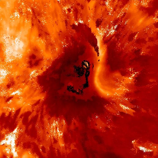
A&A 652, L4 (2021)

Fig. 1. HMI and IBIS observations of the leading sunspot in NOAA AR 12002. Top: full-disk HMI continuum image (left) at 21:00 UT on 2014
March 13, IBIS Ca ii IR line-core image (middle), and speckle-reconstructed IBIS broadband image (right). The square and dashed rectangle in
panel a indicate the IBIS and HMI SHARP FOV, respectively. Bottom: field lines derived from the NFFF extrapolation overlaid on a composite
image of the vertical component of the magnetic field and the AIA 171 Å image for the SHARP FOV. The solid and dashed white squares
correspond to the IBIS FOV and the smaller FOV shown in Fig. 2, respectively.

Spaceweather HMI Active Region Patch (SHARP) maps of the                890 ± 50 G, and 850 ± 55 G, respectively. The uncertainty in the
vector magnetic field at 20:48 UT and 21:00 UT. IBIS acquired           current density was determined by using the deviation between
spectral scans in the Ca ii IR line at 854 nm with a spatial sam-       the extrapolated and observed horizontal magnetic field, which
pling of 000. 1 px−1 across a 9000 circular field of view (FOV). Only   yielded a mean error of 1.6 × 10⁻² A m−2 , 1.5 × 10⁻² A m−2 , and
the two scans at 20:44 UT and 20:55 UT were used here. The              5.0 × 10⁻³ A m−2 in J x , Jy , and Jz , respectively, within the LB.
DST setup and data are described in detail in Louis et al. (2020),      These values translate into relative errors of 33%, 27%, and 16%,
hereafter LBC20.                                                        respectively, and pertain to the HMI sampling of 000. 5. The fric-
                                                                        tional Joule heating profile was calculated from the dissipation
3. Data analysis                                                        of currents perpendicular to the magnetic field through the Cowl-
                                                                        ing resistivity ηC (Yalim et al. 2020), where ηC is a function of
To infer the magnetic connectivity, we used the NFFF extrap-            the magnetic field B, plasma bulk density ρ, and temperature T
olation technique (Hu & Dasgupta 2008; Hu et al. 2008,                  as well as the ion and electron number densities ni and ne in
2010), where the magnetic field is described by the double-curl         the chromosphere. All values of physical quantities, apart from
Beltrami equation derived from a variational principle of the           B, were taken from the tabulated data of the Maltby-M umbral
minimum energy dissipation rate (Bhattacharyya et al. 2007).            core model (Maltby et al. 1986). We discarded the Coulomb
This method is well suited to the high plasma-β photospheric            resistivity because it is two to three orders of magnitude smaller
boundary (Gary 2001) and has been successfully used in many             than ηC (see Fig. 3 of Yalim et al. 2020) and only retained
recent studies (Nayak et al. 2019; Liu et al. 2020; Yalim et al.        the Cowling heating: ηC J⊥2 , where J⊥ is the component of the
2020; Prasad et al. 2020). The extrapolation provides the mag-          current perpendicular to the magnetic field. The relative error
netic field vector B(x, y, z), from which we derived the total          in the Joule heating was about 34%, corresponding to about
(|J|), vertical (Jz ), and horizontal (Jhor ) current densities. The    0.06 W m−3 in the LB.
mean values of Bx , By , and Bz in the LB and their errors,                 The IBIS spectra were inverted with both the local ther-
as derived from the HMI SHARP maps, were 525 ± 45 G,                    modynamic equilibrium (LTE) and non-LTE (NLTE) version of

L4, page 2 of 6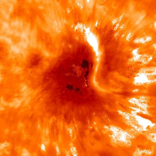
R. E. Louis et al.: Heating of the solar chromosphere in a sunspot by electric currents

                                                                                                Fig. 2. Electric currents, temperature enhance-
                                                                                                ments, and Joule heating in the sunspot LB.
                                                                                                Panels 1a–1d: spatial distribution of the ver-
                                                                                                tical current density Jz and horizontal cur-
                                                                                                rent density Jhor at z = 0.36 Mm (top) and
                                                                                                z = 0.72 Mm (bottom). The horizontal lines
                                                                                                in panel 1b indicate the locations of the 2D
                                                                                                cuts shown in Fig. 4. The white horizontal line
                                                                                                marks cut No. 5 used in Figs. 4g and h. Panels
                                                                                                2a–2b: spatial distribution of the vertical (top)
                                                                                                and horizontal (bottom) component of the mag-
                                                                                                netic field at z = 0.36 Mm. Panels 2c–2d: spa-
                                                                                                tial distribution of the NLTE temperature at
                                                                                                z = 0.36 Mm (top) and z = 0.72 Mm (bottom).
                                                                                                The white rectangle in panel 2c is a smaller
                                                                                                FOV centered on the LB shown in Fig. 3. Pan-
                                                                                                els 3a–3d and 4a–4d: spatial distribution of J|| ,
                                                                                                J⊥ , Cowling resistivity ηC , and its associated
                                                                                                Joule heating. The color bar in panels 4 com-
                                                                                                prises two scales, where the top and bottom
                                                                                                numbers correspond to 0.36 Mm and 0.72 Mm,
                                                                                                respectively.

the CAlcium Inversion based on a Spectral ARchive (CAISAR;              The LB formed as a result of large-scale magnetic flux emer-
Beck et al. 2015, 2019) code. Individual spectra are inverted on        gence in the sunspot over a duration of 13 h, which was seen as
a pixel-by-pixel basis. The model atmospheres in the archives           strong blueshifts of about 1 km s−1 all along the body of the LB
are in hydrostatic equilibrium. The resulting temperature strat-        (LBC20). The LB comprised weak and highly inclined magnetic
ifications were converted from optical depth to geometrical             fields, with a mean field strength and inclination of about 1.5 kG
height based on the Harvard Smithsonian reference atmosphere            and 55◦ , respectively, while in the southern part of the structure
(Gingerich et al. 1971) without considering lateral pressure equi-      the values are about 1.2 kG and 85◦ , respectively. The LB has
librium. The temperature maps were then spatially de-projected          a pronounced curvature that connects the southern and north-
to the local reference frame to match the HMI SHARP mag-                western penumbral sections (panel c). Figure 1d shows the coro-
netic field in x and y. The LTE and NLTE temperature excess,            nal magnetic field from the NFFF extrapolation overlaid on a
estimated with respect to the mean umbral temperature, were             composite of the Atmospheric Imaging Assembly (AIA, Lemen
subsequently converted to the increase in internal energy as in         et al. 2012) 171 Å image and Bz . Prominent loops connect the
Eq. (1) of Beck et al. (2013), see also Rezaei & Beck (2015),           sunspot to the opposite polarity to the east, while the field lines
their Sect. 4.7. For a partially ionized gas, this value serves as      in the western part of the sunspot are mostly open. No loops were
the lower limit since the product of the ionization fraction and        found to follow the LB structure, but a few field lines directly
the ionization potential per unit mass is an additional term in         neighboring the LB showed a small dent away from the LB for
the internal energy. The error in temperature is 20−100 K for           z < 1 Mm.
−5 < log τ < −2, with nearly identical temperatures in LTE and
NLTE for log τ > −2 (LBC20, Sect. 3.3).
                                                                        4.2. Electric current density and temperature
4. Results                                                              Figure 2 shows that both the current density and temperature are
                                                                        larger over the LB than anywhere else in the sunspot at 21:00 UT.
4.1. Global topology of NOAA AR 12002
                                                                        At the bottom boundary the total current |J| reaches a maximum
Figure 1b shows the sunspot in the chromospheric Ca ii spec-            value of 0.3 A m−2 with a mean value of 0.11 A m−2 . The total
tral line, with a strong brightness enhancement all along the LB.       current is dominated by Jhor , which is three times stronger than

                                                                                                                                 L4, page 3 of 6
A&A 652, L4 (2021)
Jz . At z = 0.36 Mm, the maximum values of Jz and Jhor reduce to
0.05 A m−2 and 0.13 A m−2 , respectively. At the same height, the
entire length of the LB is hotter than the surroundings, with LTE
and NLTE temperatures of 4700 K and 4900 K, respectively. At
the southern end of the LB, the temperature reaches 5270 K
and 6775 K in LTE and NLTE, respectively. The LB is nearly
600−800 K hotter than the neighboring umbra. Panels 3 and 4 of
Fig. 2 show that the components of the currents parallel (J|| ) and
perpendicular (J⊥ ) to the magnetic field are about 0.04 A m−2
in the LB at a height of 0.36 Mm and reduce by about 60% at
0.72 Mm. The ηC increases by a factor of five from 0.36 Mm to
0.72 Mm, although it is weaker in the LB relative to the umbra,
by a factor of about 1.7, owing to its B2 dependence on the mag-
netic field strength. The Joule heating due to ηC is about 1 W m−3
at 0.72 Mm.
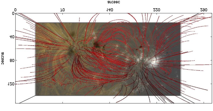
Figure 3 shows that the temperature enhancement along the
spine of the LB is flanked by intense currents that have opposite
signs in Jz . The Jhor , depicted with arrows, is parallel to the LB
spine, with opposite directions on either side. Nearly identical
properties were found for the second data set at 20:48 UT.
Panels a–e of Fig. 4 show 2D x−z plots of different physi-
cal parameters along the cuts across the LB indicated in panel
2b of Fig. 2. The bottom and top panels (i.e., 1a and 13a) corre-
spond to the cut at the southern and northern end, respectively.
Both current and temperature enhancements follow the location
Fig. 3. Distribution of electric currents around the temperature enhance-
of the spine of the LB along its extent. As already seen in Figs. 2
ments in the LB. Left: horizontal current vectors overlaid on the NLTE
and 3, the LB is hottest at its southern end (panels 1–4), with temperature map at 0.36 Mm for the FOV depicted with the white rect-
temperature decreasing towards its northern end. The tempera- angle in Fig. 2 (panel 1a). Arrows have been drawn for every pixel
ture enhancement is seen in both LTE and NLTE, although in where |Jz | is greater than 0.01 A m−2 . Right: horizontal current vectors
NLTE the enhancement is much hotter and narrower, confined overlaid on Jz at 0 Mm.
to a height between 0.2 and 0.6 Mm (panels 1d–5d and 1e–5e in
Fig. 4). The Joule heating (panel c) also exhibits the same spatial
variation along the spine of the LB. However, the heating is con- Joule heating over height as described in the previous section.
fined to a narrow height range at about 0.7 Mm (panels 3c–9c) To cover the spatial extent of the LB, we moved the location
because of the vertical stratification of ηC . of these cuts in steps of one pixel from south to north. The left
The height extent of the different quantities is better seen panel of Fig. 5 reveals that the total current |J| is strongly pos-
in Fig. 4f, which shows the stratification of T , |J|, and heat- itively correlated with the temperature, exhibiting a Spearman
ing for cut No. 5. The NLTE temperature has a sharp peak of coefficient of 0.75 and 0.73 for the LTE and NLTE case, respec-
up to 2000 K of 0.4 Mm width at a height of 0.42 Mm, while tively. The scatter plots between the increase in internal energy
the LTE temperature shows a broader, lower enhancement of over the neighboring umbra and the Joule heating (right panel of
800 K over a larger height range. The current drops monotoni- Fig. 5) also exhibit a high correlation, with values of 0.75 and
cally with height, while the heating shows a sharp peak, simi- 0.7 for the LTE and NLTE case, respectively.
lar to the NLTE temperature but at a slightly higher altitude of The ratio of the increase in internal energy and the Joule
0.72 Mm. heating provides the timescale over which the currents must dis-
Figure 4g, with height-averaged T , |J|, and heating val- sipate in order to produce the observed temperature enhance-
ues for the same cut, confirms once more that the largest cur- ments. The dissipative timescale is about 10 min, with both the
rents flank the LB spine, while the temperature enhancements LTE and NLTE cases having a nearly identical slope in the lin-
are co-spatial with the Joule heating at the center of the LB. ear fit. This is consistent with the lifetime of the currents that
The temperature, current, and heating were averaged in height are permanently present from 20:36 UT to 21:00 UT. The excess
between 0.18−0.6 Mm, 0−0.36 Mm, and 0−0.72 Mm, respec- emission in the Ca ii IR line core in the LB relative to the quiet
tively. Figure 4h shows the heating to be highest at the LB as Sun amounted to only about 6 × 10⁻³ W m−3 at a characteristic
J⊥ has a maximum value due to the large field inclination in heating rate of 0.2 W m−3 . Radiative losses should thus have no
the LB even if ηC decreases slightly. The J⊥2 dependence of the strong impact on the timescale.
Joule heating renders it a factor of six higher in the LB than the
adjacent umbra. Similar currents and heating were already
present at 20:36 UT, about 10 min prior to the DST observations. 5. Discussion
4.3. Ohmic dissipation in the LB We find that the LB is hotter than the rest of the sunspot,
both spatially and vertically. The temperature enhancement is
While Figs. 2 and 3 demonstrate the spatial association of the driven by intense electric currents, with the horizontal compo-
currents and Joule heating with temperature, Fig. 5 shows the nent dominating the vertical current. The maximum value of
scatter plots of currents, heating, and temperature. The scatter Jz at z = 0 Mm is about 0.1 A m−2 , which is consistent with
plots were constructed by taking a 13-pixel-wide horizontal cut, Toriumi et al. (2015a). These values are about a factor of two
centered on the location of maximum temperature on the LB smaller than those reported by Jurčák et al. (2006), Balthasar
spine, and then averaging temperature, the total current, and the (2006), and Shimizu et al. (2009), which could be due to the HMI
L4, page 4 of 6R. E. Louis et al.: Heating of the solar chromosphere in a sunspot by electric currents
Fig. 4. Vertical variation in physical parameters at different positions on the spine of the LB. Columns a–e: 2D slices of the currents Jz and Jhor ,
Joule heating by Cowling resistivity, LTE temperature T , and NLTE temperature T (left to right) for the horizontal cuts across the LB (panel 2b
in Fig. 2). Panel f: vertical distribution of parameters at the center of the LB at the white horizontal cut shown in Fig. 2b. The heating term has
been scaled down by a factor of five. Panel g: horizontal variation in parameters along the same cut after temperature, current, and heating were
averaged in height. The heating term has been reduced by a factor of two. Panel h: same as above but for J⊥ , ηC , and the Joule heating. J⊥ has
been scaled up by a factor of three.
Fig. 5. Correlation between currents and temperature enhancements as well as Joule heating and increase in internal energy in the LB. Left: scatter
plots of |J| and temperature. The pluses and open circles correspond to the LTE and NLTE case, respectively. The red and black colors correspond
to the data set at 20:48 UT and 21:00 UT, respectively. The solid black line and the grey line are a linear fit to the scatter in the NLTE and LTE
case, respectively. The Spearman correlation coefficient for the NLTE case is shown in the lower right corner, while the LTE value is enclosed in
parentheses. The dotted and dashed lines correspond to the average umbral and quiet Sun temperature, respectively. Right: scatter plots of Joule
heating and internal energy. The mean error associated with the different parameters in the LB is shown in the top right corner of each panel.
spatial resolution in our case being insufficient to resolve cur- a good indicator for locations, with a strong correlation between
rent sheets. The true currents are expected to be larger than currents and temperature enhancements. While the strong cor-
the values derived. The |J| had maximum and mean values of relation between currents and increased temperature is seen for
0.2 and 0.14 A m−2 , respectively, in the penumbra in Puschmann most of the LB spine, the strongest temperature enhancements
et al. (2010). The large values of 0.3 A m−2 estimated in the LB at the southern end of the LB are associated with weaker cur-
arise from the emergence of a relatively weak, nearly horizon- rents (Figs. 2 and 3). This suggests that the heating mechanism
tal magnetic structure in the sunspot over a duration of at least in the LB could be more intricate than just a strongly localized
13 h (LBC20). As a consequence of the sustained emergence of current dissipation with an instant temperature rise. The com-
horizontal magnetic fields, one would expect the correspond- plex structure of the LB and its emerging magnetic flux (which is
ing temperature enhancements to likely be present over a sim- not fully resolved in the HMI data), the magnetic field extrapola-
ilar timescale. The value of the current density in the rest of the tion, directed mass flows, heat conduction, and possible time lags
sunspot is consistent with the results of Socas-Navarro (2005) between heating and temperature could lead to spatio-temporal
and Puschmann et al. (2010). Flux emergence thus seems to be displacements between currents and enhanced temperatures.
L4, page 5 of 6A&A 652, L4 (2021)
The LTE and NLTE temperature maps reveal that the thermal award AGS-2020703. M.S.Y. also acknowledges partial support from NASA
enhancements are confined to a comparably narrow slab in the LWS grant 80NSSC19K0075 and the NSF EPSCoR RII-Track-1 Cooperative
vertical direction, especially in the NLTE inversion. The height Agreement OIA-1655280. We would like to thank the referee for reviewing our
article and for providing insightful comments.
resolution of the spectra is limited to a few hundred kilome-
ters by the thermal broadening (Beck et al. 2012, 2013), which
smears out current sheets with heights of only a few kilometers.
Toriumi et al. (2015b) reported a shift in the log τ = 1 layer
References
by a few hundred kilometers in height between an LB and the Athay, R. G., & Holzer, T. E. 1982, ApJ, 255, 743
umbra. This is still within a single pixel in height in the extrapo- Bahauddin, S. M., Bradshaw, S. J., & Winebarger, A. R. 2021, Nat. Astron., 5,
lation results that employ the HMI sampling of about 360 km in 237
Balthasar, H. 2006, A&A, 449, 1169
the vertical axis as well. Our approach of averaging over height Balthasar, H., Beck, C., Louis, R. E., Verma, M., & Denker, C. 2014, A&A, 562,
reduces the impact of all effects related to the specific geometri- L6
cal heights attributed to the different quantities. Beck, C., Khomenko, E., Rezaei, R., & Collados, M. 2009, A&A, 507, 453
The currents are strongest at the bottom boundary and Beck, C., Rezaei, R., & Puschmann, K. G. 2012, A&A, 544, A46
decrease monotonically with height. However, the Joule heat- Beck, C., Rezaei, R., & Puschmann, K. G. 2013, A&A, 553, A73
Beck, C., Choudhary, D. P., Rezaei, R., & Louis, R. E. 2015, ApJ, 798, 100
ing term, which is dominated by the Cowling resistivity, tends to Beck, C., Rezaei, R., Puschmann, K. G., & Fabbian, D. 2016, Sol. Phys., 291,
have strong peaks at two heights, 0.72 Mm and 1.8 Mm (Yalim 2281
et al. 2020), and only the lower one is inside the Ca ii IR for- Beck, C., Gosain, S., & Kiessner, C. 2019, ApJ, 878, 60
mation height. The height of the temperature enhancements is Beckers, J. M. 1968, Sol. Phys., 3, 367
close to the lower peak, where Joule heating is prevalent (Fig. 4), Bhattacharyya, R., Janaki, M. S., Dasgupta, B., & Zank, G. P. 2007, Sol. Phys.,
240, 63
well within the uncertainties associated with the geometrical Cavallini, F. 2006, Sol. Phys., 236, 415
height scale provided by the spectral inversions or the tabulated De Pontieu, B., McIntosh, S. W., Hansteen, V. H., & Schrijver, C. J. 2009, ApJ,
Maltby umbral model. We note that in the cool Maltby model 701, L1
the simplified calculation with a hydrogen-only atmosphere and De Pontieu, B., McIntosh, S., Martinez-Sykora, J., Peter, H., & Pereira, T. M. D.
2015, ApJ, 799, L12
an approximate estimate of the ionization degree in the deriva- Gary, G. A. 2001, Sol. Phys., 203, 71
tion of ηC (Yalim et al. 2020) can cause additional errors in the Gingerich, O., Noyes, R. W., Kalkofen, W., & Cuny, Y. 1971, Sol. Phys., 18, 347
strength and location in height of the Joule heating. Grant, S. D. T., Jess, D. B., Zaqarashvili, T. V., et al. 2018, Nat. Phys., 14, 480
We find a strong, overall spatial association and a high cor- Hu, Q., & Dasgupta, B. 2008, Sol. Phys., 247, 87
relation between Ohmic dissipation and the increase in internal Hu, Q., Dasgupta, B., Choudhary, D. P., & Büchner, J. 2008, ApJ, 679, 848
Hu, Q., Dasgupta, B., Derosa, M. L., Büchner, J., & Gary, G. A. 2010, J. Atmos.
energy, which would also be important in the context of how Solar-Terr. Phys., 72, 219
small-scale flux emergence (Louis et al. 2015) or magnetic inho- Jurčák, J., Martínez Pillet, V., & Sobotka, M. 2006, A&A, 453, 1079
mogeneities in sunspots (Louis et al. 2009; Louis 2015) heat the Kalkofen, W. 2007, ApJ, 671, 2154
chromosphere. Along with the estimated dissipative timescale Lemen, J. R., Title, A. M., Akin, D. J., et al. 2012, Sol. Phys., 275, 17
Liu, C., Prasad, A., Lee, J., & Wang, H. 2020, ApJ, 899, 34
that matches the duration of the increased temperatures, the Louis, R. E. 2015, Adv. Space Res., 56, 2305
above results are direct evidence of chromospheric heating by Louis, R. E., Bellot Rubio, L. R., Mathew, S. K., & Venkatakrishnan, P. 2009,
Ohmic dissipation, which, to the best of our knowledge, has not ApJ, 704, L29
been demonstrated in previous investigations. This process could Louis, R. E., Bellot Rubio, L. R., de la Cruz Rodríguez, J., Socas-Navarro, H., &
thus be a valid heating source not only in the solar chromosphere Ortiz, A. 2015, A&A, 584, A1
Louis, R. E., Beck, C., & Choudhary, D. P. 2020, ApJ, 905, 153
but also in lab plasmas and other magnetically active stars wher- Maltby, P., Avrett, E. H., Carlsson, M., et al. 1986, ApJ, 306, 284
ever appropriate magnetic field strengths and densities exist. Narain, U., & Ulmschneider, P. 1996, Space Sci. Rev., 75, 453
Nayak, S. S., Bhattacharyya, R., Prasad, A., et al. 2019, ApJ, 875, 10
Osterbrock, D. E. 1961, ApJ, 134, 347
6. Conclusions Parker, E. N. 1983, ApJ, 264, 635
Pesnell, W. D., Thompson, B. J., & Chamberlin, P. C. 2012, Sol. Phys., 275, 3
The large chromospheric temperature enhancement in the Pneuman, G. W., & Kopp, R. A. 1978, Sol. Phys., 57, 49
sunspot at the location of the LB arises from strong electric Prasad, A., Dissauer, K., Hu, Q., et al. 2020, ApJ, 903, 129
currents that are caused by the magnetic configuration of the Priest, E. R., Chitta, L. P., & Syntelis, P. 2018, ApJ, 862, L24
Puschmann, K. G., Ruiz Cobo, B., & Martínez Pillet, V. 2010, ApJ, 721, L58
LB, where relatively weak and highly inclined magnetic fields Rezaei, R., & Beck, C. 2015, A&A, 582, A104
emerge over a duration of about 13 h. The temperature excess Robustini, C., Leenaarts, J., & de la Cruz Rodríguez, J. 2018, A&A, 609, A14
due to the dissipation of the currents is located in the lower Sakaue, T., & Shibata, K. 2020, ApJ, 900, 120
chromosphere between 0.4 and 0.7 Mm and is possibly sustained Schou, J., Scherrer, P. H., Bush, R. I., et al. 2012, Sol. Phys., 275, 229
over the whole passage of flux emergence. The characteristic Shelyag, S., Khomenko, E., de Vicente, A., & Przybylski, D. 2016, ApJ, 819,
L11
timescale for the heating is about 10 min. Our study provides Shimizu, T., Katsukawa, Y., Kubo, M., et al. 2009, ApJ, 696, L66
direct evidence of lower chromospheric heating by the Ohmic Socas-Navarro, H. 2005, ApJ, 633, L57
dissipation of electric currents in a sunspot. Solanki, S. K., Lagg, A., Woch, J., Krupp, N., & Collados, M. 2003, Nature, 425,
692
Stein, R. F. 1981, ApJ, 246, 966
Acknowledgements. The Dunn Solar Telescope at Sacramento Peak/NM was Syntelis, P., & Priest, E. R. 2020, ApJ, 891, 52
operated by the National Solar Observatory (NSO). NSO is operated by the Toriumi, S., Katsukawa, Y., & Cheung, M. C. M. 2015a, ApJ, 811, 137
Association of Universities for Research in Astronomy (AURA), Inc. under Toriumi, S., Cheung, M. C. M., & Katsukawa, Y. 2015b, ApJ, 811,
cooperative agreement with the National Science Foundation (NSF). HMI data 138
are courtesy of NASA/SDO and the HMI science team. They are provided Tritschler, A., Uitenbroek, H., & Reardon, K. 2008, ApJ, 686, L45
by the Joint Science Operations Center – Science Data Processing at Stanford Ulmschneider, R., Schmitz, F., Kalkofen, W., & Bohn, H. U. 1978, A&A, 70,
University. IBIS has been designed and constructed by the INAF/Osservatorio 487
Astrofisico di Arcetri with contributions from the Università di Firenze, the van Ballegooijen, A. A., Asgari-Targhi, M., Cranmer, S. R., & DeLuca, E. E.
Universitàdi Roma Tor Vergata, and upgraded with further contributions from 2011, ApJ, 736, 3
NSO and Queens University Belfast. This work was supported through NSF Yalim, M. S., Prasad, A., Pogorelov, N. V., Zank, G. P., & Hu, Q. 2020, ApJ,
grant AGS-1413686. M.S.Y. and A.P. acknowledge partial support from NSF 899, L4
L4, page 6 of 6You can also read