How Accents Confound: Probing for Accent Information in End-to-End Speech Recognition Systems - Association for Computational ...
←
→
Page content transcription
If your browser does not render page correctly, please read the page content below
How Accents Confound: Probing for Accent Information
                  in End-to-End Speech Recognition Systems

                  Archiki Prasad                                       Preethi Jyothi
         Department of EE, IIT Bombay, India                Department of CSE, IIT Bombay, India
          archikiprasad@gmail.com                             pjyothi@cse.iitb.ac.in

                      Abstract                               to analyze the phonetic content of representations
                                                             at each layer (Belinkov and Glass, 2017; Belinkov
    In this work, we present a detailed analysis of
                                                             et al., 2019). This analysis was restricted to a sin-
    how accent information is reflected in the in-
    ternal representation of speech in an end-to-            gle accent of English. In this paper, we work with
    end automatic speech recognition (ASR) sys-              multiple accents of English and propose a number
    tem. We use a state-of-the-art end-to-end ASR            of different tools (other than phone probes) to in-
    system, comprising convolutional and recur-              vestigate how accent information is encoded and
    rent layers, that is trained on a large amount of        propagated within an end-to-end ASR system.
    US-accented English speech and evaluate the
    model on speech samples from seven different             Why accented speech? We have witnessed im-
    English accents. We examine the effects of ac-           pressive strides in ASR performance in the last
    cent on the internal representation using three          few years. However, recognizing heavily accented
    main probing techniques: a) Gradient-based               speech still remains a challenge for state-of-the-art
    explanation methods, b) Information-theoretic
                                                             ASR systems. An end-to-end ASR model trained
    measures, and c) Outputs of accent and phone
    classifiers. We find different accents exhibit-          on a standard speech accent significantly underper-
    ing similar trends irrespective of the probing           forms when confronted with a new speech accent.
    technique used. We also find that most ac-               To shed more light on why this happens, a sys-
    cent information is encoded within the first re-         tematic investigation of how such models behave
    current layer, which is suggestive of how one            when evaluated on accented speech might be useful.
    could adapt such an end-to-end model to learn            The insights from such an investigation might also
    representations that are invariant to accents.           come in handy when trying to adapt end-to-end
                                                             neural architectures to be more accent-agnostic.
1   Introduction                                                We tackle the following specific questions of
                                                             interest in this work:
Traditional automatic speech recognition (ASR)
systems, consisting of independently-trained acous-            1. How do the gradients of an end-to-end ASR
tic, pronunciation and language models, are in-                   model behave when subject to varying ac-
creasingly being replaced by end-to-end ASR sys-                  cents?
tems (Chiu et al., 2018; Hori et al., 2017). An
end-to-end ASR system refers to a single model                 2. How do we directly measure the amount of
that subsumes all the traditional ASR components                  accent information encoded within hidden rep-
and directly translates a speech utterance into a se-             resentations of an end-to-end model?
quence of graphemes. Such models benefit from                  3. How do accents impact phone accuracy across
jointly training acoustic and language models and                 different layers in an end-to-end model?
eliminating the need for a pronunciation dictionary.
While end-to-end ASR models have clear merits                   While the analyses of black-box models in com-
and are elegant in their formulation, they tend to be        puter vision and natural language processing have
opaque in their predictions and difficult to interpret.      received a considerable amount of attention, prior
   In order to understand better what is encoded in          work on the analysis of end-to-end ASR models
the layers of an end-to-end ASR system, prior work           are notably few in number. With presenting various
has explored the use of phone probes (classifiers)           analysis techniques that are applicable to speech,

                                                        3739
       Proceedings of the 58th Annual Meeting of the Association for Computational Linguistics, pages 3739–3753
                          July 5 - 10, 2020. c 2020 Association for Computational Linguistics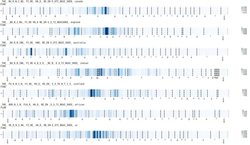
0.175
0.08
0.150
Avg Duration(s)
0.125
Frequency
0.06
0.100
0.04 0.075
0.02 0.050
0.025
0.00 0.000
aa
ae
ah
ao
aw
ay
b
ch
d
dh
eh
er
ey
f
g
hh
ih
iy
jh
k
l
m
n
ng
owv
oy
p
r
s
sh
sil
t
th
uh
uw
v
w
y
z
zh
aa
ae
ah
ao
aw
ay
b
ch
d
dh
eh
er
ey
f
g
hh
ih
iy
jh
k
l
m
n
ng
ow
oy
p
r
s
sh
t
th
uh
uw
v
w
y
z
zh
oo
Phones Phones
(a) Phonetic coverage histogram (b) Phonetic duration histogram
Figure 1: Phonetic coverage and duration histograms for the US accent. X-axis labels refer to individual phones.
we hope this work can serve as a starting point for very few speech samples overall, we chose tran-
further studies and spur more analysis-driven inves- scripts that had an utterance with the same text
tigations into end-to-end ASR models. The code spoken by a US-accented speaker. This finally led
used in our work is publicly available.1 to 3500 samples being chosen for each accent con-
taining text that appeared in at least two accents, at
2 Experimental Setup most six accents and 3.24 different accents on aver-
age. We chose the utterances to largely overlap in
In this section, we first introduce the dataset of
text so that differences in ASR performance could
accented speech samples used in our experiments,
be mostly attributed to acoustic differences and not
along with details of the phone-level alignments
language model-related differences.
that were necessary for our subsequent analyses.
We also provide a detailed description of the spe- Alignments: For our empirical investigation, we
cific end-to-end ASR model that we use in this require phone alignments for all the accented
work, along with important implementation details. speech samples. We used an existing Kaldi-based
forced aligner, gentle2 , to align the speech sam-
2.1 Dataset ples. The aligner uses the CMU dictionary and
We extracted accented speech samples from the accommodates multiple pronunciations for a word
Mozilla Common Voice speech corpus (Mozilla). which is important for accented speech. Although
The Voxforge corpus (Voxforge.org) was another the aligner was trained on US-accented speech, we
potential source for accented speech samples. How- found the alignments assigned to various accented
ever, we preferred the Mozilla corpus as the dataset speech samples to be fairly robust as determined by
is relatively cleaner, has larger diversity in speech a manual check of the alignments for a random set
across accents and more importantly contains the of Indian-accented utterances. The aligner failed to
same content rendered in different speech accents produce outputs on samples of poor quality; these
(which we exploited in our experimental analy- samples were omitted from our analysis.
sis). We considered accented speech samples from Figure 1(a) shows the coverage across phones for
seven different English accents: African, Aus- the US-accented speech samples and Figure 1(b)
tralian, Canadian, England, Indian, Scotland and shows the total duration of phones for US-accented
US. These were chosen to span the gamut of ac- speech samples. Phone coverage and phone dura-
cents in terms of how they differ from the primary tion distributions for all the other accents are almost
accent that was used to train the ASR system (US). identical in shape to the US accent. Aggregate plots
US and Canadian serve as native accents; African, visualizing these distributions across the remaining
Australian and England accents are sufficiently dif- accents are shown in Appendix A.
ferent from the native accents while Indian and
Scotland accents vary substantially. 2.2 End-to-end ASR: Deep Speech 2
We created a dataset of utterances in each ac- We chose DeepSpeech2 (Amodei et al., 2016) as
cent using the following heuristic. First, we chose our end-to-end ASR model. This is a widely-used
sentences that appeared in speech samples corre- architecture that directly maps speech features to
sponding to five or more accents (including US). graphemes and is trained using the Connectionist
For African and Scotland accents that contained Temporal Classification (CTC) loss (Graves et al.,
1 2
https://github.com/archiki/ Available at https://github.com/
ASR-Accent-Analysis/ lowerquality/gentle
3740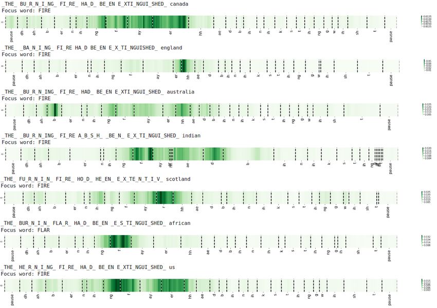
2006). The input to the model is a sequence of                             Utterances        Duration         Error
                                                                 Accent
frequency magnitude spectrograms (henceforth re-                           Train     Test   Train    Test   WER    CER
                                                                 African 2500        1000     3       1     28.7   16.2
ferred to as SPEC), obtained using a 20ms Ham-                   Australia 2500      1000     2       1     28.7   16.6
ming window and a stride of 10ms. With a                         Canada 2500         1000     2       1     18.7    9.9
sampling rate of 16kHz, we end up with 161-                      England 2500        1000     2       1     29.0   16.4
                                                                 Indian    2500      1000     2       1     49.1   31.6
dimensional input features. The first two layers                 Scotland 2500       1000     2       1     36.7   22.3
are 2D-convolutions with 32 kernels at each layer                US        2500      1000     3       1     20.4   10.9
with sizes 41 × 11 and 21 × 11, respectively. Both
convolutional layers have a stride of 2 in the fre-            Table 1: Data statistics of accented speech datasets. Du-
                                                               ration is approximated to hours and WER/CER refer to
quency domain while the first layer and second
                                                               the test error rates for each accent using DS2.
layer have a stride of 2 and 1, respectively, in
the time domain. This setting results in 1312 fea-
tures per time frame after the second convolutional            3     Gradient-based Analysis
layer which we will henceforth refer to as CONV.
                                                               Gradient-based techniques have been widely
The convolutional layers are followed by 5 bidi-
                                                               adopted as an explainability tool in both computer
rectional LSTMs (Hochreiter and Schmidhuber,
                                                               vision and NLP applications. In this section, we
1997), each with a hidden state size of 1024 dimen-
                                                               adapt some of these techniques to be used with
sions. These layers are henceforth referred to as
                                                               speech and derive insights based on how accents
RNN0 , RNN1 , RNN2 , RNN3 and RNN4 . The im-
                                                               modify gradient behavior.
plementation of this model is adapted from Naren
(2016). This model is trained on 960 hours of                  3.1    Attribution Analysis
US-accented speech obtained from the Librispeech
                                                               A simple gradient-based explanation method con-
corpus (Panayotov et al., 2015). All subsequent
                                                               siders the gradient of the output fj from a neural
experiments use this pretrained model, which we
                                                               network (where j denotes a target class) with re-
will refer to as DS2.
                                                               spect to an input xi (where i refers to the ith input
   Table 1 shows the performance of DS2 when
                                                               time-step used to index the input sequence x):
evaluated on speech samples from different accents.
Both word error rates (WER) and character error                                                      ∂fj
rates (CER) on the test sets are reported for each ac-                             grad(j, i, x) =
                                                                                                     ∂xi
cent. As expected, US and Canadian-accented sam-
ples perform best.3 DS2 has the most trouble rec-              Here, grad(j, i, x) serves as an approximate mea-
ognizing Indian-accented samples, incurring a high             sure of how much xi contributes to fj (Simonyan
WER of 49.1%, followed by Scotland-accented                    et al., 2014). For speech as input, xi would be
samples with a WER of 36.7%.                                   an acoustic feature vector (e.g. spectral features).
                                                               Thus, grad(j, i, x) would be a vector of element-
The next three sections are grouped based on the               wise gradients with respect to xi . For each xi , we
probing techniques we adopt to examine the effect              use the L2 norm to reduce the gradient vectors to
of accents on the internal representations learned             scalars: ai,j = kgrad(j, i, x)k2 . We refer to ai,j as
by the model:                                                  an attribution. We note here that instead of using
                                                               the L2 norm, one could use the dot product of the
   • Gradient-based analysis of the model (§3).                gradient grad(j, i, x) and the input xi as an alter-
                                                               nate gradient-based method (Denil et al., 2014).
   • Information-theoretic measures to directly                For our task, this attribution method seemed less
     quantify accent information in the learned rep-           suitable (compared to computing the L2 norm) as
     resentations (§4).                                        dot products would have the undesirable effect of
                                                               being sensitive to prosodic variations in speech and
   • Outputs of phone and accent classifiers at
                                                               speech sounds like fricatives or stop onsets which
     each layer (§5).
                                                               have sparse spectral distributions. (We refer in-
                                                               terested readers to Appendix C for visualizations
   3
     US-accented samples are drawn from various parts of the   using the dot product-based attribution method.)
US and are more diverse in accent, compared to the Canadian-
accented samples. We suspect this could be why US underper-       We compute character-level attribution from the
forms compared to Canada.                                      DS2 system using the following two-step approach.

                                                          3741
Figure 2: Example illustrating gradient attribution corresponding to the word “FIRE" across different accents.
First, we consider the output character with the for all the other accents.
highest softmax probability at each output time- To quantify the differences in alignment across
step. Next, we consider only non-blank characters accents suggested by the visualization in Figure 2,
produced as output and sum the gradients over all we measure the alignment accuracy using the earth
contiguous repetitions of a character (that would mover’s distance (EMD). For each accent, we com-
be reduced to a single character by the CTC algo- pute the EMD between two distributions, one de-
rithm)4 . Word-level attribution can be similarly rived from the attributions and the other from the
computed by summing the character-level attribu- reference phonetic alignment. The EMD between
tions corresponding to each character that makes two distributions p and q over the set of frames (or
up the word. rather, frame sequence numbers) T is defined as
Figure 2 illustrates how attribution changes for a X
EMD(p, q) = inf |i − j| · Z(i, j)
specific word, “FIRE", across different accents. We Z
i,j∈T
consider speech samples from all seven accents cor-
responding to the same underlying reference text, where the infimum is over all “transportation
P func-
“The burning fire had been extinguished". Each sub- tions” Z : T × T →PR+ such that j∈T Z(i, j) =
plot also shows the phonetic alignment of the text p(i) (for all i) and i∈T Z(i, j) = q(j) (for all j).
on its x-axis. We observe that the attributions for
“FIRE" are fairly well-aligned with the underlying Given a correctly predicted word, we define the
speech in the US and Canadian samples; the attri- distribution p as the uniform distribution over the
butions appear to deviate more in their alignments frames that are aligned with the word, and q as the
distribution obtained by normalizing the word-level
4
The CTC algorithm produces output probabilities for ob- attribution of the word in the utterance. For each
serving a “blank”, signifying no label. Excluding the blank accent, we sample a set of words that were cor-
symbol from our analysis helped with reducing gradient com-
putation time. We also confirmed that including the blank rectly predicted (equally many for all accents) and
symbol did not change the results from our analysis. compute the average of the EMD between the dis-
3742EMD TIMIT
Accent 0.8 canada
C0 C1 C2 Overall us
england
US 43.54 42.42 39.55 42.6 australia
Phone Focus
0.6
scotland
Canada 42.17 39.68 40.47 40.94 african
Indian 53.07 47.47 49.63 50.34 0.4 indian
African 46.63 42.61 41.05 44.3
0.2
England 47.0 41.52 43.44 44.3
Scotland 45.34 41.38 41.65 43.26
0.0 CONV RNN_0 RNN_1 RNN_2 RNN_3 RNN_4
Australian 46.91 44.24 47.45 45.87 Layers
Table 2: EMD trends quantifying the difference in at- Figure 3: Comparison of phone focus across layers for
tributions across accents. C0 , C1 and C2 are clusters various accents.
of words containing {1-2}, 3 and {4-5} phones, respec-
tively
climbs through the layers. But somewhat surpris-
tributions p and q corresponding to each word. This ingly, we find that there is little variation of these
average serves as an alignment accuracy measure trends across accents. This suggests that informa-
for the accent. For the EMD analysis, we restrict tion mixing is largely dictated by the network itself,
ourselves to a set of 380 sentences that have cor- rather than by the details of the data.
responding speech utterances in all accents. This The quantities we use to measure information
way, the content is mostly identical across all ac- mixing are inspired by Brunner et al. (2020). We
cents. Table 2 shows the averaged EMD values define the contribution of the ith input frame xi to
for each accent computed across all correctly pre- the final output of the network f via the representa-
dicted words. Larger EMD values signify poorer tion elj in a given layer l corresponding to frame j
alignments. The overall values clearly show that as:
d l
∂ej (k)
the alignments from US and Canadian-accented l
X ∂f
ĝi,j = (1)
samples are most accurate and the alignments from ∂elj (k)
k=1
∂xi 2
the Indian-accented samples are most inaccurate. where elj is a d-dimensional vector (elj (k) refers
We also cluster the words based on the number of to the k th dimension of elj ), and f consists of the
phones in each word, with C0 , C1 and C2 referring non-blank characters in the maximum probability
to words with {1-2}, 3 and {4-5} phones, respec- output (after the softmax layer). We use a normal-
tively. As expected, words in C0 , being smallest in l to compare the contribution to
ized version of ĝi,j
size, deviate most from the reference distribution l
ej from different xi :
and incur larger EMD values (compared to C1 and l
l
ĝi,j
C2 ). The overall trend across accents remains the gi,j = PT
l
same for each cluster. n=1 ĝn,j
For this analysis, we used a subset of 250 utter-
3.2 Information Mixing Analysis ances for each accent that have almost the same
Another gradient-based analysis we carried out is underlying content.5
to check if accents affected how, at various levels, A measure of “focus” of an input phone at level
the representation at each frame is influenced by l – how much the frames at level l corresponding
the signal at the corresponding input frame. One to that phone draw their contributions from the
can expect that, in layers higher up, the represen- corresponding frames in the input – is obtained
by summing up gi,j l over i, j corresponding to the
tation at each frame mixes information from more
and more input frames. However, it is reasonable phone. Figure 3 shows this quantity, averaged over
to expect that most of the contribution to the rep- all phones in all the utterances for each accent. We
resentation should still come from the frames in observe that the focus decreases as we move from
a window corresponding to the same phone. (We CONV to RNN4 , with the largest drop appearing
examine the contribution of neighboring phones in between CONV and RNN0 . This is intuitive as we
Appendix B) expect some of the focus to shift from individual
As detailed below, we devise quantities that mea-
5
sure the extent of information mixing and apply This smaller sample was chosen for faster gradient com-
putations and gave layer-wise phone accuracies similar to what
them to our systems. Not surprisingly, as shown we obtained for the complete test set of 1000 utterances. A
below, we do observe that mixing increases as one plot showing these consistent trends is included in Appendix D
37430.75 TIMIT 0.35 1000 Clusters
Binary Focus Measure 0.70 canada 5000 Clusters
us 0.30 10000 Clusters
0.65
england 0.25
0.60 australia
0.55 scotland 0.20
MI
0.50 african
indian 0.15
0.45
0.10
0.40
0.35 0.05
CONV RNN_0 RNN_1 RNN_2 RNN_3 RNN_4 SPEC CONV RNN_0 RNN_1 RNN_2 RNN_3 RNN_4
Layers Layers
Figure 4: Variation in binary focus measure, averaged Figure 5: Mutual Information between hidden represen-
over all the phones, across layers for various accents. tations and accents across layers.
phones to their surrounding context, as we move much information about accents is encoded within
to a recurrent layer (from the CONV layer). This the representations at each layer. Towards this, mo-
trend persists in moving from RNN0 to RNN4 tivated by Voita et al. (2019), we compute the mu-
with the focus on individual phones steadily drop- tual information (MI) between random variables elx
ping. We also see a consistent albeit marginal trend and α, where elx refers to a representation at layer l
across accents with US/Canadian-accented samples corresponding to input x and α ∈ [0, 6] is a discrete
showing the lowest focus. random variable signifying accents. We define a
For each input phone, one can also define a bi- probability distribution for elx by discretizing the
nary measure of focus at level l, which checks that space of embeddings via k-means clustering (Saj-
the focus of the frames at that level has not shifted jadi et al., 2018). We use mini-batched k-means to
to an input phone other than the one whose frames cluster all the representations corresponding to files
it corresponds to. That is, this binary focus measure in the test sets mentioned in Table 1 across accents
is 1 if the focus of the phone at a level as defined and use the cluster labels thereafter to compute MI.
above is larger than the contribution from the input
frames of every other phone. Figure 4 shows how Figure 5 shows how MI varies across different
this measure, averaged across all phones for each layers for three different values of k. Increasing
accent, varies across layers. Again, we see that fo- k would naturally result in larger MI values. (The
cus is highest in the first CONV layer, dropping to maximum possible value of MI for this task would
70% at RNN1 and 45% at RNN3 . Further, again, be log2 (7).) We observe a dip in MI going from
we observe very similar trends across all accents. spectral features SPEC to CONV, which is natu-
From both the above analyses of focus, we ob- ral considering that unprocessed acoustic features
serve that there is a pronounced drop in focus would contain most information about the under-
through the layers, but this trend is largely indepen- lying accent. Interestingly, we observe a rise in
dent of the accent. We also plot variations for the MI going from CONV to RNN0 signifying that
well-known TIMIT database (Garofolo, 1993) in the first layer of RNN-based representations carries
both Figures 3 and 4 to confirm that the same trend the most information about accent (not considering
persists. For TIMIT, we used the samples from the acoustic features). All subsequent RNN layers
the specified test set along with the phonetic align- yield lower MI values.
ments that come with the dataset. We conclude that
Apart from the MI between representations and
information mixing, and in particular, the measures
accents that capture how much accent information
of focus we used, are more a feature of the network
is encoded within the hidden representations, we
than the data.
also compute MI between representations and a
4 Information-Theoretic Analysis discrete random variable signifying phones. The
MI computation is analogous to what we did for
In the previous section, we used gradient-based accents. We will now have a separate MI plot
methods to examine how much an input frame (or across layers corresponding to each accent. Fig-
a set of frames corresponding to a phone or a word) ure 6 shows the MI values across layers for each
contributes to the output and how these measures accent when k = 500 and k = 2000. We see
change with varying accents. Without computing an overall trend of increasing MI from initial to
gradients, one could also directly measure how later layers. Interestingly, the MI values across ac-
3744us canada indian scotland england australia african
3.0
2.5
MI
2.0
(a) US accent
1.5
1.0
SPEC CONV RNN_0 RNN_1 RNN_2 RNN_3 RNN_4
Layers
(a) Cluster Size: 500
(b) Indian accent
us canada indian scotland england australia african
3.5 Figure 7: t-SNE plot for representations of top 10
3.0 phones across US and Indian-accented samples, with
the following layers on the X-axis (from left to right):
MI
2.5
SPEC, CONV, RNN0 , RNN1 , RNN2 , RNN3 , RNN4
2.0
˙
1.5
SPEC CONV RNN_0 RNN_1 RNN_2 RNN_3 RNN_4
Layers
(b) Cluster Size: 2000
malization (Ioffe and Szegedy, 2015) followed by
ReLU activations for each unit. The network also
Figure 6: Mutual Information between representations contained two max-pooling layers of size (5,3) and
and phones for different clusters sizes and accents. (3,2), respectively, and a final linear layer with hid-
den dimensionality of 500 (with a dropout rate of
0.4). Table 1 lists the number of utterances we
cents at RNN4 exhibit a familiar ordering where used for each accent for training and evaluation.
US/Canadian accents receive the highest MI value The accent classifiers were trained for 25 epochs
while Indian and Scotland’s accents receive the using Adam optimizer (Kingma and Ba, 2015) and
lowest MI value. a learning rate of 0.001.
We also attempt to visualize the learned phone Figure 8 shows the accent accuracies obtained
representations by projecting down to 2D. For a by the accent classifier specific to each layer (along
specific phone, we use the precomputed alignments with error bars computed over five different runs).
to compute averaged layer-wise representations RNN0 is most accurate with an accuracy of about
across the frames within each phone alignment. 33% and RNN4 is least accurate. It is interesting
Figure 7 shows t-SNE based (Maaten and Hinton, that RNN0 representations are most discriminative
2008) 2D visualizations of representations for the across accents; this is also consistent with what we
10 most frequent phones in our data, {‘ah’, ‘ih’, observe in the MI plots in Figure 5.
‘iy’, ‘dh’, ‘d’, ‘l’, ‘n’, ‘r’, ‘s’, ‘t’}. Each subplot
corresponds to a layer in the network. The plots 5.2 Phone Classifiers
for phones from the US-accented samples appear
Akin to accent classifiers, we build a phone classi-
to have slightly more well-formed clusters, com-
fier for each layer whose input representations are
pared to the Indian-accented samples. These kinds
labeled using phone alignments. We train a simple
of visualizations of representations are, however,
multi-layer perceptron for each DS2 layer (500-
limiting and thus motivates the need for analysis
dimensional, dropout rate of 0.4) for 10 epochs
like the MI computation presented earlier.
5 Classifier-driven Analysis 35
30
5.1 Accent Classifiers
Accuracy %
25
20
We train an accent classifier for each layer that
15
takes the corresponding representations from the
10
layer as its input. We implemented a classifier with SPEC CONV RNN_0 RNN_1
Layers
RNN_2 RNN_3 RNN_4
two convolutional layers of kernel size, stride and
padding set to (31,21), (3,2), (15,10) and (11,5), Figure 8: Accuracy (%) of accent probes trained on
(2,1) and (5,2), respectively. We used batch nor- hidden representations at different layers.
374590
sures in the information mixing analysis are new.
80
We also highlight that this is the first instance of
analysis of ASR consisting of multiple analysis
70 techniques. On the one hand, this has uncovered
robust trends that manifest in more than one anal-
60
ysis. On the other hand, it also shows how some
Accuracy %
avg us
50
avg canada
avg indian
trends are influenced more by the neural-network
avg scotland
avg england architecture more than the data. This provides a
avg australia
40 avg african
TIMIT
platform for future work in speech neural-network
us analysis, across architectures, data-sets and tasks.
canada
30 indian
scotland In our results, we encountered some unexpected
england
australia
african
details. For instance, while the RNN0 layer is
20
SPEC CONV RNN_0 RNN_1
Layers
RNN_2 RNN_3 RNN_4 seen to reduce the phone focus the most, uniformly
across all accents (as shown in Figure 3, it is also
Figure 9: Trends in accuracy (%) of phone probes seen to segregate accent information the most, re-
for frame-level (dotted) and averaged representations covering accent information “lost” in the convo-
(solid) at different layers.
lution layer (as shown in Figure 5). We also see
this trend surfacing in Figure 8 where the accent
using the Adam optimizer. We train both frame- classifier gives the highest accuracy for RNN0 and
level classifiers, as well as phone-level classifiers the accuracies quickly taper off for subsequent lay-
that use averaged representations for each phone ers. This suggests that the first RNN layer is most
as input. The accuracies of both types of phone discriminative of accents. Models that use an ad-
classifiers are shown in Figure 9. As expected, versarial objective to force the representations to be
the phone accuracies improve going from SPEC to accent invariant (e.g., (Sun et al., 2018)) might ben-
RNN4 and the accuracies of US/Canadian samples efit from defining the adversarial loss as a function
are much higher than that of Indian samples. Clas- of the representations in the first RNN layer.
sifiers using the averaged representations consis-
tently perform much better than their frame-level 7 Related Work
counterparts. We note that Belinkov and Glass 7.1 Accented Speech Recognition
(2017) report a dip in phone accuracies for the last
Huang et al. (2001) show that accents are the pri-
RNN layers, which we do not observe in our exper-
mary source of speaker variability. This poses a
iments. To resolve this inconsistency, we ran phone
real-world challenge to ASR models which are pri-
classifiers on TIMIT (which was used in Belinkov
marily trained on native accented datasets. The
and Glass (2017)) using representations from our
effect of accents is not limited to the English lan-
DS2 model and the dip in RNN4 accuracies sur-
guage, but also abundant in other languages such
faced (as shown in Figure 9). This points to differ-
as Mandarin, Spanish, etc.
ences between the TIMIT and Mozilla Common
Voice datasets. (An additional experiment exam- An interesting line of work exploits the abil-
ining how phone classifiers behave on different ity to identify accents in order to improve perfor-
datasets is detailed in Appendix D.) mance. Zheng et al. (2005) combine accent detec-
tion, accent discriminative acoustic features, acous-
6 Discussion tic model adaptation using MAP/MLLR and model
selection to achieve improvements over accented
This is the first detailed investigation of how accent Mandarin speech.Vergyri et al. (2010) investigate
information is reflected in the internal representa- the effect of multiple accents on the performance
tions of an end-to-end ASR system. In devising of an English broadcast news recognition system
analysis techniques for ASR, while we do follow using a multiple accented English dataset. They
the broad approaches in the literature, the details report improvements by including data from all
are often different. Most notably, the use of EMD accents for an accent-independent acoustic model
for attribution analysis is novel, and could be of training.
interest to others working with speech and other Sun et al. (2018) propose the use of domain ad-
temporal data. Similarly, the phone focus mea- versarial training (DAT) with a Time Delay Neu-
3746ral Network (TDNN)-based acoustic model. They used to analyze images, Li et al. (2020) propose
use native speech as the source domain and ac- reconstructing speech from the hidden representa-
cented speech as the target domain, with the goal tions at each layer using highway networks. Apart
of generating accent-invariant features which can from ASR, analysis techniques have also been used
be used for recognition. Jain et al. (2018) also use with speaker embeddings for the task of speaker
an accent classifier in conjunction with a multi- recognition (Wang et al., 2017).
accent TDNN based acoustic model in a multi- The predominant tool of choice for analyzing
task learning (MTL) framework. Further, Viglino ASR models in prior work has been classifiers
et al. (2019) extended the MTL framework to use that are trained to predict various phonological at-
an end-to-end model based on the DS2 architec- tributes using quantities extracted from the model
ture and added a secondary accent classifier that as its input. We propose a number of alternatives
uses representations from intermediate recurrent other than just the use of classifiers to probe for
layers as input. Chen et al. (2020) propose an al- information within an end-to-end ASR model. We
ternate approach using generative adversarial net- hope this spurs more analysis-driven investigations
works (GANs) to disentangle accent-specific and into end-to-end ASR models.
accent-invariant components from the acoustic fea-
tures. 8 Summary
This work presents a thorough analysis of how ac-
7.2 Analysis of ASR Models cent information manifests within an end-to-end
Nagamine et al. (2015, 2016) were the first to ex- ASR system. The insights we gleaned from this
amine representations of a DNN-based acoustic investigation provide hints on how we could po-
model trained to predict phones. They computed tentially adapt such end-to-end ASR models, using
selectivity metrics for each phoneme and found auxiliary losses, to be robust to variations across
better selectivity and more significance in deeper accents. We will investigate this direction in future
layers. This analysis was, however, restricted to work.
the acoustic model. Belinkov and Glass (2017)
were the first to analyze a Deep Speech 2 model Acknowledgements
by training phone classifiers that used representa- The authors thank the anonymous reviewers for
tions at each layer as its input. These ideas were their constructive feedback and comments. The sec-
further extended in Belinkov et al. (2019) with clas- ond author gratefully acknowledges support from
sifiers used to predict phonemes, graphemes and a Google Faculty Research Award and IBM Re-
articulatory features such as place and manner of search, India (specifically the IBM AI Horizon
articulation. Belinkov and Glass (2019) present Networks-IIT Bombay initiative).
a comparison of different analysis methods that
have been used in prior work for speech and lan-
guage. The methods include recording activations References
of pretrained networks on linguistically annotated
Afra Alishahi, Marie Barking, and Grzegorz Chru-
datasets, using probing classifiers, analyzing atten- pała. 2017. Encoding of phonology in a recurrent
tion weights and ABX discrimination tasks (Schatz neural model of grounded speech. In Proceedings
et al., 2013). of the 21st Conference on Computational Natural
Language Learning (CoNLL 2017), pages 368–378.
Other related work includes the analysis of an
audio-visual model for recognition in Alishahi et al. Dario Amodei, Sundaram Ananthanarayanan, Rishita
(2017), where the authors analyzed the activations Anubhai, Jingliang Bai, Eric Battenberg, Carl Case,
of hidden layers for phonological information and Jared Casper, Bryan Catanzaro, Qiang Cheng, Guo-
liang Chen, et al. 2016. Deep Speech 2: End-to-End
observed a hierarchical clustering of the activations. Speech Recognition in English and Mandarin. In
Elloumi et al. (2018) use auxiliary classifiers to pre- Proceedings of the 33rd International Conference on
dict the underlying style of speech as being sponta- Machine Learning, pages 173–182.
neous or non-spontaneous and as having a native
Yonatan Belinkov, Ahmed Ali, and James Glass. 2019.
or non-native accent; their main task was to pre- Analyzing Phonetic and Graphemic Representations
dict the performance of an ASR system on unseen in End-to-End Automatic Speech Recognition. In
broadcast programs. Analogous to saliency maps Proc. Interspeech 2019, pages 81–85.
3747Yonatan Belinkov and James Glass. 2017. Analyz- Chao Huang, Tao Chen, Stan Li, Eric Chang, and
ing Hidden Representations in End-to-End Auto- Jianlai Zhou. 2001. Analysis of speaker variabil-
matic Speech Recognition Systems. In Advances ity. In Seventh European Conference on Speech
in Neural Information Processing Systems, pages Communication and Technology, pages 1377–1380.
2441–2451.
Sergey Ioffe and Christian Szegedy. 2015. Batch nor-
Yonatan Belinkov and James Glass. 2019. Analysis malization: Accelerating deep network training by
Methods in Neural Language Processing: A Survey. reducing internal covariate shift. In Proceedings of
Transactions of the Association for Computational the 32nd International Conference on International
Linguistics, pages 49–72. Conference on Machine Learning, pages 448–456.
Gino Brunner, Yang Liu, Damián Pascual, Oliver Abhinav Jain, Minali Upreti, and Preethi Jyothi. 2018.
Richter, Massimiliano Ciaramita, and Roger Wat- Improved Accented Speech Recognition Using Ac-
tenhofer. 2020. On Identifiability in Transform- cent Embeddings and Multi-task Learning. In Proc.
ers. In International Conference on Learning Interspeech 2018, pages 2454–2458.
Representations.
Diederik P Kingma and Jimmy Ba. 2015. Adam: A
Yi-Chen Chen, Zhaojun Yang, Ching-Feng Yeh, Ma- method for stochastic optimization. In International
haveer Jain, and Michael L Seltzer. 2020. AIP- Conference on Learning Representations (ICLR).
Net: Generative Adversarial Pre-training of Accent-
invariant Networks for End-to-end Speech Recogni- Chung-Yi Li, Pei-Chieh Yuan, and Hung-Yi Lee. 2020.
tion. In ICASSP 2020 - 2020 IEEE International What Does a Network Layer Hear? Analyzing Hid-
Conference on Acoustics, Speech and Signal den Representations of End-to-End ASR Through
Processing (ICASSP), pages 6979–6983. Speech Synthesis. In ICASSP 2020 - 2020 IEEE
International Conference on Acoustics, Speech and
Chung-Cheng Chiu, Tara N Sainath, Yonghui Wu, Ro- Signal Processing (ICASSP), pages 6434–6438.
hit Prabhavalkar, Patrick Nguyen, Zhifeng Chen,
Anjuli Kannan, Ron J Weiss, Kanishka Rao, Eka- Laurens van der Maaten and Geoffrey Hinton. 2008.
terina Gonina, et al. 2018. State-of-the-Art Speech Visualizing data using t-SNE. Journal of machine
Recognition with Sequence-to-Sequence Models. In learning research, 9:2579–2605.
2018 IEEE International Conference on Acoustics, Mozilla. Mozilla common voice dataset. https://
Speech and Signal Processing (ICASSP), pages voice.mozilla.org/en/datasets.
4774–4778.
Tasha Nagamine, Michael L Seltzer, and Nima
Misha Denil, Alban Demiraj, and Nando De Freitas. Mesgarani. 2015. Exploring How Deep Neural
2014. Extraction of Salient Sentences from Labelled Networks Form Phonemic Categories. In Proc.
Documents. arXiv preprint arXiv:1412.6815. Interspeech 2015, pages 1912–1916.
Zied Elloumi, Laurent Besacier, Olivier Galibert, and Tasha Nagamine, Michael L Seltzer, and Nima Mes-
Benjamin Lecouteux. 2018. Analyzing Learned garani. 2016. On the Role of Nonlinear Transforma-
Representations of a Deep ASR Performance Pre- tions in Deep Neural Network Acoustic Models. In
diction Model. In Proceedings of the 2018 Proc. Interspeech 2016, pages 803–807.
EMNLP Workshop BlackboxNLP: Analyzing and
Interpreting Neural Networks for NLP, pages 9–15. Sean Naren. 2016. https://github.com/
SeanNaren/deepspeech.pytorch.git.
John S Garofolo. 1993. Timit acoustic phonetic con-
tinuous speech corpus. Linguistic Data Consortium, Vassil Panayotov, Guoguo Chen, Daniel Povey, and
1993. Sanjeev Khudanpur. 2015. Librispeech: an ASR
corpus based on public domain audio books. In
Alex Graves, Santiago Fernández, Faustino Gomez, 2015 IEEE International Conference on Acoustics,
and Jürgen Schmidhuber. 2006. Connectionist Tem- Speech and Signal Processing (ICASSP), pages
poral Classification: Labelling Unsegmented Se- 5206–5210.
quence Data with Recurrent Neural Networks. In
Proceedings of the 23rd International Conference on Mehdi SM Sajjadi, Olivier Bachem, Mario Lucic,
Machine Learning, pages 369–376. Olivier Bousquet, and Sylvain Gelly. 2018. As-
sessing Generative Models via Precision and Re-
Sepp Hochreiter and Jürgen Schmidhuber. 1997. call. In Advances in Neural Information Processing
Long Short-Term Memory. Neural computation, Systems, pages 5228–5237.
9(8):1735–1780.
Thomas Schatz, Vijayaditya Peddinti, Francis Bach,
Takaaki Hori, Shinji Watanabe, Yu Zhang, and William Aren Jansen, Hynek Hermansky, and Emmanuel
Chan. 2017. Advances in joint CTC-attention based Dupoux. 2013. Evaluating speech features with
end-to-end speech recognition with a deep CNN en- the Minimal-Pair ABX task: Analysis of the clas-
coder and RNN-LM. In Proc. Interspeech 2017, sical MFC/PLP pipeline. In Proc. Interspeech 2013,
pages 949–953. pages 1–5.
3748Karen Simonyan, Andrea Vedaldi, and Andrew Zis-
serman. 2014. Deep Inside Convolutional Net-
works: Visualising Image Classification Models and
Saliency Maps. In International Conference on
Learning Representations, ICLR, Workshop Track
Proceedings.
Sining Sun, Ching-Feng Yeh, Mei-Yuh Hwang, Mari
Ostendorf, and Lei Xie. 2018. Domain adversar-
ial training for accented speech recognition. In
2018 IEEE International Conference on Acoustics,
Speech and Signal Processing (ICASSP), pages
4854–4858.
Dimitra Vergyri, Lori Lamel, and Jean-Luc Gauvain.
2010. Automatic Speech Recognition of Multiple
Accented English Data. In Proc. Interspeech 2010,
pages 1652–1655.
Thibault Viglino, Petr Motlicek, and Milos Cernak.
2019. End-to-end Accented Speech Recognition.
Proc. Interspeech 2019, pages 2140–2144.
Elena Voita, Rico Sennrich, and Ivan Titov. 2019.
The bottom-up evolution of representations in the
transformer: A study with machine translation and
language modeling objectives. In Conference on
Empirical Methods in Natural Language Processing
(EMNLP), pages 4396–4406.
Voxforge.org. Free and open source speech recognition
(linux, windows and mac) - voxforge.org. http://
www.voxforge.org/. Accessed 06/25/2014.
Shuai Wang, Yanmin Qian, and Kai Yu. 2017. What
does the speaker embedding encode? In Proc.
Interspeech 2017, pages 1497–1501.
Yanli Zheng, Richard Sproat, Liang Gu, Izhak Shafran,
Haolang Zhou, Yi Su, Daniel Jurafsky, Rebecca
Starr, and Su-Youn Yoon. 2005. Accent detection
and speech recognition for shanghai-accented man-
darin. In Ninth European Conference on Speech
Communication and Technology, pages 217–220.
3749Appendix 0.6 CONV
RNN_0
0.5 RNN_1
RNN_2
0.4
A Dataset Information across Accents RNN_3
Focus
0.3 RNN_4
0.2
Figure 10(a) shows the frequency of each phone 0.1
across all the accents used in our dataset. Fig- 0.0
Actual 1st 2nd 3rd 4th5th 6th8th 9th11th 12thonwards
Neighbours
ure 10(b) shows the average duration in seconds
of each phone across all the accents in our dataset. Figure 11: Phone focus of the aligned (actual) phone
The error bars for each phone denote the variance as compared to its preceding and succeeding neighbors
in coverage and duration across all the accents. We on the TIMIT dataset.
observe that the variance is very small, thus indi-
cating that the difference in phone coverage and
dataset. We found the trends from such a com-
duration across accents is minimal.
parison of phone focus across neighbors on our
accented datasets to be very similar to the trends
0.08 exhibited by the different layers on TIMIT.
Frequency
0.06
0.04
C Experiments on Attribution Analysis
0.02 Common gradient-based explainability techniques
0.00 include examining the gradient, as well as the dot
aa
ahe
awo
ay
b
ch
d
dh
eh
er
ey
f
g
hh
ih
iy
jh
k
l
m
n
ng
oov
ow
oy
p
r
s
sh
sil
t
th
uh
uw
v
w
y
z
zh
a
a
Phones product of the gradient and the input. We analyze
(a) Phonetic coverage histogram both these techniques in this section. We also com-
pare grapheme-level attributions with word-level
0.200
0.175
attributions.
0.150 In Figure 12, we visualize grapheme-level at-
Avg Duration(s)
0.125 tributions for the text “I’m going to them". The
0.100
0.075 grapheme-level attribution is shown for the first
0.050 letter in the transcription. The blue heatmaps corre-
0.025
0.000
spond to computing the absolute value of the dot
product of the gradient and the input (referred to
aa
ae
ah
awo
ay
b
ch
d
dh
eh
er
ey
f
g
hh
ih
iy
jh
k
l
m
n
ng
ow
oy
p
r
s
sh
t
th
uwh
v
w
y
z
zh
a
u
Phones
as INP-GRAD)6 and the green heatmaps corre-
(b) Phonetic duration histogram
spond to computing the L2 norm of the gradient
(referred to as GRAD). On comparing the two, we
Figure 10: Histograms showing phonetic coverage and
duration for all accents with labels on the X-axis show- observe that the former is more diffuse and dis-
ing phones. continuous than the latter. In general, we observe
that the grapheme-level attributions are distributed
non-uniformly across the frames of the underlying
B Information Mixing: Neighbourhood phone. For some accents, the attribution of the
Analysis frames of the nearby phones is also comparable.
Figure 13 shows the word-level attributions for
We explore the variation in the phone focus mea- the word “FIRE" using INP-GRAD. This can be
sure described in Section 3.2 for the aligned phone contrasted with the word-level attributions for the
and its neighbors that precede and succeed it, same word shown in Figure 2 in Section 3.1. There
across different layers of the model. Figure 11 is more discontinuity in INP-GRAD compared to
shows that the focus of the actual (input) phone GRAD; this could be attributed to the underlying
is maximum for the CONV layer and shows the speech containing sparse spectral distributions near
fastest decrease across neighbors. This is expected fricatives or stop onsets, thus making alignments
due to the localized nature of convolutions. From from the former technique less reliable for further
RNN0 to RNN4 the focus of the actual phone de- downstream processing.
creases and is increasingly comparable to the first
6
(and other) neighbors. We see an increase in neigh- Unlike tasks like sentiment analysis where the positive
and negative signs of the dot product carry meaningful infor-
bors 12th and onwards because of its cumulative mation, in our setting we make use of the absolute value of
nature. Figure 11 shows this analysis for the TIMIT the dot product.
3750Figure 12: Grapheme-level attributions for the first letter in the text transcribed by the model.
D Phone Classifiers speech samples from Mozilla Common Voice for
all layers (except RNN3 and RNN4 ). This reflects
D.1 Effect of Changing Distribution of the differences in both datasets; TIMIT comprises
Phones clean broadband recordings while the speech sam-
ples from Common Voice are much noisier.
We investigate the influence of changing the distri-
bution of phones on phone classifier accuracies. We
sample phones from the Mozilla Common Voice D.2 Effect of Changing Sample Size
dataset so as to mimic the phone distribution of
the TIMIT dataset. Figure 14 shows no significant In Section 3.2, we subsample 250 utterances from
difference in changing the phone distribution. The 1000 in the original test set. Even with only 250
plot also shows the accuracy on the TIMIT dataset utterances, we find the phone accuracy trends to be
which is higher than the phone accuracies for the preserved as shown in Figure 15.
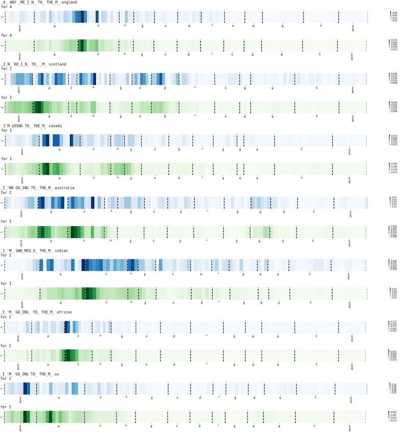
3751Figure 13: Word-level attributions for the word corresponding to “FIRE” in the transcription by the model.
70
70
60 60
us 250 us
Accuracy %
Accuracy %
canada 250 canada
50 50
indian 250 indian
scotland 250 scotland
england 250 england
australia 250 australia
40 african 40 250 african
TIMIT us
us TIMIT distr canada
canada TIMIT distr indian
30 indian TIMIT distr 30 scotland
scotland TIMIT distr
african TIMIT distr england
australia TIMIT distr australia
20 england TIMIT distr african
20
SPEC CONV RNN_0 RNN_1 RNN_2 RNN_3 RNN_4 SPEC CONV RNN_0 RNN_1 RNN_2 RNN_3 RNN_4
Layers Layers
Figure 14: Trends in phone accuracy on Common Figure 15: Trends in phone accuracy for 250 utterances
Voice accented speech samples using TIMIT’s phone (solid) randomly sampled from our test set consisting
distribution (dotted) and the original phone distribution of 1000 utterances (dashed) for each accent.
(solid). The line in black shows performance on the
TIMIT dataset.
and Scotland, indicating that for the latter even at
the final layers there is some residual confusion
D.3 Confusion in Phones remaining. Instead of showing all the confusion
We analyze the confusion in the phones for each ac- matrices for each accent, we resort to an aggregate
cent7 . As expected, phone confusions for each ac- entropy-based analysis. In Figure 16, we compute
cent are more prevalent in initial layers compared to the entropy of the phone distributions, averaged
the later layers. A comparison between the confu- over all phones, across layers for different accents.
sion matrices at layer RNN4 for all accents shows We observe that in the beginning the accents are
a prominent difference between native accents, like clustered together and they diverge gradually as we
US and Canada, and non-native accents, like Indian move to higher layers. As we approach the last 3
7
recurrent layers (RNN2 , RNN3 and RNN4 ), we
Available at https://github.com/archiki/
ASR-Accent-Analysis/tree/master/ find a clear separation, with Indian followed by
PhoneProbes Scotland accent having the highest entropy while
3752Top-5 Confusions
Accent
1st 2nd 3rd 4th 5th
US aa-ao (0.134) zh-jh (0.125) z-s (0.112) aa-ah (0.109) g-k (0.092)
Canada zh-ah (0.118) zh-v (0.088) g-k (0.074) th-t (0.072) y-uw (0.070)
African z-s (0.102) ae-ah (0.098) er-ah (0.098) aa-ah (0.089) g-k (0.086)
Australia zh-sh (0.462) th-t (0.115) aa-ah (0.105) g-k (0.097) z-s (0.92)
England zh-sh (0.222) z-s (0.126) aa-ah (0.121) ae-ah (0.119) th-t (0.114)
Scotland jh-d (0.148) ch-t (0.146) zh-sh (0.125) zh-ey (0.125) ae-ah (0.123)
Indian zh-ah (0.38) th-t (0.262) z-s (0.175) uh-uw (0.154) er-ah (0.153)
Table 3: Five highest confusion pairs for all accents. Notation: phonei -phonej (x) means that phonei is confused
with phonej with likelihood x.
US and Canada samples have the lowest entropy.
us canada indian scotland england australia african
0.060
0.055
Average Entropy
0.050
0.045
0.040
0.035
SPEC CONV RNN_0 RNN_1 RNN_2 RNN_3 RNN_4
Layers
Figure 16: Entropy of the distribution of the outputs of
the phone probes averaged across phones and plotted
for each accent across layers.
Table 3 shows the five highest confusion pairs for
each accent. We observe that each accent displays a
different trend and most confusions make phonetic
sense; for example, z getting confused as s, or g
getting confused as k.
3753You can also read