Hybrid deep convolutional neural network with one-versus-one approach for solar flare prediction
←
→
Page content transcription
If your browser does not render page correctly, please read the page content below
MNRAS 507, 3519–3539 (2021)                                                                                         https://doi.org/10.1093/mnras/stab2132
Advance Access publication 2021 July 26

Hybrid deep convolutional neural network with one-versus-one approach
for solar flare prediction
Yanfang Zheng, Xuebao Li,‹ Yingzhen Si, Weishu Qin and Huifeng Tian
School of computer science, Jiangsu University of Science and Technology, Zhenjiang, China

Accepted 2021 July 19. Received 2021 July 1; in original form 2021 February 8

                                                                                                                                                             Downloaded from https://academic.oup.com/mnras/article/507/3/3519/6328501 by guest on 07 December 2021
ABSTRACT
We propose a novel hybrid Convolutional Neural Network (CNN) model with one-versus-one approach to forecast solar flare
occurrence with the outputs of four classes (No-flare, C, M, and X) within 24 h. We train and test our model using the same
data sets as in Zheng, Li & Wang, and then compare our results with previous models using the true skill statistic (TSS) as
primary metric. The main results are as follows. (1) This is the first time that the CNN model in conjunction with one-versus-one
approach is used in solar physics to make multiclass flare prediction. (2) In the four-class flare prediction, our model achieves
quite high mean scores of TSS = 0.703, 0.489, 0.432, and 0.436 for No-flare, C, M, and X class, respectively, which are
much better than or comparable to those of previous studies. In addition, our model obtains TSS scores of 0.703 ± 0.070 for
≥C-class and 0.739 ± 0.109 for ≥M-class predictions. (3) This is the first attempt to open the black-box CNN model to study
the visualization of feature maps for interpreting the prediction model. Furthermore, the visualization results indicate that our
model pays attention to the regions with strong gradient, strong intensity, high total intensity, and large range of the intensity
in high-level feature maps. The median gradient and intensity, the total intensity, and the range of the intensity for high-level
feature maps increase approximately with the increase of flare level.
Key words: magnetic fields – methods: data analysis – techniques: image processing – Sun: activity – Sun: flares.

                                                                                automatically acquiring features from image data without human
1 I N T RO D U C T I O N
                                                                                intervention. There are a few attempts to apply CNNs to forecast
Solar flares could cause space weather hazards in the near-Earth                solar flares. Huang et al. (2018) presented a CNN model to make
space environment. Therefore, it is very essential and important to             binary class prediction for solar flares using many patches of solar
establish a reliable and high-accuracy prediction model for solar               active regions (ARs) from line of sight (LOS) magnetograms located
flares to effectively prevent or reduce damage from strong flares.              within ± 30◦ of the solar disc centre. Park et al. (2018) proposed a
In the past few years, several authors applied statistical methods to           CNN model to predict binary class flares within 24 h using full-disc
flare prediction model (Song et al. 2009; Mason & Hoeksema 2010;                LOS magnetograms. Zheng, Li & Wang (2019) proposed a hybrid
Bloomfield et al. 2012; Barnes et al. 2016). Some other researchers             CNN model to make multiclass flare prediction within 24 h, and
employed classic machine-learning methods to predict solar flare                achieved the best forecasting performance results in terms of true
occurrence. Here, the most famous examples include, but are not                 skill statistic (TSS; Hanssen & Kuipers 1965; Muranushi et al. 2015;
limited to: artificial neural networks (Qahwaji & Colak 2007; Ahmed             Leka, Barnes & Wagner 2018) from the existing literatures. Their
et al. 2013; Li & Zhu 2013; Nishizuka et al. 2018), support vector              model adopted the hierarchical classification strategy to gradually
machines (Yuan et al. 2010; Bobra & Couvidat 2015; Nishizuka                    decompose the complex four-class classification problem into three
et al. 2017; Sadykov & Kosovichev 2017), random forests (Liu et al.             binary classification sub-problems. In the existing literatures, it can
2017; Florios et al. 2018; Cinto et al. 2020), k-nearest neighbors (Li          be found that only Zheng et al. (2019) applied CNN to conduct re-
et al. 2008; Huang et al. 2013), and the ensemble learning (Colak &             search on multiclass flare prediction. The multiclass flare prediction
Qahwaji 2009; Huang et al. 2010; Guerra, Pulkkinen & Uritsky                    can be treated as a multiclass classification task. The multiclass flare
2015). Furthermore, the multiclass flare prediction was performed               prediction is typically more difficult than binary class prediction,
by Liu et al. (2017), Bloomfield et al. (2012), and Colak & Qahwaji             since the decision boundary of multiclass classification problem
(2009).                                                                         tends to be more complicated than that of a binary classification
   Convolutional neural networks (CNNs; LeCun, Bengio & Hinton                  (Galar et al. 2011; Zhang et al. 2017). In this paper, we attempt
2015) are primarily made of stacked convolution layers, which can               to propose a novel hybrid deep CNN model with one-versus-one
be regarded as a series of learnable feature extractors designed for            approach that is different from previous studies to predict solar flare
                                                                                occurrence with the outputs of four classes (i.e. No-flare, C, M,
                                                                                and X) within 24 h. This is because the one-versus-one approach
   E-mail: 305122880@qq.com                                                    is considered as one of the most common and effective techniques


C The Author(s) 2021.

Published by Oxford University Press on behalf of Royal Astronomical Society. This is an Open Access article distributed under the terms of the Creative
Commons Attribution License (http://creativecommons.org/licenses/by/4.0/), which permits unrestricted reuse, distribution, and reproduction in any medium,
provided the original work is properly cited.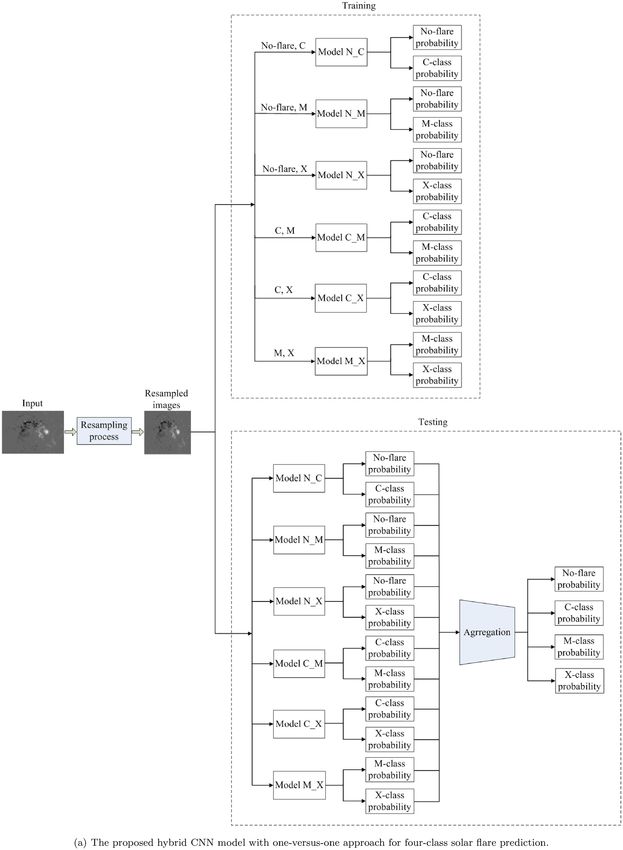
3520        Y. F. Zheng et al.
to deal with multiclass classification problems (Kang, Cho & Kang           still unbalanced at different classes. There are more No-flare/C-class
2015).                                                                      ARs than M/X-class ARs in our data sets.
   The computational process of CNN-based prediction models is to
split and combine various features from the raw solar observational
                                                                            3 METHOD
data, which are uninterpretable to humans, and thus CNN models are
usually considered as a black box (Yosinski et al. 2015). Such a black      Initially, we tried to train a single CNN model to predict four-class
box structure leads to the inability to explain the forecasting process     flares directly. However, the single CNN model showed large training
and the forecasting basis of the model. The feature visualization           loss during training, and then did not perform well during testing.
analysis is helpful to explain the feature parameters concerned by the      Therefore, we attempt to adopt the hybrid deep CNN model with one-
CNN model (Zeiler & Fergus 2014; Yosinski et al. 2015). However,            versus-one approach. The one-versus-one approach is to decompose
we have not found any researcher performed this aspect of research          an m-class classification problem into Cm2 = m(m − 1)/2 binary
from the existing literatures. We attempt for the first time to open the    classification tasks through pairwise combination. Each binary
black-box structure of the CNN flare prediction model by visualizing        classification task is managed by an independent binary classifier.

                                                                                                                                                           Downloaded from https://academic.oup.com/mnras/article/507/3/3519/6328501 by guest on 07 December 2021
the feature maps of different convolutional layers to study the image       All binary classifiers are trained by only the samples of the two
features that affect the prediction results.                                corresponding classes from the original training data set. In the
   The remainder of this paper is organized as follows. The data is         prediction or testing phase, each sample from the testing data set
described in Section 2, and the method is introduced in Section 3.          is submitted to all binary classifiers at the same time, and then the
Results are presented in Section 4, and conclusions and discussions         output result of these classifiers can be represented by the following
are provided in Section 5.                                                  score matrix P (Zhang et al. 2018a,b)
                                                                                  ⎡                    ⎤
                                                                                     − p12 · · · p1m
                                                                                  ⎢ p21 − · · · p2m ⎥
                                                                                  ⎢                    ⎥
2 DATA                                                                      P =⎢ .         .. . . .. ⎥,                                        (1)
                                                                                  ⎣ ..      .    .  . ⎦
The Helioseismic and Magnetic Imager (HMI; Schou et al. 2012) on                    pm1 pm2 · · · −
board the Solar Dynamics Observatory (SDO; Pesnell, Thompson &
Chamberlin 2012) began its routine observation on 2010 April 30.            where pij ∈ [0, 1] is the probability of the binary classifier discriminat-
SDO/HMI started to publicly release a new data product called Space-        ing class i from j in favour of the former class, while the probability
weather HMI Active Region Patches (SHARP; Bobra et al. 2014),               in favour of the latter can be calculated by pji = 1 − pij if the classifier
which can provide the LOS magnetograms of ARs. In this study, we            does not provide it. After the score matrix is obtained, the final output
adopt SHARP LOS magnetogram data from 2010 May 1 to 2018                    can be inferred by the aggregation strategies, such as majority voting
September 13, covering the main peak of solar cycle 24, as raw input        (Furnkranz 2002) and weighted voting (Galar et al. 2011). Previous
data for our prediction model. The magnetogram data of AR with              studies have proved that the weighted voting strategy is more robust
central longitudes located within ±45◦ of the central meridian is           and effective, so it is widely used as the most popular aggregation
included to avoid the influence of projection effects (Ahmed et al.         strategy (Hullermeier & Vanderlooy 2010; Galar et al. 2011). In our
2013; Bobra et al. 2014). The output result for our prediction model        work, we also adopt this aggregation strategy. In the weighted voting
is compared with the daily flare observations of the Geostationary          strategy, the total probability value of each class is calculated from
Operational Environment Satellite (GOES).                                   the score matrix P, and then the class with the largest total value is
   In order to assess the performance of our model properly, we need        chosen as the final output class. This process is implemented by the
to segregate the whole data set into the training and testing data set.     following formula:
The data sets we use are the same as used by Zheng et al. (2019),
because they adopt the method of shuffle and split cross-validation         class = arg max                 pij .                                    (2)
                                                                                         i=1,··· ,m
                                                                                                      1j =im
by ARs. This method ensures that the ARs and samples in the testing
data set do not appear in the training data set, which can effectively         We design the proposed hybrid CNN model with one-versus-
verify the validity and stability of the model. By using the same data      one approach in this study. The model is implemented in PYTHON
sets, we also can conduct fair performance comparisons between              programming language and the deep learning library KERAS with
different flare forecasting models. Initially, we collect 870 ARs and       TENSORFLOW (Abadi et al. 2016) as the backend. Fig. 1 shows
136 134 magnetogram samples, including 443 X-class, 6534 M-                 the proposed hybrid CNN model with one-versus-one approach
class, 72 412 C-class, and 56 745 No-flare magnetogram samples              and the architecture of our model consisting of six binary CNN
to build the data sets. It is clear that there is a significant imbalance   models. The proposed model adopts the one-versus-one approach to
in the number of samples at different classes. In order to alleviate        decompose the problem of four-class flare prediction into the sub-
this imbalance issue, we undersample No-flare/C-class samples by            problems of six binary class flare predictions. As shown in Fig. 1(a),
randomly selecting No-flare/C-class samples with about 2 samples            the proposed model is comprised of six different binary CNN
per 10 samples, and augment M/X-class samples by rotating and               models (Model N C, Model N M, Model N X, Model C M, Model
reflecting images. Table 1 shows the number of samples and ARs              C X, and Model M X), which are independent binary classifiers
for 10 separate data sets in our work. As can be seen from Table 1,         responsible for distinguishing between a different pair of classes.
through undersampling and data augmentation, the number of No-              The development of the proposed model involves two phases: a
flare/C-class samples is decreased, while the number of M/X-class           training phase and a prediction or testing phase. In the training
samples is increased. To some extent, the data imbalance is alleviated,     phase, each binary CNN model is trained independently by the subset
but the number of the samples is not equal at different classes. In         of training data sets including only the magnetogram samples of
addition, the undersampling and data augmentation techniques do             the two corresponding classes. Thus it generates the probabilities
not increase the number of ARs. Therefore, the number of ARs is             that the AR will produce a solar flare of the two corresponding

MNRAS 507, 3519–3539 (2021)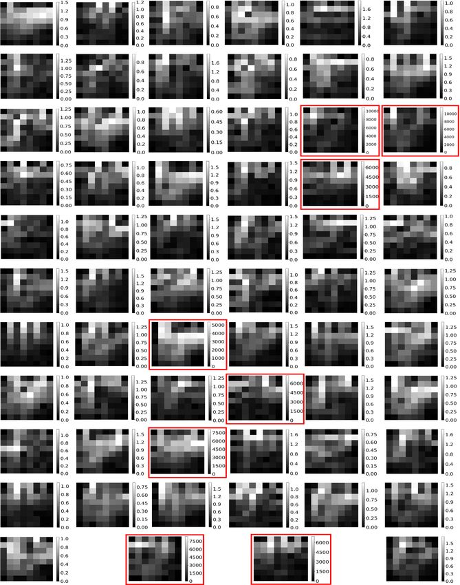
Hybrid deep CNN with OVO for flare prediction                         3521
              Table 1. The number of solar magnetogram samples and ARs for 10 separate data sets.

              Data set                   No-flare Class              C Class                 M Class                      X Class
                                      (Sample/AR numbers)      (Sample/AR numbers)     (Sample/AR numbers)          (Sample/AR numbers)

              No. 1: Training               8796/359                 11091/237                  8862/60                    2856/8
              Test                           1331/57                  1756/39                    1146/8                    1500/2
              Total                         10127/416                12847/276                 10008/68                   4356/10
              No. 2: Training               8824/351                 11242/235                  9408/60                   4080/8
              Test                           1733/72                  1589/36                    876/7                     60/1
              Total                         10557/423                12831/271                 10284/67                   4140/9
              No. 3: Training               8996/362                 11549/235                  8562/59                    4788/8
              Test                           1382/58                  1379/35                   1950/11                     312/2
              Total                         10378/420                12928/270                 10512/70                   5100/10

                                                                                                                                                     Downloaded from https://academic.oup.com/mnras/article/507/3/3519/6328501 by guest on 07 December 2021
              No. 4: Training               8807/347                 10864/239                  8814/60                   3684/8
              Test                           1565/66                  1635/37                    828/8                     1416/2
              Total                         10372/413                12499/276                  9642/68                   5100/10
              No. 5: Training               8951/352                 11611/234                  9270/59                    3756/8
              Test                           1664/68                  1686/38                    1218/9                     600/2
              Total                         10615/420                13237/272                 10488/68                   4356/10
              No. 6: Training               8836/359                 11189/238                  8580/62                   3648/8
              Test                           1500/62                  1641/39                    1332/5                    1668/3
              Total                         10336/421                12830/277                  9912/67                   5316/11
              No. 7: Training               8633/353                 11450/242                  8856/61                    3840/8
              Test                           1579/68                  1025/27                    1692/9                    1476/3
              Total                         10212/421                12475/269                 10548/70                   5316/11
              No. 8: Training               8908/357                 11689/243                  9468/58                    4632/8
              Test                           1459/64                   925/27                    750/7                      312/2
              Total                         10367/421                12614/270                 10218/65                   4944/10
              No. 9: Training               8964/359                 11398/241                  9174/62                    3504/8
              Test                           1413/61                  1473/34                    1038/5                    1440/2
              Total                         10377/420                12871/275                 10212/67                   4944/10
              No. 10: Training              8632/357                 11473/236                 9216/60                    3888/8
              Test                           1517/65                  1266/30                   1392/10                    252/1
              Total                         10149/422                12739/266                 10608/70                   4140/9

classes within 24 h. In the testing phase, each sample from the                 To maximize the prediction performance, all six different binary
testing data sets is input to all six binary CNN models evaluated            CNN models are iteratively trained on a small part of the training
simultaneously. Then each binary CNN model performs binary                   data set called a mini batch (Goodfellow, Bengio & Courville 2016)
class prediction and outputs the probabilities (i.e. pij and pji ) of        to minimize a loss function respectively. Since the number of ARs
the two corresponding classes, respectively. When all six binary             is imbalanced in our data sets, we employ the summation of a class-
CNN models complete the output probabilities, the score matrix P             weighted cross entropy as the loss function,
mentioned above can be acquired. Eventually, the proposed model
uses the weighted voting strategy to aggregate the output predictions
                                                                                   N
                                                                                     K−1

of all six binary CNN models, and calculates the final output                J =             Ck ynk loge (yˆnk ),                              (3)
                                                                                   n=1 k=0
class from the score matrix. Based on the final output class, the
proposed model makes four-class (i.e. No-flare, C, M, and X) flare           Ck = L(ARk )L(samplek )βk ,                                       (4)
prediction.
   All six different binary CNN models constituting the proposed             where K denotes the number of classes being equal to 2, N is the
hybrid CNN model utilize the same network architecture, which is             number of the training samples per mini batch, and ynk and yˆnk
illustrated in Fig. 1(b). In this study, after trying different combina-     represent the expected output and the forecasting output of the kth
tions of the following choices, such as the number of convolutional          class during a forward propagation, respectively. Ck is the weight
layers, filter size, and activation function, we adopt the binary CNN        of the kth class used for weighting the loss function, L(ARk ) is the
model architecture with the best performance. As the proposed hybrid         number of ARs of the kth class, and L(samplek ) is the number of
CNN model consists of six binary CNN models, it could achieve the            samples of the kth class. β k (k = 0, 1) is the optimized parameter
best performance for four-class prediction, in the case that these           used to adjust Ck , which is obtained through experiment and comes
six binary CNN models achieve the best performance for binary                in pairs of the corresponding two classes. In the training phase, the
class prediction. As shown in Fig. 1(b), each binary CNN model               parameters (such as weights and biases) of our models are iteratively
consists of 28 different layers and functions containing convolu-            updated to minimize the loss function using stochastic gradient
tional layers, pooling layers, dense layers, softmax layer, dropout          descent (SGD; LeCun et al. 1998a), where the gradients of the loss
layers, batch normalization (BN) layers, and ReLU activation                 function with respect to the weights and biases are calculated using
functions.                                                                   backpropagation procedure (Rumelhart, Hinton & Williams 1986).

                                                                                                                     MNRAS 507, 3519–3539 (2021)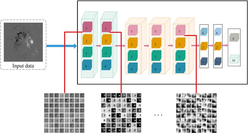
3522       Y. F. Zheng et al.

                                                                                                                                                  Downloaded from https://academic.oup.com/mnras/article/507/3/3519/6328501 by guest on 07 December 2021

    Figure 1. The proposed hybrid CNN model with one-versus-one approach and the architecture of our model consisting of six binary CNN models.

MNRAS 507, 3519–3539 (2021)
Hybrid deep CNN with OVO for flare prediction 3523
Downloaded from https://academic.oup.com/mnras/article/507/3/3519/6328501 by guest on 07 December 2021
Figure 1 – continued
4 R E S U LT S phenomenon could be alleviated by gradually decreasing the value
of learning rate. In our work, we select the learning rate parameter
4.1 Training results through the experiment to reduce the number of peaks as much as
possible. However, due to the difference of experimental data sets
We train and validate the six different binary CNN models that
used for training different models (Model N C, Model N M, Model
are combined to form the hybrid CNN model with one-versus-one
N X, Model C M, Model C X, and Model M X), there are still a few
approach by the training and validating data sets during each epoch
peaks on the loss curves in Figs 2(a), (e), and (g). In summary, it can
to track the learning performance. About 80 per cent of the samples
be found from Fig. 2 that both the training loss and validating loss
in the training data set is used to train each binary CNN model,
generally decrease with the increase in the number of epochs for all
and the remaining 20 per cent of the samples in the training data
binary CNN models. By checking the learning curves, we find that
set is used as the validation data set to validate the model. The
all binary CNN models are not subjected to the problems of poor
training and validation sets for each binary model contain only the
learning or serious overfitting.
samples in the full training and validation sets of the corresponding
two classes. We obtain 10 separate training and validation data sets
for training and validating the model in total. At the end of each
4.2 Testing results
epoch, we compute the loss function on the validating data set, and
the model that minimizes the validating loss is selected as the best The prediction results of the proposed hybrid CNN model can be
trained model, which is similar to previous studies (Huang et al. characterized by a confusion matrix. From this confusion matrix, we
2018; Park et al. 2018; Zheng et al. 2019). The learning curves for can calculate the following metrics (Zheng et al. 2019): precision,
the six different binary CNN models are illustrated in Fig. 2, giving recall, accuracy, false alarm ratio (FAR), Heidke skill score (HSS;
the training loss and validating loss with the respect to the number of Heidke 1926), and TSS. We use these metrics to evaluate the model
epochs, respectively. The 10 differently colored curves indicate the performance. The range of precision, recall, and accuracy is 0 to
variations in training and validating loss with epochs for the model 1, with the maximum value 1 being the perfect score. The range
trained and validated by 10 different data sets. In Figs 2(g) and (h), the of FAR is also 0 to 1, with the minimum value 0 being the perfect
peaks on the pink loss curves may be caused by the excessive changes score. HSS ranges from −∞ to 1, with 1 indicating perfect score and
in weights and biases of the model during the training process. This less than 0 indicating no skill. TSS ranges from −1 (for no correct
MNRAS 507, 3519–3539 (2021)3524 Y. F. Zheng et al.
Downloaded from https://academic.oup.com/mnras/article/507/3/3519/6328501 by guest on 07 December 2021
Figure 2. Learning curves showing the training loss and validating loss with the respect to the number of epochs for the six different binary CNN models. The
10 differently colored curves indicate the variations in training and validating loss with epochs for the model trained and validated by 10 different data sets.
MNRAS 507, 3519–3539 (2021)Hybrid deep CNN with OVO for flare prediction 3525
Downloaded from https://academic.oup.com/mnras/article/507/3/3519/6328501 by guest on 07 December 2021
Figure 2 – continued
predictions) to +1 (for all correct predictions) and a value of zero 2015). Therefore, we also follow the suggestion of Bloomfield et al.
indicates that the predictions have been generated mainly by chance. (2012) to use the TSS as primary metric.
Among the above six metrics, only the TSS score is insensitive to We evaluate or test the proposed hybrid CNN model with one-
the class imbalance ratio (Bloomfield et al. 2012; Bobra & Couvidat versus-one approach on each of 10 testing data sets to obtain
MNRAS 507, 3519–3539 (2021)3526 Y. F. Zheng et al.
Downloaded from https://academic.oup.com/mnras/article/507/3/3519/6328501 by guest on 07 December 2021
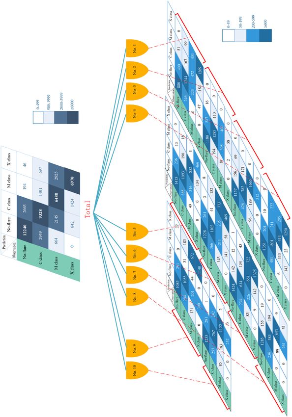
Figure 3. The confusion matrices for the proposed model evaluated on each of 10 data sets.
MNRAS 507, 3519–3539 (2021)Hybrid deep CNN with OVO for flare prediction 3527
Table 2. The four-class flare prediction results of our proposed hybrid CNN model (within 24 h) and comparison to previous studies.
Metric Model No-flare (weaker than C1.0) Class C Class M Class X Class
Recall This work 0.807 ± 0.076 0.644 ± 0.083 0.518 ± 0.272 0.523 ± 0.398
Zheng et al. (2019) 0.869 ± 0.034 0.671 ± 0.059 0.617 ± 0.148 0.594 ± 0.394
Liu et al. (2017) 0.812 ± 0.039 0.526 ± 0.050 0.671 ± 0.037 0.297 ± 0.039
Bloomfield et al. (2012) – 0.737 0.693 0.859
Colak & Qahwaji (2009) – 0.772 0.865 0.917
Precision This work 0.773 ± 0.045 0.638 ± 0.041 0.659 ± 0.060 0.502 ± 0.346
Zheng et al. (2019) 0.793 ± 0.054 0.670 ± 0.079 0.699 ± 0.087 0.562 ± 0.383
Liu et al. (2017) 0.703 ± 0.037 0.563 ± 0.054 0.656 ± 0.036 0.745 ± 0.152
Bloomfield et al. (2012) – 0.330 0.136 0.029
Colak & Qahwaji (2009) – – – –
Downloaded from https://academic.oup.com/mnras/article/507/3/3519/6328501 by guest on 07 December 2021
Accuracy This work 0.869 ± 0.027 0.791 ± 0.039 0.830 ± 0.031 0.893 ± 0.065
Zheng et al. (2019) 0.891 ± 0.018 0.812 ± 0.029 0.849 ± 0.034 0.933 ± 0.041
Liu et al. (2017) 0.844 ± 0.017 0.712 ± 0.026 0.778 ± 0.019 0.957 ± 0.005
Bloomfield et al. (2012) – 0.711 0.829 0.881
Colak & Qahwaji (2009) – 0.811 0.944 0.981
FAR This work 0.226 ± 0.045 0.361 ± 0.041 0.340 ± 0.060 0.297 ± 0.281
Zheng et al. (2019) 0.207 ± 0.054 0.330 ± 0.079 0.301 ± 0.087 0.138 ± 0.140
Liu et al. (2017) 0.297 ± 0.023 0.437 ± 0.016 0.344 ± 0.020 0.255 ± 0.126
Bloomfield et al. (2012) – 0.670 0.864 0.971
Colak & Qahwaji (2009) – 0.319 0.688 0.967
HSS This work 0.692 ± 0.058 0.488 ± 0.047 0.444 ± 0.194 0.419 ± 0.309
Zheng et al. (2019) 0.747 ± 0.037 0.535 ± 0.061 0.551 ± 0.120 0.539 ± 0.366
Liu et al. (2017) 0.640 ± 0.032 0.334 ± 0.028 0.497 ± 0.031 0.406 ± 0.014
Bloomfield et al. (2012) – 0.296 0.177 0.049
Colak & Qahwaji (2009) – 0.493 0.470 0.169
TSS This work 0.703 ± 0.070 0.489 ± 0.049 0.432 ± 0.222 0.436 ± 0.330
Zheng et al. (2019) 0.768 ± 0.028 0.538 ± 0.059 0.534 ± 0.137 0.552 ± 0.370
Liu et al. (2017) 0.669 ± 0.039 0.328 ± 0.050 0.500 ± 0.037 0.291 ± 0.039
Bloomfield et al. (2012) – 0.443 0.526 0.740
Colak & Qahwaji (2009) – – – –
Note. For Liu et al. (2017) and Zheng et al. (2019), we use the results provided by Zheng et al. (2019) in their table 3. Colak & Qahwaji (2009)
did not provide the scores of TSS and Precision. The scores we show are average in this table, but the results of Bloomfield et al. (2012) are their
optimum result and not an average.
the prediction result. Fig. 3 shows the confusion matrices for the for four-class flare prediction. Table 3 shows the prediction results of
proposed model evaluated on each of 10 data sets. The values in our proposed hybrid CNN model within 24 h for ≥C class and ≥M
each confusion matrix represent the numbers of samples predicted class, which are compared with previous studies. For ≥C class and
correctly (primary diagonal) and incorrectly (off the primary di- ≥M class prediction, the TSS score of the model is 0.703 ± 0.070
agonal). The total confusion matrix (i.e. the top matrix in Fig. 3) and 0.739 ± 0.109, respectively, which is obviously superior to that
is derived from the summation of these 10 confusion matrices. The of Huang et al. (2018) and Park et al. (2018), but a little smaller than
four-class flare prediction results of our proposed hybrid CNN model that of Zheng et al. (2019). Overall, experimental results demonstrate
within 24 h are presented and compared with previous studies in that the predictive performance of our proposed hybrid CNN model
recent years in Table 2. The model in our work and the model of with one-versus-one approach is close to that of Zheng et al. (2019)
Zheng et al. (2019) give the means and standard deviations of the while being superior to all the others for both multiclass prediction
performance metrics based on different CNN methods using the and binary class prediction.
same data sets. The average TSS scores of our model are 0.703,
0.489, 0.432, and 0.436 for No-flare, C, M, and X class, respectively,
4.3 Feature visualization
which are slightly smaller than those of Zheng et al. (2019). Our
average TSS scores are better than those of Liu et al. (2017) in each In our study, the effectiveness of our prediction model is verified by
class except for M class. We show average scores in Table 2, but the above experiments. However, CNN models are always known
Bloomfield et al. (2012) only show their optimum result which is not as black boxes. Understanding what current solar flare forecasting
an average. Our optimum TSS scores are 0.726, 0.489, 0.614, and model based on CNNs have learned is a key way to further improve
0.772 for No-flare, C, M, and X class, respectively, which are better it. Thus, in order to interpret why the model can work well, it is
than those of Bloomfield et al. (2012). It can be seen from Table 2 necessary to visualize what the model learns by feature maps and
that in addition to the TSS, we obtain quite good scores in other five then give a qualitative empirical analysis (Zeiler & Fergus 2014;
metrics at the same time. Based on the same data sets, our model Yosinski et al. 2015). We modify the loss function by abandoning
can also make binary class prediction for solar flares. The result for the weight Ck in Equation (3), and keep the training and validation
binary class prediction can be derived from the confusion matrices splits, initial weights, and other factors unchanged to obtain a
MNRAS 507, 3519–3539 (2021)3528 Y. F. Zheng et al.
Table 3. The flare prediction results of our proposed hybrid CNN model (within 24 h) for
≥C class and ≥M class and comparison to previous studies.
Metric Model ≥C Class ≥M Class
Recall This work 0.895 ± 0.024 0.818 ± 0.120
Zheng et al. (2019) 0.898 ± 0.030 0.817 ± 0.084
Huang et al. (2018) 0.726 0.850
Park et al. (2018) 0.85 –
Precision This work 0.913 ± 0.041 0.873 ± 0.044
Zheng et al. (2019) 0.939 ± 0.019 0.889 ± 0.056
Huang et al. (2018) 0.352 0.101
Park et al. (2018) – –
Accuracy This work 0.869 ± 0.027 0.887 ± 0.026
Downloaded from https://academic.oup.com/mnras/article/507/3/3519/6328501 by guest on 07 December 2021
Zheng et al. (2019) 0.891 ± 0.017 0.891 ± 0.024
Huang et al. (2018) 0.756 0.813
Park et al. (2018) 0.82 –
FAR This work 0.086 ± 0.041 0.126 ± 0.044
Zheng et al. (2019) 0.060 ± 0.019 0.111 ± 0.056
Huang et al. (2018) 0.648 0.899
Park et al. (2018) 0.17 –
HSS This work 0.692 ± 0.058 0.746 ± 0.089
Zheng et al. (2019) 0.746 ± 0.037 0.759 ± 0.071
Huang et al. (2018) 0.339 0.143
Park et al. (2018) 0.63 –
TSS This work 0.703 ± 0.070 0.739 ± 0.109
Zheng et al. (2019) 0.767 ± 0.028 0.749 ± 0.079
Huang et al. (2018) 0.487 0.662
Park et al. (2018) 0.63 –
Note. For Zheng et al. (2019), we compute all six metric scores from the confusion matrices in
table 4 they provided. For Huang et al. (2018), we calculate the scores of Precision, Accuracy,
and FAR from the contingency table in table 4 they provided.
new model. We train and evaluate the model again, and obtain layer of the model. The natural logarithmic values of the gradient
the following results. The TSS score of low-performance model median for the high-level feature maps output by 64 filters are
is 0.527 ± 0.066, 0.142 ± 0.075, 0.279 ± 0.075, −0.027 ± 0.073 given in Fig. A1(a). From Fig. A1, we obtain the following results:
for No-flare, C, M, and X class, respectively. As shown in Fig. 4, (1) the median values of gradients of the area concerned by the
we perform feature visualization for both high-performance model high-performance model are significantly higher than those of the
and low-performance model respectively, and obtain the feature low-performance model, which applies not only to one AR sample,
images output by each convolution layer of the model respectively. but also to other AR samples. (2) The median values of the gradients
As shown in Figs 4(b)–(c) and (f)–(g), the low-level features, e.g. concerned by both high-performance model and low-performance
the edges or shape, of the input image are detected in the lower model increase approximately with the increase of flare level. The
convolutional layers, which are still recognizable. Subsequent layers relationship between the magnitude of the gradient values and the
use these low-level features to detect higher level features. As shown flare level can be clearly seen in Fig. A1(b). (3) In addition, we
in Figs 4(d) and (h), high-level image features are detected in the calculate the median values of the intensity, total intensity, and the
last convolutional layer, which become more abstract and difficult to range of intensity values for the feature map images from the last
explain. convolutional layer as shown in Figs A1(c)–(h), and they behave sim-
By investigating the 64 feature map images output by each ilarly to the gradients in the high-performance and low-performance
convolutional layer of the high-performance and low-performance models.
models, we find the following two characteristics: firstly, there is no In addition, we find from Figs A1(a), (c), (e) and (g) that there are
significant difference in terms of feature distribution (e.g. the edges a few peaks for the 64 filters corresponding to each AR sample in the
or shape) in the lower convolutional layers of the high-performance low performance prediction. To investigate the source of these peaks
and low-performance models, especially in the first convolutional and their rationality, we examine all feature visualization images, as
layer. Secondly, by comparing the dynamic range of the data, we shown in Fig. A2. Figs A2(a)–(c) present the feature map images
find that the range in the high performance prediction is significantly output by the first, second, and fifth convolutional layers of the
higher than that in the low performance prediction, especially in low-performance model respectively, and Fig. A2(d) presents the
the last convolutional layer. Since the final output result of the gradient images for the feature maps of Fig. A2(c). As shown in
prediction model mainly depends on the image features output by Fig. A2(a), two of the output images from the 64 filters in the first
the last convolutional layer, we randomly select 10 different AR convolutional layer exhibit image features with large dynamic range
samples for each class as the input of the model, and calculate the of the data which are distinctly different from those of the other
gradient values for the feature maps output by the last convolutional images, and these features are similar to those visualized by the
MNRAS 507, 3519–3539 (2021)Hybrid deep CNN with OVO for flare prediction 3529
Downloaded from https://academic.oup.com/mnras/article/507/3/3519/6328501 by guest on 07 December 2021
Figure 4. Feature visualization. (a) shows the normalized AR image as the input of the the model, which is the LOS magnetogram sample of X-class AR 11890
observed at 19:36 UT on 2013 November 7. (b)–(d) present one of the feature map images output by the first, second, and fifth convolutional layers of the
high-performance model respectively, and (f)–(h) correspondingly present one of the feature map images output by the low-performance model. We find that
the output image from the fifth convolutional layer shows a strong contrast. Therefore, we calculate the gradient for the output image from the last convolutional
layer, and (e) and (i) show the gradient images for the feature maps of (d) and (h) respectively. The values on the colorbars for (a)–(i) can be clearly seen by
zooming in.
high-performance model.1 As shown in Figs A2(b) and (c), five weights and spatial or temporal undersampling to ensure a degree of
images similar to the visualized results of the high-performance displacement, scale and deformation invariance. From the second
model appear in the second convolutional layer and eight images in convolutional layer, each unit in a layer receives inputs from a
the fifth convolutional layer. The number of visualized images with set of units located in a small neighborhood in the previous layer
distinctive features from the last convolutional layer is consistent (LeCun et al. 1998b). In other words, each unit in each feature map
with the number of peaks in Fig. A1. A similar phenomenon is is connected to several small neighborhoods at identical locations in
also observed for the other 9 AR samples. This is because CNNs a subset of feature maps in previous layer. In the low performance
combine the three structural concepts of local receptive fields, shared prediction, the first convolutional layer acquires some of the features
that affect the correct forecasting results. These feature images and
the neighbourhood images are combined into multiple feature sets,
1 https://github.com/FlarePrediction/Repository/tree/papers/paper11/MNRA which are used as input of the next convolutional layer, corresponding
S V2/Figure%20C to a certain number of outputs. As the number of convolutional layers
MNRAS 507, 3519–3539 (2021)3530 Y. F. Zheng et al.
increases, the number of features learned that are relevant to the as class M, while some of M-class samples are mostly incorrectly
correct prediction result also increases, so that the low-performance predicted as class X. This indicates that the correct predictions of
model can also obtain some correct predictions. ≥M-class major flares are not missed, which does not degrade
the performance of the model for ≥M-class prediction. Based on
our experimental results, we conclude that the proposed hybrid
5 CONCLUSIONS AND DISCUSSIONS
CNN model with one-versus-one approach is an effective method
In this study, we propose a new hybrid deep CNN model with for the solar flare prediction task. In near future work, with the
one-versus-one approach to forecast solar flare occurrence with the continued observation of SDO/HMI, we would gather more X-class
outputs of four classes (i.e. No-flare, C, M, and X) within 24 h. ARs and samples in the data sets to improve the model robustness for
The proposed model decomposes the problem of four-class flare predicting M/X-class flares. However, waiting for more X-class flares
prediction into the sub-problems of six binary class predictions by to use for training is a very slow process. It is worthwhile exploring
the one-versus-one approach, which are managed by six different other data augmentation techniques, such as generative adversarial
binary CNN models respectively. We train these binary CNN models networks (GANs; Kim et al. 2019) to gain more X-class AR samples.
Downloaded from https://academic.oup.com/mnras/article/507/3/3519/6328501 by guest on 07 December 2021
independently in the training phase, and then aggregate the output We will also try other methods, such as including domain knowledge
predictions of binary models by the weighted voting strategy to into the fully-connected network, to further improve the predictive
obtain a final prediction result in the testing phase. The main results performance of the model. In addition, our current hybrid CNN
of this paper are summarized as follows. (1) To our knowledge, this model can process time-series data, but it does not use the linear
is the first time that the CNN model in conjunction with one-versus- relationship for analysis, which is a very important problem in the
one approach has been used in solar physics to make multiclass process of flare prediction. The long short-term memory (LSTM)
forecasting for solar flares. (2) In the multiclass flare prediction, our networks can compute the dependencies between time-series data
model achieves relatively high average scores of TSS = 0.703, 0.489, and are often used to solve time-series prediction problem. Our next
0.432, and 0.436 for No-flare, C, M, and X class, respectively. In the step work is to develop the model with CNNs and LSTM networks
binary class prediction, the TSS score of our model is 0.703 ± 0.070 to deal with time-series images and further improve the performance
for ≥C-class prediction and 0.739 ± 0.109 for ≥M-class prediction, of flare prediction.
respectively. (3) According to the literature, this is the first attempt
to open the black-box CNN model to visualize the feature maps
AC K N OW L E D G E M E N T S
for interpreting the flare prediction model. In addition, the results
of feature visualization demonstrate that the prediction performance We wish to thank the anonymous referee for valuable suggestions
of our model is related to the gradient, the intensity, total intensity, and comments that improved this work significantly. We thank the
and the range of the intensity in feature maps of deeper layer, which Solar Dynamics Observatory/Helioseismic and Magnetic Imager
increase approximately with the increase of flare level. It is worth (SDO/HMI) team members who have made contributions to the
noting that the median gradient concerned by both high-performance SDO mission for their hard work. This work is supported by
model and low-performance model increases approximately as the the National Natural Science Foundation of China (Grants No.
flare level increases. Exploring this further would be worthwhile in 11703009, No.11803010), the Natural Science Foundation of Jiangsu
follow-up work as it may lead to insights into improving the network. Province, China (Grant No. BK20170566, No. BK20201199), and
Many previous studies point out solar flares are closely related to the the Qing Lan Project.
physical features extracted from near the polarity inverse line (PIL) in
the photospheric magnetic field, which are used for flare forecasting
DATA AVA I L A B I L I T Y
(e.g. Cui et al. 2006; Georgoulis & Rust 2007; Schrijver 2009;
Bobra & Couvidat 2015; Liu et al. 2017). Cui et al. (2006) believe The data underlying this article are available in the article and
that solar flares are correlated with the maximum horizontal gradient in its online supplementary material, which are also available
and the length of the neutral line. Schrijver (2009) reviews that large in https://github.com/FlarePrediction/Repository/tree/papers/paper1
flares tend to occur in the AR with strong magnetic field gradient 1/MNRAS V2. The data sets used in the paper are large, with
and long PIL. Bobra & Couvidat (2015) utilize dozens of physical compression up to about 5.23GB, so we provide the website
features including magnetic field gradients to predict solar flares. information for downloading. You may need to register a user for
Georgoulis & Rust (2007) define the effective connected magnetic the BaiduNetDisk, and then download the data sets according to the
field intensity to measure the flaring potential in ARs. Liu et al. information of the readme file in the supplementary material.
(2017) discover that flux near the PIL is one of the most important
features for predicting solar flares. Therefore, in combination with
REFERENCES
our finding, we speculate that our flare prediction model concentrates
on the regions with strong magnetic field gradient, strong magnetic Abadi M. et al., 2016, preprint (arXiv:1603.04467)
field intensity, high total magnetic field intensity, and large variation Ahmed O. W., Qahwaji R., Colak T., Higgins P.A., Gallagher P.T., Bloomfield
range of magnetic field intensity, which is in agreement with previous D.S., 2013, Sol. Phys., 283, 157
studies. Barnes G. et al., 2016, ApJ, 829, 89
It can be found from Table 2 that the standard deviations of the Bloomfield D. S., Higgins P. A., James McAteer R. T., Gallagher P. T., 2012,
ApJ, 747, L41
metrics for M class and X class are larger, implying that our model
Bobra M. G., Couvidat S., 2015, ApJ, 798, 135
is not very stable in predicting M/X-class flares in the multiclass
Bobra M. G., Sun X., Hoeksema J. T., Turmon M., Liu Y., Hayashi K., Barnes
flare forecasting. This is because our model has some difficulty G., Leka K. D., 2014, Sol. Phys., 289, 3549
in distinguishing between M-class and X-class samples, mostly Cinto T., Gradvohl A. L. S., Coelho G. P., Silva A. E. A. da, 2020, MNRAS,
resulting from the shortage of X-class ARs and samples in the solar 495, 3332
cycle 24. Fortunately, from the confusion matrices in Fig. 3, it can be Colak T., Qahwaji R., 2009, Space Weather, 7, S06001
found that some of X-class samples are mostly incorrectly predicted Cui Y. M., Li R., Zhang L. Y., He Y., Wang H., 2006, Sol. Phys., 237, 45
MNRAS 507, 3519–3539 (2021)Hybrid deep CNN with OVO for flare prediction 3531
Florios K., Kontogiannis I., Park S. H., Guerra J.A., Benvenuto F., Bloomfield Qahwaji R., Colak T., 2007, Sol. Phys., 241, 195
D.S., Georgoulis M.K., 2018, Sol. Phys., 293, 28 Rumelhart D. E., Hinton G. E., Williams R. J., 1986, Nature, 323, 533
Furnkranz J., 2002, J. Mach. Learn. Res., 2, 721 Sadykov V. M., Kosovichev A. G., 2017, ApJ, 849, 148
Galar M., Fernandez A., Barrenechea E., Bustince H., Herrera F., 2011, Schou J. et al., 2012, Sol. Phys., 275, 229
Pattern Recognit., 44, 1761 Schrijver C. J., 2009, Adv. Space Res., 43, 739
Georgoulis M. K., Rust D. M., 2007, ApJ, 661, L109 Song H., Tan C., Jing J., Wang H., Yurchyshyn V., Abramenko V., 2009, Sol.
Goodfellow I., Bengio Y., Courville A., 2016, Deep Learning. MIT Press, Phys., 254, 101
Cambridge. Available at: http://www.deeplearningbook.org/ Yosinski J., Clune J., Nguyen A., Fuchs T., Lipson H., 2015, in Deep Learning
Guerra J. A., Pulkkinen A., Uritsky V. M., 2015, Space Weather, 13, Workshop, Proc. 31th Int. Conf. on Machine Learning. ICML-15, Lille
626 Yuan Y., Shih F. Y., Jing J., Wang H. M., 2010, Res. Astron. Astrophys., 10,
Hanssen A. W., Kuipers W. J. A., 1965, Meded. Verh., 81, 2 785
Heidke P., 1926, Geogr. Ann., 8, 301 Zeiler M. D., Fergus R., 2014, in European Conference on Computer Vision.
Huang X., Yu D. R., Hu Q. H., Wang H. N., Cui Y. M., 2010, Sol. Phys., 263, Springer, Berlin, p. 818
175 Zhang Z. L., Luo X. G., Garcia S., Tang J. F., Herrera F., 2017, Knowl.-Based
Downloaded from https://academic.oup.com/mnras/article/507/3/3519/6328501 by guest on 07 December 2021
Huang X., Zhang L., Wang H., Li L., 2013, A&A, 549, A127 Syst., 125, 53
Huang X., Wang H., Xu L., Liu J., Li R., Dai X., 2018, ApJ, 856, 7 Zhang Z. L., Luo X. G., Gonzalez S., Garcia S., Herrera F., 2018a,
Hullermeier E., Vanderlooy S., 2010, Pattern Recognit., 43, 128 Neurocomputing, 285, 176
Kang S. K., Cho S., Kang P., 2015, Neurocomputing, 149, 677 Zhang Z. L., Luo X. G., Yu Y., Yuan B. W., Tang J. F., 2018b, Eng. Appl.
Kim T. et al., 2019, Nature Astron., 3, 397 Artif. Intel., 74, 43
LeCun Y., Bottou L., Orr G. B., Müller K.-R., 1998a, in Montavon G., Orr Zheng Y. F., Li X. B., Wang X. S., 2019, ApJ, 885, 73
G., Müller K.-R., eds, Neural Networks: Tricks of the Trade. Springer,
Berlin, p. 9
LeCun Y., Bottou L., Bengio Y., Haffner P., 1998b, Proc. IEEE, 86, 2278 S U P P O RT I N G I N F O R M AT I O N
LeCun Y., Bengio Y., Hinton G., 2015, Nature, 521, 436
Supplementary data are available at MNRAS online.
Leka K. D., Barnes G., Wagner E., 2018, J. Space Weather Space Clim., 8,
A25 Supplementary material.zip
Li R., Zhu J., 2013, Res. Astron. Astrophys., 13, 1118
Li R., Cui Y., He H., Wang H., 2008, Adv. Space Res., 42, 1469 Please note: Oxford University Press is not responsible for the content
Liu C., Deng N., Wang J. T. L., Wang H. M., 2017, ApJ, 843, 104 or functionality of any supporting materials supplied by the authors.
Mason J. P., Hoeksema J. T., 2010, ApJ, 723, 634 Any queries (other than missing material) should be directed to the
Muranushi T., Shibayama T., Muranushi Y. H., Yuko H., Isobe H., Nemoto corresponding author for the article.
S., Komazaki K., Shibata K., 2015, Space Weather, 13, 778
Nishizuka N., Sugiura K., Kubo Y., Den M., Watari S., Ishii M., 2017, ApJ,
835, 156 A P P E N D I X A : F E AT U R E V I S UA L I Z AT I O N
Nishizuka N., Sugiura K., Kubo Y., Den M., Ishii M., 2018, ApJ, 858, 113
Park E., Moon Y. J., Shin S., Yi K., Lim D., Lee H., Shin G., 2018, ApJ, 869, In Fig. A1, we present the results of feature visualization. In Fig. A2,
91 we show the feature maps output by different convolutional layers of
Pesnell W. D., Thompson B. J., Chamberlin P. C., 2012, Sol. Phys., 275, 3 the low-performance model.
MNRAS 507, 3519–3539 (2021)3532 Y. F. Zheng et al.
Downloaded from https://academic.oup.com/mnras/article/507/3/3519/6328501 by guest on 07 December 2021
Figure A1. The results of feature visualization. (a), (c), (e), and (g) show the logarithmic values of median gradient, median intensity, total intensity, and the
range of the intensity for the feature maps from the last convolutional layer in high-performance model and in low-performance model, respectively, using 10
different AR samples with four classes. (b), (d), (f), and (h) show the values of median gradient, median intensity, total intensity, and the range of the intensity
for the feature maps from the last convolutional layer in high-performance model, respectively.
MNRAS 507, 3519–3539 (2021)Downloaded from https://academic.oup.com/mnras/article/507/3/3519/6328501 by guest on 07 December 2021
3533
MNRAS 507, 3519–3539 (2021)
Hybrid deep CNN with OVO for flare prediction
Figure A1 – continuedDownloaded from https://academic.oup.com/mnras/article/507/3/3519/6328501 by guest on 07 December 2021
Figure A1 – continued
Y. F. Zheng et al.
MNRAS 507, 3519–3539 (2021)
3534Downloaded from https://academic.oup.com/mnras/article/507/3/3519/6328501 by guest on 07 December 2021
3535
MNRAS 507, 3519–3539 (2021)
Hybrid deep CNN with OVO for flare prediction
Figure A1 – continued3536 Y. F. Zheng et al.
Downloaded from https://academic.oup.com/mnras/article/507/3/3519/6328501 by guest on 07 December 2021
Figure A2. The feature maps output by different convolutional layers of the low-performance model. The raw input corresponding to these feature maps is the
LOS magnetogram sample of X-class AR 11890 observed at 19:36 UT on 2013 November 7. (a)–(c) show the feature map images output by the first, second,
and fifth convolutional layers of the low-performance model respectively, and (d) shows the gradient images for the feature maps of (c). The feature maps with
red boxes show different image features from the others. The values on the colorbars for (a)–(d) can be clearly seen by zooming in.
MNRAS 507, 3519–3539 (2021)Downloaded from https://academic.oup.com/mnras/article/507/3/3519/6328501 by guest on 07 December 2021
3537
MNRAS 507, 3519–3539 (2021)
Hybrid deep CNN with OVO for flare prediction
Figure A2 – continuedDownloaded from https://academic.oup.com/mnras/article/507/3/3519/6328501 by guest on 07 December 2021
Figure A2 – continued
Y. F. Zheng et al.
MNRAS 507, 3519–3539 (2021)
3538Hybrid deep CNN with OVO for flare prediction 3539
Downloaded from https://academic.oup.com/mnras/article/507/3/3519/6328501 by guest on 07 December 2021
Figure A2 – continued
This paper has been typeset from a TE
X/LAT
EX file prepared by the author.
MNRAS 507, 3519–3539 (2021)You can also read