IGAPS: the merged IPHAS and UVEX optical surveys of the Northern Galactic Plane
←
→
Page content transcription
If your browser does not render page correctly, please read the page content below
Astronomy & Astrophysics manuscript no. main                                                                                         c ESO 2020
                                               February 13, 2020

                                                       IGAPS: the merged IPHAS and UVEX optical surveys of the
                                                                       Northern Galactic Plane
                                                 M. Monguió1, 2 , R. Greimel3 , J. E. Drew1, 4 , G. Barentsen1, 5 , P. J. Groot6, 7, 8, 9 , M. J. Irwin10 , J. Casares11, 12 , B. T.
                                                Gänsicke13 , P. J. Carter13, 14 , J. M. Corral-Santana11, 15 , N. P. Gentile-Fusillo13, 15 , S. Greiss13 , L. M. van Haaften6, 16 ,
                                                M. Hollands13 , D. Jones11, 12 , T. Kupfer6, 17 , C. J. Manser13 , D. N. A. Murphy10 , A. F. McLeod6, 16, 18 , T. Oosting6 , Q.
                                                  A. Parker19 , S. Pyrzas13, 20 , P. Rodríguez-Gil11, 12 , J. van Roestel6, 21 , S. Scaringi16 , P. Schellart6 , O. Toloza13 , O.
                                                Vaduvescu11, 22 , L. van Spaandonk13, 23 , K. Verbeek6 , N. J. Wright24 , J. Eislöffel25 , J. Fabregat26 , A. Harris1 , R. A. H.
                                                  Morris27 , S. Phillipps27 , R. Raddi13, 28 , L. Sabin29 , Y. Unruh30 , J. S Vink31 , R. Wesson4 , A. Cardwell22, 32 , R. K.
                                                Cochrane22 , S. Doostmohammadi22, 33 , T. Mocnik22 , H. Stoev22 , L. Suárez-Andrés22 , V. Tudor22 , T. G. Wilson22 , and
arXiv:2002.05157v1 [astro-ph.IM] 12 Feb 2020

                                                                                                         T. J. Zegmott22
                                                                                                 (Affiliations can be found after the references)

                                                                                           Received December 17, 2019; accepted February 12, 2020

                                                                                                                  ABSTRACT

                                               The INT Galactic Plane Survey (IGAPS) is the merger of the optical photometric surveys, IPHAS and UVEX, based on data from the Isaac Newton
                                               Telescope (INT) obtained between 2003 and 2018. Here, we present the IGAPS point source catalogue. It contains 295.4 million rows providing
                                               photometry in the filters, i, r, narrow-band Hα, g and URGO . The IGAPS footprint fills the Galactic coordinate range, |b| < 5◦ and 30◦ < ` < 215◦ .
                                               A uniform calibration, referred to the Pan-STARRS system, is applied to g, r and i, while the Hα calibration is linked to r and then is reconciled
                                               via field overlaps. The astrometry in all 5 bands has been recalculated on the Gaia DR2 frame. Down to i ∼ 20 mag. (Vega system), most stars
                                               are also detected in g, r and Hα. As exposures in the r band were obtained within the IPHAS and UVEX surveys a few years apart, typically, the
                                               catalogue includes two distinct r measures, rI and rU . The r 10σ limiting magnitude is ∼21, with median seeing 1.1 arcsec. Between ∼13th and
                                               ∼19th magnitudes in all bands, the photometry is internally reproducible to within 0.02 magnitudes. Stars brighter than r = 19.5 have been tested
                                               for narrow-band Hα excess signalling line emission, and for variation exceeding |rI − rU | = 0.2 mag. We find and flag 8292 candidate emission
                                               line stars and over 53000 variables (both at > 5σ confidence). The 174-column catalogue will be available via CDS Strasbourg.
                                               Key words. stars: general – stars: evolution – Galaxy: disc – surveys – catalogues

                                               1. Introduction                                                            of the northern Galactic Plane, Groot et al. 2009) has included
                                                                                                                          imaging using the Sloan-u-like URGO filter. In concept, these two
                                               The stellar and nebular content of the Galactic Plane continues            surveys are the older siblings to VPHAS+, the survey covering
                                               to be a vitally important object of study as it offers the best avail-     the southern Galactic Plane and Bulge (Drew et al. 2014).
                                               able angular resolution to understand how galactic disc environ-               A crucial and defining feature of the IPHAS and UVEX sur-
                                               ments are built, interact and evolve over time. The optical part           veys is that their observing plans centered on contemporaneous
                                               of the electromagnetic spectrum remains an important window,               observations in the full set of filters so as to achieve faithful
                                               particularly for characterising the properties of the disc’s stellar       colour information, immune to stellar variability on timescales
                                               content, as this is the range in which the Planck function maxi-           longer than ∼10 minutes. This characteristic is shared with the
                                               mum falls for most stars. For studies of the interstellar medium,          continuing Gaia mission (Gaia Collaboration et al. 2018). Both
                                               it is relevant that the optical is also the domain in which Hα, the        IPHAS and UVEX were executed using the Wide Field Cam-
                                               strongest observable hydrogen emission line, is located. This line         era (WFC) on the Isaac Newton Telescope (INT) in La Palma.
                                               is the outstanding tracer of ionized interstellar and circumstellar        Together they form the largest scientific investigation so far un-
                                               gas.                                                                       dertaken at the INT, requiring more than 400 nights.
                                                   In this era of digital surveys, there is a growing menu of                 IPHAS and UVEX are respectively red-optical and blue-
                                               ground-based wide-field optical broad band surveys covering                optical surveys. So that they could be linked together, photo-
                                               much of the sky, north and south (SDSS, Pan-STARRS, APASS,                 metrically, both surveys included the Sloan r band in their filter
                                               DECaPS, Skymapper, see: Alam et al. 2015; Chambers et al.                  sets. This was also seen as an opportunity to look for evidence of
                                               2016; Henden et al. 2015; Schlafly et al. 2018; Wolf et al. 2018).         both variability and measurable proper motion relative to a typi-
                                               Here we add to the menu by focusing on the dense star fields               cal epoch difference of a few years. We note that recent work by
                                               of the northern Milky Way, and by bring together for the first             Scaringi et al. (2018) has already identified higher proper motion
                                               time, two Galactic Plane surveys that have each deployed a fil-            objects by comparing IPHAS r and Gaia DR2 positions. Here we
                                               ter particularly well suited to searching for early and late phases        will briefly consider the incidence of variability as revealed by
                                               of stellar evolution. IPHAS (The INT Photometric Hα survey of              the two epochs of IPHAS and UVEX r band data.
                                               the northern Galactic Plane, Drew et al. 2005) has incorporated                This paper presents a calibration of the point source pho-
                                               imaging narrow-band Hα, while UVEX (The UV-Excess survey                   tometry in r/i/Hα and r/g/URGO collected by the IPHAS and

                                                                                                                                                                     Article number, page 1 of 28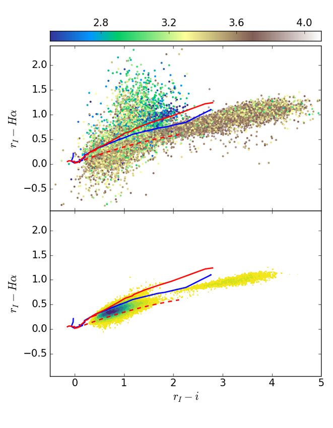
A&A proofs: manuscript no. main

                                                                        ning approximately 0.22 square degrees. The five filters used1 –
                                                                        URGO , g, r, i, Hα – have central wavelengths of 364.0, 484.6,
                                                                        624.0, 774.3, 816.0 nm respectively. Note that the URGO trans-
                                                                        mission curve quite closely resembles that of Sloan u (Doi et al.
                                                                        2010).
                                                                            For UVEX, the sequence of observations at each pointing
                                                                        was r-URGO -g. Before 2012 narrowband HeI 5856 exposures
                                                                        were also included but are not presented here. The exposure time
                                                                        used in each of URGO , g and r was 120, 30, and 30 seconds, re-
                                                                        spectively. For IPHAS the observing sequence was Hα-r-i. The
                                                                        Hα filter exposure time was 120 s throughout. The majority of i
                                                                        and r frames were exposed for 10 s and 30 s respectively. There
                                                                        are two periods of exception to this: in the 2003 observing sea-
Fig. 1. Number of 3-filter exposure sets obtained per year for IPHAS    son, at survey start, the r exposure time was 10 s, while the i
(Hα, r and i, shown in red) and UVEX (r, g and URGO , shown in blue).
                                                                        exposure time was raised to 20 s from 2010 October 29.
                                                                            The northern Galactic plane is covered via 7635 WFC fields
                                                                        that tessellate the footprint with, typically, a small overlap. In ad-
UVEX surveys respectively, and their merger into a single cat-
                                                                        dition, each field is repeated with a shift of +5 arcmin in RA and
alogue recording data on almost 300 million objects. The broad
                                                                        +5 arcmin in Dec in order to fill in the gaps between the CCDs
band calibration is aligned with the Pan-STARRS photometric
                                                                        and also to minimize the effects of bad pixels and cosmic rays.
scale set by Magnier et al. (2013), while the Hα narrow band
                                                                        We refer to each pointing and its offset as a "field pair". Qual-
needs its own bespoke solution. The final catalogue also benefits
                                                                        ity checks were developed and applied to all the data, and those
from a recalculation of the astrometry to place it into the Gaia
                                                                        exposure sets (r, i and Hα – or URGO , g and r) rated as below
DR2 astrometric reference frame. We note that in the case of
                                                                        standard were requeued for re-observation. The ID for each sur-
IPHAS there have been two previous data releases (González-
                                                                        vey pointing is constructed using four digits, starting by 0001
Solares et al. 2008; Barentsen et al. 2014). The last observa-
                                                                        and rising with Right Ascension up to 7635, with an "o" straight
tions were UVEX exposures gathered in late 2018, bringing to
                                                                        after in the case of an offset pointing making up the field pair.
an end a campaign on the INT that began with the first IPHAS
observations in 2003. The new acronym we adopt to represent                 For a plot showing the footprint occupied by both surveys,
the merged database is IGAPS, standing for "The INT Galactic            the reader is referred to figure 2 presented by Barentsen et al.
Plane Survey".                                                          (2014). The difference now is that IPHAS observations are com-
                                                                        plete, filling the whole region between the boundaries at −5◦ <
    Here we summarise the observing strategy, data pipelining           b < +5◦ , 30◦ < ` < 215◦ . For UVEX, the coverage stops just
and quality control shared between the two surveys in sections          short near the celestial equator, at RA = 110◦.0, creating a trian-
2 and 3. The way in which the astrometry is refitted in order           gular region of ∼33 sq.deg. (1.8% of footprint) in which there
to convert it from a 2MASS frame to that of Gaia DR2 is de-             is gradually reducing UVEX coverage of Galactic longitudes
scribed in section 4. After this we turn to the global calibration      greater than ` ∼ 205◦ .
of the UVEX g and r data alongside the r, i, and narrow-band
Hα data of the IPHAS survey (section 5). All surveys have un-
wanted artefacts to deal with and we identify them and their mit-       3. Data reduction and quality control
igation in section 6. Sections 7 and 8 describe the compilation
of the photometric catalogue and its contents. Section 8 includes       3.1. Initial pipeline processing
a comparison between IGAPS source counts and those of Gaia
                                                                        Over the 15 years of data taking, the observations passed from
DR2 and Pan-STARRS. There is also a brief discussion of the
                                                                        the INT to the Cambridge Astronomical Survey Unit (CASU)
4 photometric colour-colour diagrams the catalogue supports. In
                                                                        for processing. A description of the pipeline and its conventions
section 9, we report on a new selection of candidate emission
                                                                        was given in the IPHAS DR2 paper (Barentsen et al. 2014). Fea-
line stars (based on the r − Hα versus r − i diagram: see Witham
                                                                        tures specific to UVEX pipeline processing were noted by Groot
et al. 2008), and on the identification of stellar variables via the
                                                                        et al. (2009). For present purposes it is important to note that the
two epochs of r observation contained within the catalogue. Sec-
                                                                        pipeline (i) produces a photometric calibration based on nightly
tion 10 contains closing remarks.
                                                                        standards referred to a ‘run’ mean, where a run is typically a
                                                                        period of a week or two of observing, (ii) places the astrome-
                                                                        try onto the same reference frame as the 2MASS NIR survey. In
2. Observations and sky coverage                                        producing the IGAPS catalogue, a uniform calibration has been
                                                                        applied and the astrometry has been recomputed to place it in the
The survey observations were all obtained using the Wide Field          Gaia DR2 frame (Gaia Collaboration et al. 2018). See details in
Camera (WFC) mounted on the INT. IPHAS observations began               sections 5 and 4, respectively.
in 2003, while the blue UVEX data gathering began in 2006.
Most of the footprint had been covered once by the end of 2012,
while the later observations mainly focused on repeats correcting       3.2. Quality control
for poor weather and other problems identified in quality control
                                                                        Since the observations were collected over more than a decade
(see figure 1).
                                                                        using a common-user facility, a broad range in observing condi-
    Table 1 provides an overview of key features of the merged          tions necessarily exists within the survey databases. A variety of
IGAPS survey.                                                           quality checks have been developed and applied to all fields as
    The WFC is a 4-CCD mosaic arranged in an L shape with
                                                                        1
a pixel size of 0.33 arcsec/pixel, and a total field of view span-          see http://catserver.ing.iac.es/filter/list.php?instrument=WFC

Article number, page 2 of 28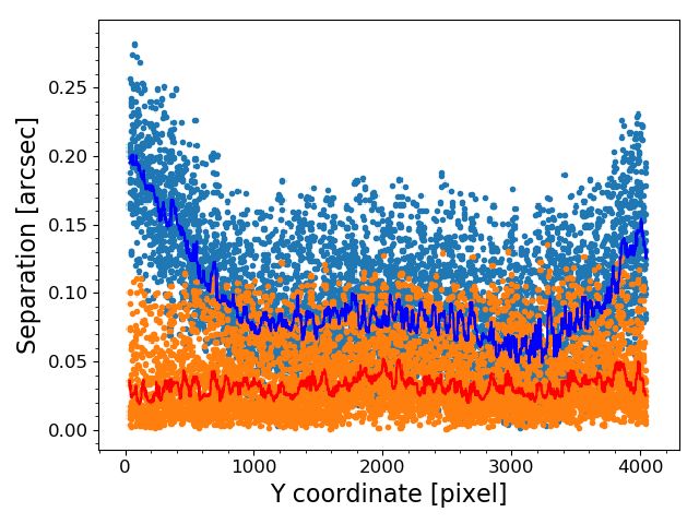
M. Monguió et al.: IGAPS

 Property                                     Value                                                 Comment
 Telescope                                    2.5-m Isaac Newton Telescope (INT)
 Instrument                                   Wide Field Camera (WFC)
 Detectors                                    Four 2048×4100 pixel CCDs
 Pixel Scale                                  0.33 arcsec pixel−1
 Filters                                      i, Hα, r, g, URGO                                     2 r epochs available
 Magnitude System                             Vega                                                  mAB provided as alternative
 Exposure times (seconds)                     i:10, Hα :120, r:30, g:30, URGO :120
 Saturation magnitude                         12(i), 12.5(Hα), 13(r), 14(g) 14.5(URGO )
 Limiting magnitude                           20.4(i), 20.5(Hα), 21.5(r), 22.4(g), 21.5(URGO )      median 5σ detection over the noise.
 median PSF FWHM (arcsec)                     1.0(i), 1.2(Hα), 1.1(r), 1.3(g), 1.5(URGO )
 Survey area                                  ∼ 1860 square degrees
 Footprint boundaries                         −5◦ < b < +5◦ , 30◦ < ` < 215◦
 Beginning/end dates of observations          August 2003 – November 2018                           see Figure 1
Table 1. Key properties of the merged IGAPS survey.

                                                                            ally and only kept if considered free of misleading artefacts. The
                                                                            different checks made are outlined below.
                                                                            1. Exposure Depth: In the top panel of figure 2 we can see the
                                                                               5σ magnitude limit distribution for all the exposure sets in-
                                                                               cluded in the data release. The limits are significantly better
                                                                               than 20 –for r and g–, or 19 –for i and Hα. The exposure sets
                                                                               that do not reach these limits are flagged as f ieldGrade = D.
                                                                               We can see that some fields reach magnitude limits of 22 –in
                                                                               r–, 23 –in g–, and 21 –for i and Hα.
                                                                            2. Ellipticity: The aim was that all included exposures would
                                                                               have mean ellipticity smaller than 0.3. Exposures breaching
                                                                               this limit are labelled f ieldGrade = D. Common values for
                                                                               the survey are in the range 0.15 to 0.20.
                                                                            3. Point spread function at full width half-maximum (PSF
                                                                               FWHM): Where possible, fields initially reported with PSF
                                                                               FWHM exceeding 2.5 arcsec were reobserved. As can be
                                                                               seen in the lower panel of figure 2, the great majority of ex-
                                                                               posures return a PSF FWHM between 1 and 1.5 arcsec in r.
                                                                               And there is the expected trend that stellar images sharpen
                                                                               with increasing filter mean wavelength.
                                                                            4. Broad band scatter: Comparison with Pan-STARRS r, g, and
                                                                               i data is central to the uniform calibration. In making these
                                                                               comparisons, the standard deviation of individual-star photo-
                                                                               metric differences about the median offset (std ps) was com-
                                                                               puted. When this scatter in any one of the three filters ex-
                                                                               ceeds 0.08, the IPHAS (or UVEX) f ieldGrade is set to D.
                                                                               High scatter most likely indicates patchy cloud cover or gain
                                                                               problems.
                                                                            5. Hα photometric scatter: Since the narrow band has no coun-
                                                                               terpart in Pan-STARRS, we use the photometric scatter com-
                                                                               puted between the Hα exposures within a field pair to assess
                                                                               their quality. If the fraction of repeated stars exceeding pre-
Fig. 2. Top: Cumulative distribution of the 5σ limiting magnitude across       set thresholds in |∆Hα| lies above the 98% percentile in the
all published survey fields for each of the five filters. Bottom: Cumula-      distribution of all Hα field pairs, both exposure sets involved
tive distribution of the PSF FWHM for all fields included in the re-           are flagged as f ieldGrade = D. Again, extreme behaviour
lease, measured in the six filters. The PSF FWHM measures the effec-
                                                                               most likely indicates patchy cloud cover or gain problems.
tive image resolution that arises from the combination of atmospheric
and dome seeing, and tracking accuracy.
                                                                            6. Visual examination: Sets of images per field were individu-
                                                                               ally reviewed by survey consortium members. A systematic
                                                                               by-eye examination of colour-magnitude and colour-colour
                                                                               diagrams was also carried out. When severe issues were re-
                                                                               ported, such as unexpectedly few stars, signs of patchy cloud
observed in both surveys. These checks were also used to assign                cover, or pronounced read-out noise patterns, the exposure
a quality flag (or f ieldGrade) from A to D to each field. See table           set would be rejected or given a f ieldGrade = D (if marginal
A for details on how this is implemented. The fields graded as D               and without an alternative).
were rejected and the three filters re-observed when possible. In           7. Requirement for contemporaneous (3-filter) exposure sets:
the absence of replacement, such fields were appraised individu-               The survey strategies required the three IPHAS, or UVEX,
                                                                                                                   Article number, page 3 of 28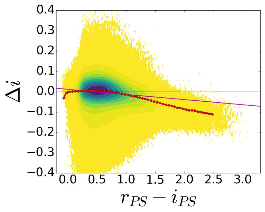
A&A proofs: manuscript no. main

    filters at each pointing should be observed consecutively –       randomly adjusted by up to 5% from the original pipeline solu-
    usually within an elapsed time of ∼5 min. All included ex-        tion values. For the URGO filter PV2_5 is treated in the same way
    posure sets meet this criterion.                                  as PV2_3.
                                                                           The best solution among the 10 tries is found as follows.
                                                                      The separation in arcseconds between IGAPS and Gaia is binned
4. Astrometry: resetting to the Gaia DR2 reference                    with bin sizes of up to 51 stars, depending on the number of stars
                                                                      on the CCD, along the longer axis of the CCD and the median
   frame                                                              in each bin is calculated (solid blue and red lines in figure 3).
The pipeline for the extraction of the survey data, as described in   The solution that has the lowest maximum bin celestial position
previous releases of IPHAS (González-Solares et al. 2008; Bar-        difference is kept as the best astrometric solution. The median of
entsen et al. 2014), sets the astrometric solutions using 2MASS       all bins is kept as the astrometric error to be reported in the final
(Skrutskie et al. 2006) as the reference. This was the best choice    IGAPS catalogue (column posErr).
available at the start of survey observations. Especially for very         The left hand panel of figure 3 shows an example of an ini-
dense fields, source confusion can lead to a wrong world coordi-      tial pipeline and a final astrometric solution. The maximum bin
nate system (WCS) in the pipeline reduced images. Also for the        celestial position difference relative to the Gaia frame in r – the
blue bands in UVEX, particularly the URGO filter, the use of an       filter that provides the position for the great majority of sources
IR survey as the astrometric reference can be problematic.            in the final catalogue – in this example was reduced from 0.23
     The natural choice for astrometric reference now is the Gaia     arcsec initially to 0.061 arcsec in the refined solution. The right
DR2 (Gaia Collaboration et al. 2018; Lindegren et al. 2018) ref-      hand panel of figure 3 shows that the performance in CCD 4,
erence frame. The starting point for a refinement of the astrome-     where the optical axis of the camera falls, is generally to achieve
try is the 2MASS-based per-CCD solution. The pipeline uses the        median position differences under 0.1 arcsec. It also illustrates
zenithal polynomial projection (ZPN, see Calabretta & Greisen         the point that the solutions for URGO are least tight. Experiments
2002) to map pixels to celestial coordinates. In this solution all    with the data suggest the main contribution to the error budget is
even polynomial coefficients are set to 0, while the first order      due to the optical properties of the URGO filter as a liquid filter,
term (PV2_1) is set to 1 and the third order term (PV2_3) to 220.     with differential chromatic refraction playing only a minor role.
Occasionally, it was found that for the URGO filter a fifth order     However the improvement this represents for URGO is arguably
term (PV2_5) also needed to be introduced. Free parameters in         greater than for the other filters, in that the original astrometry
the solution were the elements of the CD matrix, which is used        was often so poor that cross-matching of this filter to the others
to transform pixel coordinates into projection plane coordinates,     would fail for much of the camera footprint. In this respect, a
and the celestial coordinates of the reference point (CRVALn).        recalculation of the astrometry was a pre-requisite for the suc-
     For the refinement of the astrometric solution using the Gaia    cessful construction of the IGAPS catalogue.
DR2 catalogue we first remove IGAPS stars that are located
close to the CCD border. We also remove very faint stars. The
limit for removal is set as a threshold on the peak source height:    5. Global photometric calibration
the value chosen depends on the number of sources in the image,
varying between 20 (in low stellar density fields) and 150 (high      The approach to global calibration is as follows. Since the en-
density fields) ADU. An exception is made for the URGO filter         tire IGAPS footprint falls within that of the Pan-STARRS survey
where the threshold is always 10 ADU. Next, we search for Gaia        (Chambers et al. 2016), we have chosen to tie IGAPS g, r, and i
DR2 sources within a 0.5 degree radius of the field centre. We        – the photometric bands in common – to the Pan-STARRS scale
then remove all sources that have a proper motion error in either     (Magnier et al. 2016). By doing this it is possible to piggy-back
Declination or Right Ascension greater than 3 mas/yr. The Gaia        on the high quality ’Ubercal’ that benefitted particularly from the
catalogue is then converted to the IGAPS observation epoch us-        much larger 3-sq.deg. field of view of the Pan-STARRS instru-
ing the stilts Gaia commands epochProp and epochPropErr               ment (Magnier et al. 2013). With the g, r, i calibration in place,
(Taylor 2006).                                                        we are then able to link in the narrowband Hα, as described be-
     The Gaia and the IGAPS catalogues are then matched us-           low. A global calibration of URGO is not attempted at this time
ing the match_coordinates_sky function in the astropy package         (see Section 8.6 for more comment).
(Astropy Collaboration et al. 2013; Price-Whelan et al. 2018).             Previous IPHAS data releases have provided photometry
Matches with a distance larger than 1.5 arcseconds are removed        adopting the Vega zero-magnitude scale. We continue to do this
as spurious. Hence the initial astrometric solution of the pipeline   here, whilst also offering the option in the catalogue of magni-
needs to be better than this - which it usually is - if the search    tudes in the (Pan-STARRS) AB system.
for a refined solution is going to succeed. In the rare cases where
the pipeline solution is worse than this, a good enough initial       5.1. Calibration of g, r and i, with respect to Pan-STARRS
astrometric solution needs to be found by hand.
     As the ZPN projection cannot be inverted, its coefficients       The calibration was carried out on a chip by chip basis, comput-
need to be found iteratively. We are using the Python package         ing the median differences between IGAPS and Pan-STARRS
lmfit (Newville et al. 2014) with the default Levenberg Marquart      magnitudes in each of the three filters, after allowing for a colour
algorithm for finding the iterative solution. The fitting function    term as needed. In order to compute these, we plotted the differ-
converts the IGAPS pixel positions into celestial coordinates         ences in magnitude as a function of colour, paying attention to
using the ZPN parameters and calculates the separation to the         sky location. Specifically, we computed the shift gradient as a
matched Gaia source, which is minimized. As the solution de-          function of colour for a set of boxes spanning the survey foot-
pends on the initial parameters, we run the algorithm with 10         print. No significant trend was apparent in any filter, although
different starting parameter sets: the original pipeline solution;    variation in the gradient by up to ±0.01 was noted. We provide
the set of median coefficients for the CDn_m and PV2_3 values         an example of the colour behaviour for each of the filters in fig-
of the filter; plus 8 sets where CRPIXn, CDn_m and PV2_3 are          ure 4. We concluded that, overall, there is no need for a colour
Article number, page 4 of 28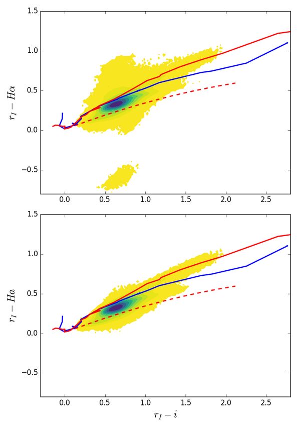
M. Monguió et al.: IGAPS

Fig. 3. Left: Celestial position difference between the IGAPS catalogue and Gaia DR2 stars on CCD#1 of INT image r908084. The original
pipeline solution is shown in cyan and the refined solution in orange. The binned median curves are shown in blue and red, respectively. Right:
Histogram of the median celestial position difference for WFC CCD#4 between IGAPS and Gaia DR2 by filter. The r filter (orange) includes
IPHAS and UVEX data. The median differences are: 72 (URGO ), 39 (g), 38 (r), 46 (Hα) and 45 (i) mas.

                                                                               The ranges used were 15 < g < 19, 14.5 < r < 18.5, and
                                                                               13.5 < i < 17.5 mag.
                                                                                    Once the shift for each CCD and filter is computed, the cal-
                                                                               ibrated AB magnitude for each star is recovered. This proceeds
                                                                               by first calculating the corrected r magnitude in the AB system,
                                                                               via:

                                                                               rAB = r p + 0.125 − ∆ZPr                                          (2)

                                                                               The ground is then prepared for finding the gAB and iAB magni-
                                                                               tudes taking into account the relevant colour term:

                                                                                          1      h                                 i
                                                                               gAB =            · g p − 0.110 − ∆ZPg + 0.040 · rAB
                                                                                        1.040                                                    (3)
                                                                                          1
                                                                                      =         · i p + 0.368 − ∆ZPi + 0.060 · rAB

                                                                                iAB
                                                                                        1.060

Fig. 4. Differences between IGAPS and Pan-STARRS magnitudes -                  Then, finally, the Vega corrected magnitudes are computed from
after taking out the raw per CCD median shift- vs Pan-STARRS colour.           these AB alternates using the shifts appropriate in the Pan-
Data from the range 50◦ < ` < 70◦ , −5◦ < b < +5◦ are shown. Top-              STARRS filter system:
left: ∆g vs (g − r), top-right: ∆rU vs (g − r), bottom-left: ∆rI vs (r − i),
bottom-right: ∆i vs (r − i). Only stars with 14 < g ps < 20, 13 < r ps < 19
or 12.5 < i ps < 18.5 are used in these plots. The magenta line is the         r = rAB − 0.121
fitting line. The red dots follow the running median for each 0.05 mag         g = gAB + 0.110                                                   (4)
bin showing where the trends deviate. The false colour scale indicates         i = iAB − 0.344
density of sources in each bin on a square root scale with yellow rep-
resenting the lowest density of at least 4 sources per 0.02x0.02 mag2
bin.                                                                           An example of this calibration step operating in one 5x5 sq.deg.
                                                                               box is shown in the first two panels of figure 5.
term in handling the r band, whilst correction is appropriate for                   For faint red stars, when an i magnitude is available but not
g and i.                                                                       r, the final i magnitude is computed without taking into account
    The final calibration shifts applied per band per CCD are:                 the colour term. In such a case, the photometric error is raised
                                                                               to acknowledge this by adding in 0.05 mag, in quadrature. The
∆ZPr = median(r p + 0.125 − rPS )                                              same remedy is adopted for the much rarer instances of blue/faint
∆ZPg = median (g p − 0.110 − gPS ) − 0.040 · (gPS − rPS ) (1)                  objects for which g is available but not r.


∆ZPi = median (i + 0.368 − iPS ) + 0.060 · (rPS − iPS )
               p                                                                  The standard deviation of the differences relative to Pan-
                                                                               STARRS for each CCD chip (std ps), computed alongside the
where the superscript p indicates the Vega magnitudes from the                 median shift (equation 1) is retained to serve as a measure of the
pipeline and the constants in the first right-hand-side brackets               quality of the IGAPS photometry. For example, a photometric
are the transformation coefficients from Vega to AB magnitudes                 gradient across a chip, due to cloud or a focus change, will not be
in the INT filter system. To assure the quality of the shift cal-              removed by the calibration shift, but will increase the recorded
culation, only those stars within a specified magnitude range                  standard deviation. This datum is used within the seaming pro-
were taken into account, in order to avoid bright stars subject to             cess in deciding which detections to identify as primary in the
saturation, and fainter objects with relatively noisy magnitudes.              final source catalogue.
                                                                                                                         Article number, page 5 of 28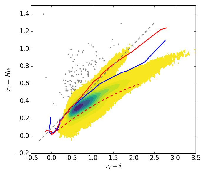
A&A proofs: manuscript no. main

Fig. 5. 5x5deg2 box at 170◦
M. Monguió et al.: IGAPS
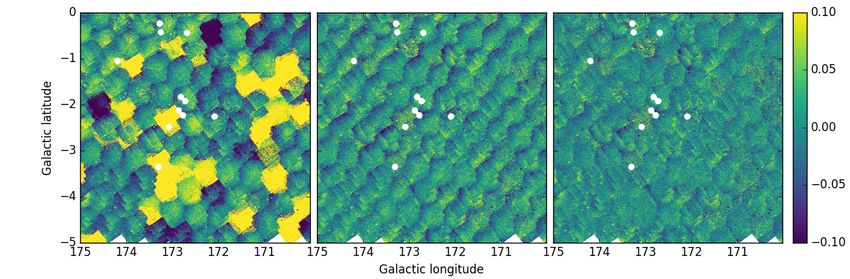
Fig. 7. To illustrate the outcome of the Hα calibration, the Galactic Plane footprint is shown with all the fields marked as points. Colour indicates
the shift applied to the Hα zeropoint, according to the Glazebrook correction, while the black squares indicate the fields used as anchors.
into account, as precise measurements of them were not avail-
able and they are expected to be grey over the r-band filter.
The different versions of the CALSPEC Vega spectrum intro-
duce only a small change of 0.003 mag in the offset calculation.
A similar change can be achieved by using different measure-
ments of the filter curves obtained over the survey years at the
ING. The effect of airmass is a lowering of about 0.003 mag per
0.1 airmass change over the range that survey observations were
taken. Finally an increase of about 0.0025 mag per 5 mm PWV
is found. The Hα zeropoint offset from r found this way is 3.137.
However, when comparing synthetic stellar locations to the data
it was found that the location of A0 dwarf stars is not at zero
colour in r-Hα, as would be expected by definition in the Vega
system. The cause of this lies in a unique aspect of the standard
star Vega, namely it being a fast rotator viewed nearly pole on
(Hill et al. 2010), which introduces a difference in the Hα line
profile when compared to other A0 dwarf stars. Indeed, the other
CALSPEC A0V standards, HD116405 and HD180609, show a
lower value of the zero point offset between r and Hα. The value
we used for the offset is the average of the offsets derived from
these two stars with the different filter profiles measured over the
years. Using this value of 3.115 for the zeropoint offset between
r and Hα is equivalent to saying that the magnitude of Vega in
the Hα filter is 0.022 mag fainter than in the broadband filters.
To deal with random shifts due to poor and variable weather,
a second correction is applied that seeks to minimize the differ-
ences between Hα magnitudes –after illumination correction is
applied – in the zones of overlap between fields (Glazebrook
Fig. 8. r − Hα vs r − i diagrams for the region 165◦ < l < 170◦ be-
et al. 1994). This requires the selection of the best fields, or
fore (top) and after (bottom) the Glazebrook calibration, using sources
with rI < 19 and errBits=0. Lines indicate the expected sequences: anchors, that are fixed under the assumption their photometry
unreddened main sequence in red, giants sequence in blue, and redden- needs no further correction. The fields to be used as anchors are
ing line for an A2V star up to AV =10 in dashed red. See Appendix D carefully selected taking into account: the standard deviation of
for photometric colour tables. As explained by Drew et al. (2005) and the magnitude differences with Pan-STARRS (std ps) in r and
Sale et al. (2009), the elongation of the main stellar locus is due to the i, to avoid magnitude gradients in the field; the number of stars
combined effects of interstellar extinction and intrinsic colour. The false crossmatched with the Pan-STARRS catalogue, to ensure ade-
colour scale indicates density of sources in each bin on a square root quate statistics; the median value of the magnitude differences
scale with yellow representing the lowest density of at least 4 sources between the field and its offset pair, taken to indicate a stable
per 0.02x0.02 mag2 bin. night. As a final precaution, the (Hα − r) vs. (r − i) diagram for
each potential anchor field was inspected to check for consistent
placement of the main stellar locus. The shifts applied and the
(similar altitude to La Palma), an airmass of 1.2 (as used by Pan- selection of anchors can be seen in figure 7. In figure 8 we can
STARRS, Tonry et al. 2012, and close to our survey median of see the r − i vs r − Hα diagrams for the region 165◦ < l < 170◦
1.15) and a precipitable water vapour (PWV) content of 5 mm before and after the Glazebrook calibration – the improvement
(García-Lorenzo et al. 2009). Optical surfaces were not taken is clear.
Article number, page 7 of 28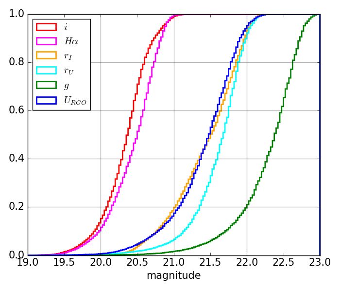
A&A proofs: manuscript no. main

                               Filter           h fλ i           EW         λ0       λp        Vega magnitude
                                        (erg cm−2 s−1 ) Å−1      (Å)       (Å)      (Å)      AB      Vega system
                               URGO         4.24 × 10⁻⁹         138.8     3646     3640     0.742       0.023
                                 g          4.98 × 10⁻⁹         716.7     4874     4860     −0.088      0.023
                                 r          2.44 × 10⁻⁹         745.3     6224     6212     0.153       0.023
                                Hα          1.79 × 10⁻⁹         57.1      6568     6568     0.373       0.045
                                 i          1.29 × 10⁻⁹         708.2     7677     7664     0.393       0.023
Table 2. As table 2 in Barentsen et al. (2014) with values for all the survey filters. Mean monochromatic flux of Vega, filter equivalent width, mean
photon and pivot wavelengths as defined in Bessell & Murphy (2012) are given, along with the calculated AB and defined Vega system magnitudes
for the CALSPEC Vega spectrum stis_009 (the Vega broad band magnitude is from Bohlin 2007). Note that the catalogue data for URGO is not
globally calibrated and the broad band filters g, r and i are transformed onto the Pan-STARRS photometric system.

6. Artefact mitigation                                                      tortion would not be tracked adequately and would lead to over-
                                                                            large aperture corrections in the affected area of the chip.
With astrometry re-aligned to the Gaia DR2 reference frame, and                  After mapping the regions affected (and the variations as a
a uniform calibration in place, the next steps are to conduct some
                                                                            function of date of observation, due to rotation of the filter within
final cleaning and flagging.
                                                                            its holder from time to time), we are able to flag the stars falling
                                                                            in them. This is done at two levels of impact. We have defined as
6.1. Mitigation of satellite trails and other linear artefacts              the inner, most severely affected region within the camera foot-
                                                                            print, those locations where the photometric discrepancy exceeds
The night sky is criss-crossed by satellites and meteors liable to          0.1 mag, while the threshold set for the outer region is 0.05 mag.
leave bright trails in exposed survey images, essentially at ran-           The lower of these thresholds corresponds to roughly 4 times
dom. It is far and away most common that the photometry of                  the median shift elsewhere in the footprint (computed for stars
any given detected object is adversely affected in one band only            in the range 15 < g < 19). The g-band detections masked in this
by this unwanted extra light. Nevertheless, it is important to the          way always fall near the edge of the imaged area, within an area
value of the final merged catalogue that instances of the problem           amounting to roughly 0.07 of the total. In terms of primary de-
are brought to the user’s attention.                                        tections listed in the catalogue, the choices made in the seaming
    To achieve this, we have visually inspected composite                   algorithm bring the g-mask flagged fraction down to 0.015. More
plots of IPHAS-bands and UVEX-band catalogued objects, not-                 detail on how the g mask is imposed is given in supplementary
ing instances of trails and other linear artefacts. The affected            materials (Appendix B).
individual-filter flux tables are then visited in order to mark and
flag these features. Satellite trails usually show up very easily           6.3. Bright stars, ghosts and read-out problems
in these plots. But, in more ambiguous cases, the images them-
selves have also been checked. Strips of width 30 pixels – have             Bright stars can affect the photometry of other stars nearby. Not
been computed and placed on all noted linear streaks, and have              only that, but features in e.g. the diffraction spikes are sometimes
been used to flag all sources falling within them as at risk. This          picked up as sources by the pipeline. To support screening these
intensive visual inspection also brought to the fore other linear           out, we have identified all the stars in the Bright Star Catalogue
structures such as spikes due to bright stars, crosstalk, and read-         (Hoffleit & Jaschek 1991) that are brighter than V = 7 in the sur-
out problems and meant they too could be flagged.                           vey area and have flagged all catalogued sources that lie within a
                                                                            radius of 5 arcmin of any of them. For sources brighter than 4th
                                                                            magnitude, this radius is raised to 10 arcmin. Clearly some real
6.2. Masking of localised PSF distortion on the g-band filter
                                                                            sources that happen to be close to bright stars will be caught up
With the accumulation of more and more survey data and the                  in this, and flagged. Interested users of the catalogue are encour-
release of Pan-STARRS data (Chambers et al. 2016), it became                aged to check the images (when available) in these instances, re-
possible to co-add large numbers of detected-source magnitude               membering that the background level is higher in these flagged
offsets referred to pixel position in the image plane. This reveals         regions with the result that sources in them may not be as well
any localised variations in photometric performance that might              background-subtracted as sources in the wider unaffected field.
otherwise be missed. In the case of the g band, this procedure                  Bright stars outside the field can also create spikes due to
revealed a clear distortion towards the edge of the image plane             reflections in the telescope optics. When linear, these will have
compromising the extracted photometry. Subsequent visual in-                been flagged as part of the procedure described above in sec-
spection of the filter by observatory staff confirmed the presence          tion 6.1. But occasional, more complex structures are likely to
of a blemish near its edge, in the right place to be linked with the        be missed. In this category we place the structured dominantly-
evident photometric distortion.                                             circular ghosts of stars brighter than V = 4. These are obvious
    Since flat field frames taken through the g filter did not be-          in the processed images and also show up as rings in wider-area
tray the problem, a transmission change could not be implicated.            plots of catalogued objects.
Instead a change in the character of the point-spread function                  As the Wide Field Camera aged during the execution of
(PSF) had to be involved. Further checking revealed that point-             IPHAS and UVEX, electronic glitches during read-out – creat-
source morphologies returned by the extraction pipeline were                ing jumps in the background level – became progressively more
changing (sharpening) in the region of the blemish. Since the               frequent. In cases where the whole image is affected by tell-tale
PSF and associated aperture corrections are computed in the                 strips and lines, it is discarded. But sometimes this issue affects
pipeline per CCD, these changes over the smaller area of dis-               just a small portion of one CCD. In cases like this, the image is
Article number, page 8 of 28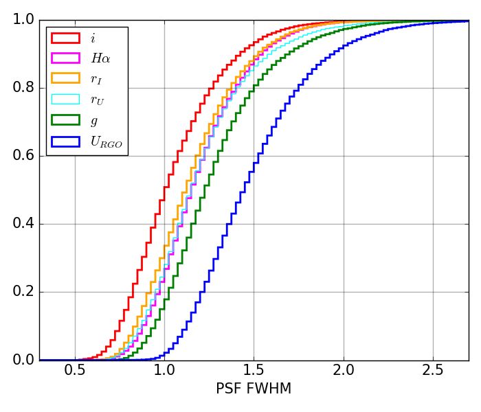
M. Monguió et al.: IGAPS

            Star            RA             DEC                `            b       V      IDs of affected fields
            Capella     05 16 41.36     +45 59 52.77       162.589       +4.566   0.08    2298, 2298o
            Deneb       20 41 25.92     +45 16 49.22        84.285       +1.998   1.25    6116, 6116o, 6083o,6093
            Elnath      05 26 17.51     +28 36 26.83       177.994       -3.745   1.65    2416,2416o,2452,2452o
            Alhena      06 37 42.71     +16 23 57.41       196.774       +4.453   1.92    3720,3720o,3690,3690o
            γ Cyg       20 22 13.70     +40 15 24.04        78.149        1.867   2.23    5868,5868o,5831,5831o,5855,5855o
            β Cas       00 09 10.69     +59 08 59.21       117.528       -3.278   2.27    0043,0043o,0052,0052o,0066
            γ Cas       00 56 42.53     +60 43 00.27       123.577       -2.148   2.39    0324,0302,0302o,0296,0296o
            δ Cas       01 25 48.95     +60 14 07.02       127.190       -2.352   2.68    0459o,0475o,0477,0477o
            µ Gem       06 22 57.63     +22 30 48.90       189.727        4.169   2.87    3413,3413o,3428
            γ Per       03 04 47.79     +53 30 23.17       142.067       -4.337   2.93    1051o,1055,1055o
            ζ Aql       19 05 24.61     +13 51 48.52        46.854       +3.245   2.99    4483,4483o
             Aur       05 01 58.13     +43 49 23.87       162.788       +1.179   2.99    2084,2084o,2106,2106o,2119
Table 3. Stars brighter than V = 3 mag. located within the IGAPS footprint. It is recommended that catalogue users seeking photometry in
the vicinity of these objects, especially, should check images (Greimel et al, in prep.) to better understand the likely impact they have on the
photometry. For convenience both celestial and Galactic coordinates are given.

retained if there is no alternative exposure available, while the         those, using the same priority as for the coordinates, i.e. rI , rU ,
sources in the minority problematic regions are flagged.                  i, Hα, and g.
                                                                               For each band we have a flag (mClass) indicating whether
6.4. Saturation level and the brightest stars
                                                                          a source looks like a star (mClass = −1), an extended object
                                                                          (mClass = 1) or noise (mClass = 0). It can also indicate a
Stellar images typically begin to saturate at magnitudes between          probable star (mClass = −2) or a probable extended object
12 and 13. Catalogued objects affected by this are flagged. The           (mClass = −3). A general mergedClass flag will be set up to the
precise saturation magnitude in an exposure is somewhat depen-            same values if the different mClass for all the available bands
dent on the seeing and sky conditions, both of which varied sig-          agree. Otherwise it will be set to 99. From the combination of
nificantly over the 15 years of data gathering.                           these classes, we compute the probability for a source to be a
    It is worth noting that there are some extremely bright stars in      star, noise or an extended source (pS tar, pNoise, pGalaxy).
the footprint that not only saturate but have a major detrimental              Boolean flags are also set up indicating whether the source
effect on the photometry collected from the whole CCD in which            in a given band is affected by deblending, saturation, vignetting,
they are imaged, and more. In the most extreme case of Capella,           trails, truncation for being close to the edge of the ccd, or if it is
nearly the entire 4-CCD mosaic is compromised. Such objects               close to a bad pixel. For each source and band, the user can also
create rings, bright spikes and halos, ghosting between CCDs,             find the ellipticity, the median Julian date of the observation, and
as already mentioned in Section 6.3. In table 3 we list the stars         the seeing.
brighter than V =3 mag in the footprint that are most challenging              As a summary of the information provided by different
in this regard.                                                           bands, some final boolean flags are also available: brightNeighb
                                                                          if the object is located within a radius of 5 arcmin from an source
7. Generation of the source catalogue                                     brighter than V=7 according to the Bright Star Catalogue (Hof-
                                                                          fleit & Jaschek 1991), or within 10 arcmin if the neighbour is
7.1. Catalogue naming conventions and warning flags                       brighter than V = 4, deblend if there is another source nearby,
                                                                          and saturated if it saturates in one of the bands. nBands indi-
The detailed description of columns in the catalogue will be
                                                                          cates the number of bands available for each source from the six
given in Appendix C. Here we explain the meaning for some
                                                                          possible i, Hα, rI , rU , g, URGO . nObsI is the number of IPHAS
of the columns.
                                                                          repeat observations available for this source and nObsU is the
     The name for each source, as suggested by the IAU, is
                                                                          same for UVEX.
uniquely identified by an IAU-style designation of the form
’IGAPS JHHMMSS.ss+DDMMSS.s’, where the name of the                             Another global quality measure provided is errBits. It will
catalogue IGAPS is omitted in the catalogue. The coordinates              be the addition of: 1 if the source has a bright neighbour; 2 if
of the source are also present in decimal degrees and in Galac-           it is a deblend with another source in any band; 4 if it has been
tic coordinates in columns RA, DEC, gal_long, and gal_lat. The            flagged as next to a trail in any band; 8 if it is saturated in any
coordinates come with an error (posErr) computed as indicated             band; 16 if it is in the outer masking of the g band blemish; 64
in Sect. 4. Since each source can be measured in up to six differ-        if the source is vignetted near the corner of CCD 3 in any band;
ent bands, we always use as a reference rI if available. If it is not,    128 if it is in the inner mask of the g band blemish; 256 if it is
then we will use, in order of preference, the coordinates extracted       truncated near the CCD border in any band; 32768 if the source
from the following bands: rU , i, Hα, and g. The differences in as-       sits on a bad pixel (in any band). If ErrBits is not equal to 0, the
trometry between the designated coordinates and the individual            user should exercise care when using the information provided
band coordinates can be found in mDeltaRA and mDeltaDec for               for the source.
each of the filters –except for rI , that it is not included since be-
ing the primary source for the astrometry, it would always be             7.2. Bandmerging and primary detection selection
zero if available. We provide another identifier for each band in
mdetectionID, created by adding the run number of the original            The merging of the different bands involves two steps. First, the
image, the ccd number and the detection number within this ccd,           three contemporaneous bands for each of IPHAS and UVEX are
i.e. ’#run-#ccd-#detection’. A general sourceID is chosen from            merged. We use the tmatch tool within stilts (Taylor 2006) to
                                                                                                                   Article number, page 9 of 28
A&A proofs: manuscript no. main
obtain tables collecting together information on the three bands N (×106 )N (×106 )
for each source, adopting an upper limit on the on-sky cross- errBits=0
match radius of 1 arcsec. With the re-working of the astrometry IGAPS (surveys combined)
into the Gaia DR2 reference frame, it might seem that a tighter All 295.4 205.2
limit of e.g. 0.5 arcsec could be applied. Whilst this is almost al- IPHAS 264.3 186.1
ways true (see Section 8.3), we used the more forgiving 1 arcsec UVEX 245.8 170.7
bound to allow for the optical differences internal to the sepa- IPHAS + UVEX 214.7 151.6
rate filter sets of IPHAS (including Hα narrowband) and UVEX IPHAS
(including URGO ). It also gives more room to keep high proper i, Hα, rI 168.4 115.4
motion counterparts together on merging the IPHAS and UVEX i, rI 31.7 25.2
r observations. Sources missing a detection in one or more fil- i 25.6 18.9
ters are retained in this process, with the columns for the missing Hα 15.7 11.2
band(s) left empty. rI 16.3 12.0
Before the final UVEX-IPHAS merging, we must take into UVEX
account the normal situation that a source in either catalogue has rU , g, URGO 54.3 30.0
typically been detected in a given band more than once. This rU , g 101.1 72.7
arises from the standard observing pattern of obtaining a pair rU 76.2 60.6
of offset exposures for every filter and field (a practice aimed at g 12.7 6.8
eliminating as far as possible the on-sky gaps that would other- Table 4. Number of sources in the catalogue for the stated survey/filter
wise exist due to the WFC’s inter-CCD gaps). To bring to the combinations. The first column of numbers counts all catalogue rows,
fore the best available data, we do not stack information from while the second gives totals for the best quality errbits=0 sources.
repeat measures, but instead select the best measurement per Combinations of filters not shown individually account for less than
source. To do that, we prioritise according to the following rules. 2% of the total number of catalogue rows. The IPHAS part of the table
If there is no clear winner at any one step, we then move to the pays no attention to whether there are any UVEX detections and vice
versa for the UVEX part of the table.
next:
1. Choose detection with greater number of bands available.
2. Reject f ieldGrade=D if other options are available.
Both IPHAS and UVEX photometric data are available for a
3. Choose detection with smallest errBits.
subset of 214.7 × 10⁶ objects. Table 4 provides details on the
4. Pick the detection with the smaller photometric dispersion in
numbers of sources for different combination of filters across the
the Pan-STARRS comparison, using the std ps flag.
two surveys, together and separately. The number of stars rais-
5. Choose best seeing. ing no flags, for which errBits= 0, are also given for each of the
6. Select detection closest to the optical axis of the exposure tabulated combinations.
set. In general terms, sources with detections in several bands
The detection emerging from this process becomes the primary are most likely real. However, there can also be real objects that
detection in the final catalogue. The second best option is also re- are picked up in only one band. For example, very red and faint
tained and made available in the final catalogue with magnitudes sources may have only a detection in i. Or a knot within a re-
labelled with a ’2’, i.e.: i2, Hα2, rI 2, rU 2, etc. as the secondary gion of Hα extended nebulosity, may appear in the catalogue
detection. A subset of the flags describing primary detections as an Hα-only measurement. Broadly speaking, we recommend
are provided for secondary detections also. Not every primary reliance on the various warning flags available, and on the num-
detection is accompanied by a secondary detection. ber of measurements nObsI and nObsU listed, in concluding on
Once two separate catalogues are created, one for IPHAS whether a source is real or spurious. When the user wants to limit
and one for UVEX, with the selected primary and secondary de- a selection to purely the best-quality detections over all avail-
tections in each, the two catalogues are merged, again using the able bands, the appropriate action is to include the requirement,
tmatch tool within stilts. Because stars vary, the cross-matching errbits = 0.
of the two catalogues does not insist on a maximum difference
in r magnitude before accepting – accordingly, acceptance of a
8. Evaluation of the catalogue contents
cross-match is based entirely on the astrometry.
8.1. On photometric error as a function of magnitude
7.3. Compiling the final source list and advice on selection The median photometric errors reported in the catalogue are
shown as a function of magnitude in figure 9. They are assigned
The final catalogue contains 174 columns, as described in the
by the pipeline on the basis of the expected Poissonian noise
Appendix C. In order to try to minimise spurious sources, we
in the aperture photometry. In order to estimate the scale of the
enforce two further cuts on the final catalogue:
errors associated with their reproducibility (in effect, a scatter
1. Objects with measurements in only the URGO band are not about the mean Pan-STARRS reference), we also plot in figure 9
included. the absolute median magnitude difference between each primary
2. A source should have a detection limit of S/N>5 in at least detection and its corresponding secondary. We note that the sec-
one of the other bands: i.e. it is required that at least one of ondary detection will, by definition, be lower quality in some
iErr, haErr, rErrI , rErrU or gErr is smaller than 0.2 mag. aspect than the primary, and that the total number of measures
available is smaller than the total number of primary detections
This leads to a final catalogue of 295.4×10⁶ rows, each asso- because not every primary has a secondary. The error bars on
ciated with a unique sky position. This splits into 264.3/245.8 × both measures indicate the 16 and 84 percentiles of the errors
106 rows in which IPHAS/UVEX measurements are provided. for all the sources in a given 0.5 mag bin.
Article number, page 10 of 28M. Monguió et al.: IGAPS
The effect of saturation is clear to see at the bright end in
figure 9 for the most sensitive r and g filters. Essentially the pho-
tometry worsens noticeably relative to results at fainter magni-
tudes at r < 12.5 and g < 13.0. The very best photometry is
achieved between 13.0 and 18-19 mag, depending on filter. In
this range, reproducibility rather than random error dominates.
In all filters except URGO , the median error level is at or below
0.02, and shows more scatter than implied by the pipepline ran-
dom error. This level has been drawn into figure 9 to aid the eye.
In r it is between 0.015 and 0.02. Factors contributing to the re-
producibility error would include a mix of real data effects (e.g.
focus gradients within the CCD footprint), and imprecisions in
the data processing (e.g. the dispersion around the adjustment of
the illumination correction, known to be σ=0.008 – see section
5.2).
At faint magnitudes (>20th), the median primary-secondary
differences are comparable with and can sometimes be lower
than the Poissonian error. The greater dispersion of the errors
in URGO band reflects at least in part the fact this band is not yet
uniformly calibrated.
8.2. On the numbers of sources by band and Galactic
longitude
Previous works based on the IPHAS survey alone have already
investigated how the density of source detections in the r, i
and Hα bands depends on Galactic longitude (González-Solares
et al. 2008; Barentsen et al. 2014; Farnhill et al. 2016). Of par-
ticular note in this regard is the study by Farnhill et al. (2016)
which also looks at completeness in the r and i bands. Here, we
bring the added UVEX filters into view.
Figure 10 shows the latitude-averaged density of all cata-
logued objects as a function of Galactic longitude for each of
the six survey bands, subject to the requirement that a good de-
tection in the i band is available at a magnitude less than 20.5
(the median 5σ limit - see figure 2). The effect of extinction is
clear to see in that, in the first Galactic quadrant, even the r stel-
lar densities are a little lower than in i. The limiting magnitudes
of the Hα and i data are much the same, and so the Hα detection
density is noticeably lower when extinction is more significant.
At all longitudes, the density of URGO detected objects is be-
tween ∼ 10 and ∼20 thousand per sq.deg. (∼ 4 per sq.arcmin.).
It is worth noting that, where i < 18, the detection rate in g, r
and Hα relative to i band is close to 100%, and ∼50% or better
in URGO : as i increases above 18, there is a progressive peeling
away until the position shown in figure 10 is reached. In the sec-
ond Galactic quadrant, there is good and quite even coverage in
all bands (with URGO at ∼ 40%, all the way down to i ∼ 20 mag.
The decrease in source density for the UVEX bands at Galac-
tic longitude ∼210◦ reflects the missing UVEX coverage in the
corner of the footprint (see section 2).
8.3. On internal astrometric accuracy
As described in section 7.2 the cross match between bands was
done in two steps, with a 1 arcsec radius. In table 5 we provide
data on how this works out in practice: we compare the differ-
ences in astrometry between bands, based on the mDeltaRA and
mDeltaDEC catalogue columns for each band. We provide the
Fig. 9. In black, median photometric errors for 0.5 mag bins for each median and 99 percentile separations for stars up to rA&A proofs: manuscript no. main
Fig. 10. Number of sources as a function of Galactic longitude in each of the six pass bands, subject to the following requirements: i < 20.5 mag;
the i PSF is star-like (iClass < 0); errbits < 2 (see section 7.3).
r < 20 All sources at ` = 60◦ than at ` = 100◦ , where there is undoubtedly more
percentiles 50% 99% 50% 99% crowding. If the Gaia sources left unpaired by the initial match
rI vs i 0.04 0.36 0.06 0.43 are cross-matched a second time with the IGAPS catalogue, then
rI vs Hα 0.04 0.38 0.06 0.45 9693/25286 at ` = 60◦ and 2156/5250 at ` = 100◦ find partners
rI vs rU 0.05 0.34 0.07 0.47 (already partnered in the first round) – a ∼40% success rate. This
rU vs g 0.04 0.36 0.06 0.43 behaviour shows that the much sharper Gaia PSF resolves more
rU vs URGO 0.10 0.48 0.10 0.48 sources at faint magnitudes. At ` = 60◦ we have a density in the
Table 5. Median and 99 percentile for the source position differences region of 300 000 sources/sq.deg. At a a typical IGAPS seeing
between bands. Units in arcseconds. of 1-1.2 00 (see figure 2), this leads to a ∼1/11 source per beam,
well above the rule-of-thumb 1/30 confusion limit mentioned by
Hogg (2001). At ` = 100◦ the source density is lower by a factor
fit to the Gaia DR2 frame presented in section 4. The same is of 2, roughly.
true for the contemporaneous UVEX rU vs g separations. The We have checked the quality flags for the sources found in
cross match between the IPHAS and UVEX fields using the IGAPS but not in Gaia to reject the hypothesis that they are just
non-contemporaneous astrometry for the rI and rU bands gives noise. 80% of the sources not found in Gaia have ErrBits=0
slightly larger median values, but it is still the case that separa- making it unlikely they are spurious sources. Note that in fig-
tions as large as 0.5 arcsec are extremely rare. The greatest dif- ure 11 we have as x axis both IGAPS r and Gaia G magnitudes,
ference is encountered when the URGO filter is involved. The me- which despite being very similar for modest r − i, have a grow-
dian rU to URGO separation of 0.1 arcsec is nevertheless broadly ing colour dependence for increasing r − i, as can be seen in fig-
compatible with the residuals of the astrometry refit (cf. the bot- ure 12. A minor factor in figure 11 is that IGAPS sources might
tom row of table 5 with the right panel of figure 3). not have a measured r magnitude (either rI or rU ), and so could
not be included.
In the same two 1 sq.deg. areas, we have compared the
8.4. Comparison with Gaia and Pan-STARRS IGAPS catalogue with Pan-STARRS (Chambers et al. 2016). In
In order to compare our catalogue depth and completeness we this case there are more sources in the Pan-STARRS catalogue.
have developed a simple unfiltered cross match with the Gaia In figure 13 we can see that Pan-STARRS is a bit deeper in the
DR2 catalogue (Gaia Collaboration et al. 2018) in two 1 sq.deg. r band, but not by much. In this figure we are directly compar-
regions. The first is a high stellar density region: 60◦ < ` < 61◦ , ing Pan-STARRS and IGAPS AB magnitudes that are the same
0◦ < bM. Monguió et al.: IGAPS
Fig. 13. Results of the crossmatch between IGAPS and Pan-STARRS at
` = 60◦ . In blue, rAB magnitude distribution for the IGAPS sources. In
red, r magnitude distribution from Pan-STARRS. In green, sources with
both IGAPS and Pan-STARRS values. In cyan, sources in IGAPS not
crossmatched with Pan-STARRS. In orange, sources in Pan-STARRS
but not in IGAPS. When two r magnitudes are available for an IGAPS
source (rABI and rABU ), then mean value is plotted, in a way that when
one of them is missing, the source is plotted as well.
Fig. 11. Results of the cross match between IGAPS and Gaia-DR2. Top:
` = 60◦ , bottom: ` = 100◦ . When, as is commonly the case, two r
magnitudes (rI and rU ) are available for an IGAPS source, the mean
value is plotted.
Fig. 14. g − rU vs rI − i diagram for the longitude range, 60◦ < ` <
65◦ . As in figure 8 the density of sources is portrayed by the squared
root contoured colours, with yellow representing the lowest density of
Fig. 12. Differences between IGAPS rI and Gaia G magnitudes as a 4 sources per 0.02x0.02 mag2 bin. Note that the peak density traced by
function of IGAPS rI − i colour. The colour scales according to the den- the darkest colour is over 5000 per bin. Only sources with rI < 19 and
sity of sources in each bin, with square root intervals. Yellow represents errBits=0 have been used. The solid line in red is the unreddened main
the lowest density of at least 4 sources per 0.02x0.02 mag2 bin. sequence, while the dashed line is the reddening line for an A2V star up
to AV =10.
example, constructed as a density plot from the Galactic longi-
tude range 60◦ < ` < 65◦ , is shown in figure 14. The tracks example shown in Figure 14 it happens the density of stars is too
overplotted in red have been computed via synthetic photometry low to be visible. Stars in this region will be mainly reddened M
using library spectra (see Appendix D). As the main sequence giants. Similarly, a thin scatter of points below the unreddened
(MS) and giant tracks sit very nearly on top of each other, we M-dwarf spur and redwards of the main locus can occur. These
show only the MS track as a red solid line. A reddening line will be white dwarf – red dwarf binaries (Augusteijn et al. 2008).
for an A2V star is also included as a dashed line. The compari- There are two fully-calibrated colour-colour diagrams now
son of the catalogue data with these reference tracks points out available that involve rI − Hα, the available measure of Hα ex-
that all stars to K-type fall within a neat linear strip that follows cess. Our examples of them, in figure 15, come from the same
the reddening vector. Only the M stars break away from this longitude range as shown for g−rU vs rI −i (figure 14). Using g−i
trend, creating the roughly horizontal thinly-populated spur at as the abscissa (top panel in the figure) naturally offers a much
g−rU ∼ 1.5 where nearly unreddened M dwarfs are located. This greater numeric range than is possible when rI − i is used in-
can be echoed at greater g−rU and rI −i by an even sparser distri- stead (bottom panel). The important difference in form between
bution of stars to the right of the main stellar locus. Indeed, in the them is that in the g − i diagram, the unreddened MS track turns
Article number, page 13 of 28You can also read