Immense variability in the sea surface temperature near macro tidal flat revealed by high resolution satellite data (Landsat 8)
←
→
Page content transcription
If your browser does not render page correctly, please read the page content below
www.nature.com/scientificreports
OPEN Immense variability in the sea
surface temperature
near macro tidal flat revealed
by high‑resolution satellite data
(Landsat 8)
Seung‑Tae Lee, Yang‑Ki Cho* & Duk‑jin Kim
Sea surface temperature (SST) is crucial for understanding the physical characteristics and ecosystems
of coastal seas. SST varies near the tidal flat, where exposure and flood recur according to the tidal
cycle. However, the variability of SST near the tidal flat is poorly understood owing to difficulties in
making in-situ observations. The high resolution of Landsat 8 enabled us to determine the variability
of SST near the macro tidal flat. The spatial distribution of the SST extracted from Landsat 8
changed drastically. The seasonal SST range was higher near the tidal flat than in the open sea. The
maximum seasonal range of coastal SST exceeded 23 °C, whereas the range in the open ocean was
approximately 18 °C. The minimum and maximum horizontal SST gradients near the tidal flat were
approximately − 0.76 °C/10 km in December and 1.31 °C/10 km in June, respectively. The heating of
sea water by tidal flats in spring and summer, and cooling in the fall and winter might result in a large
horizontal SST gradient. The estimated heat flux from the tidal flat to the seawater based on the SST
distribution shows seasonal change ranging from − 4.85 to 6.72 W/m2.
The sea surface temperature (SST) field provides information on the surface current and water mass1,2. SST plays
an important role in the exchange of energy, momentum, and moisture between the ocean and the atmosphere3,4.
SST substantially affects the dynamic process and ecosystems in the coastal r egion5.
SST in coastal regions with macro tidal flats may be greatly affected by the heat exchange between the tidal
flat and s eawater6–8. The tidal flat is located between the coastlines during high tide and low tide, experiences
repeated exposure to atmosphere and flooding according to the tidal phase9. Tidal flats are unique environ-
ments for various populations, such as migratory birds, crabs, and mollusks10,11. These biomes are subjected to
complicated changes in temperature via heat exchange, not only between air and seawater but also between the
sediment and s eawater12,13.
Some studies have been conducted to elucidate the complicated changes in water temperature in tidal flat
regions. The daily heat content of the sediment in the tidal flat on the western coast of the Dutch Wadden Sea
changed as the tidal cycle changed, resulting in a 15-days periodicity in seawater temperature6. The effect of tidal
flats on seawater has been studied using a numerical model on the west coast of Korea14. The water temperature
orea7. The amount of heat exchange
in the tidal flat region has semidiurnal variations on the southwest coast of K
was estimated based on the tidal phase in the tidal flat region using a three-dimensional numerical model8.
Despite previous studies on the change in water temperature in the tidal flat region, the spatiotemporal
variation in this region is poorly understood owing to the difficulty in access. The tidal flat is too shallow to
measure by vessel. We addressed this limitation using satellite-observed data. There have been a few previous
studies to investigate the SST near coastal regions using satellite data. They mainly used the National Oceanic
and Atmospheric Administration (NOAA) Advanced Very High Resolution Radiometer (AVHRR) measure-
ments to study the coastal p henomena15–18. They did not, however, investigate the narrow SST structure in the
tidal flat region because the spatial resolution of AVHRR was more than over 1.1 km. Landsat satellite data
with high resolution provide detailed information on topography and SST in the tidal flat region. Landsat is a
program jointly developed by the United States Geological Survey (USGS) and the National Aeronautics and
Space Administration (NASA) to continuously observe the Earth using s atellites19. It is a polar orbit satellite and
School of Earth and Environmental Sciences, Seoul National University, Seoul, Korea. *email: choyk@snu.ac.kr
Scientific Reports | (2022) 12:248 | https://doi.org/10.1038/s41598-021-04465-4 1
Vol.:(0123456789)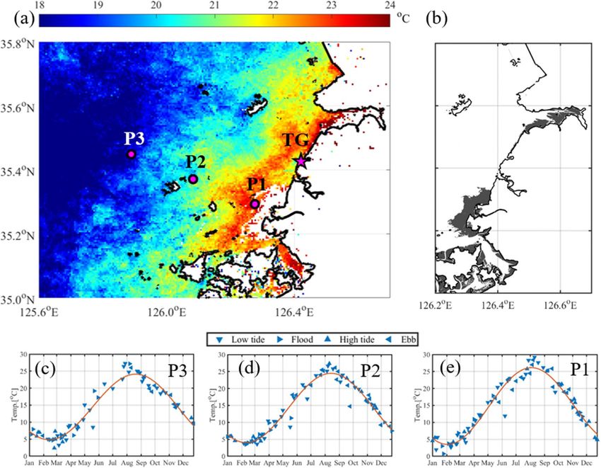
www.nature.com/scientificreports/
Figure 1. True color composite (RGB) image from Landsat 8 on February 21, 2019 in the study area. Blue boxes
represent the boundary of Landsat 8 scene and the red box represents the study area. Red circles (K1 and K2)
and red squares (J1 and J2) represent the location of buoy operated by Korea Hydrographic and Oceanographic
Agency (KHOA) and JNSI, respectively. Black line and gray area represent the coastal line and tidal flat,
respectively. Figures were generated by S.-T. Lee using MATLAB R2020a (http://www.mathworks.com).
obtains high-resolution images (30 m resolution of visible and near infrared band, and 60 m or 100 m resolution
of thermal infrared band). The Landsat data have been used to extract the waterline of Gomso Bay located on
the west coast of K orea16 and coast of China20.
Landsat satellite data enable us to distinguish among sea, tidal flat, landmass, and coastal lines and to estimate
surface temperatures of sea and land from brightness temperature. This can allow a high-resolution SST distri-
bution in coastal seas. SST variability and SST gradient were quantified by using Landsat TM band 6 thermal
infrared images on the central coast of M aine2. Climate observations of SST from Landsat TM and ETM + thermal
infrared data showed that isolated and shallow waters had larger temperature variations than well-connected
embayments or coastal oceans5.
Although many studies based on satellite-observed data have reported the spatial variations of SST in the
coastal sea, the variability of the water temperature near a macro tidal flat is ill-understood. In this study, the
characteristics of the SST distribution on the west coast of Korea were analyzed based on Landsat 8 data (Fig. 1).
The west coast of Korea is one of the regions where the tidal flat is widely distributed owing to the area’s large
tidal range and shallow water depth. Data from Landsat 8 from 2013 were analyzed to calculate SST using the
split-window algorithm for bands 10 and 11.
Results and discussion
Large seasonal variability of SST near tidal flat. SST from Landsat 8 was analyzed to examine the sea-
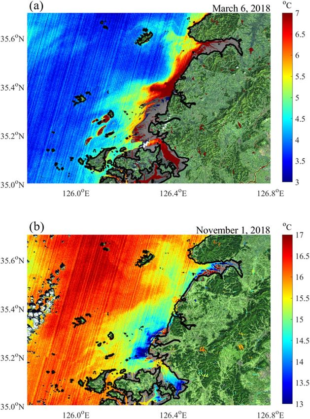
sonal variation in the SST near the macro tidal flat. Figure 2 shows the horizontal distribution of SST on March
6, 2018, and November 1, 2018, which represent the heating and cooling seasons, respectively. Most of the tidal
flats were exposed in each scene. SSTs near the Baeksu tidal flat, Hampyeong Bay, and Gomso Bay were warmer
than those in the open sea in March but colder in November.
The retrieved SST from Landsat 8 was interpolated at each grid with a resolution of 0.005°. All available data
at each grid were arranged on the Julian day to investigate seasonal variation, regardless of the observed year.
Three continuous years of repeated data were fitted into a 12th-order polynomial. The fitted data in the central
year were selected for analysis5. The tidal flat and land were excluded from the calculation. The seasonal SST
range was calculated from the difference between the maximum and minimum temperatures from the fitted
curve for each grid. The seasonal range of SST from Landsat 8 was calculated (Fig. 3). A large range of SST was
observed near the tidal flat in the seasonal variation (Fig. 3a). The wider the tidal flat distribution, the larger the
seasonal range (Fig. 3b). The seasonal range of SST near the tidal flat was larger by 5 °C than that in the open
sea. The minimum range in the open ocean is about 18 °C. However, the maximum range of coastal SST exceeds
23 °C, which is significantly greater than the 14 °C in the bay of Southern New E ngland5.
Three grid points: P1 (126.28° E, 35.29° N), P2 (126.08° E, 35.37° N), and P3 (125.89° E, 35.45° N), were
selected for the spatial comparison of the annual variations in SST (Fig. 3c,d). The temperature ranges were
22.6 °C, 20.46 °C, and 19.27 °C at grid points P1, P2, and P3, respectively. The maximum temperature at P1
was the highest among the three grid points, but the minimum temperature was the lowest. The maximum and
minimum temperatures at P1 appeared 17 days earlier compared to P3. The closer to the tidal flat, the higher the
maximum SST and the lower the minimum SST, resulting in an increase in seasonal range. The maximum and
minimum temperatures near the tidal flat appeared earlier than they do in the open sea.
Cause of large variability in SST near the tidal flat. A large horizontal SST gradient attributed to spa-
tially uneven heating or cooling in the coastal seas has been reported in previous studies2,5,21–23. The large vari-
ability in the SST near the macro tidal flat might have affected the horizontal SST gradient in our study area. Two
Scientific Reports | (2022) 12:248 | https://doi.org/10.1038/s41598-021-04465-4 2
Vol:.(1234567890)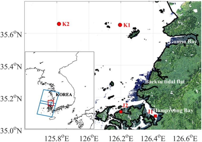
www.nature.com/scientificreports/
Figure 2. Sea surface temperature derived from Landsat 8 on (a) March 6, 2018 and (b) November 1, 2018.
The pixels corresponding to the tidal flat are marked in gray. The pixels corresponding to the land are marked
as RGB of the Landsat 8. The thick solid line represents the coastline. The clouds are presented in white. Figures
were generated by S.-T. Lee using MATLAB R2020a (http://www.mathworks.com).
lines were selected to estimate the effect of the tidal flat on the SST variability: line L1 near the Baeksu tidal flat
and line L2 far from the tidal flat (Fig. 4a). The horizontal SST gradient along each line was calculated for each
month (Fig. 4b). The red and blue lines represent the horizontal SST gradients along lines L1 and L2, respectively.
A negative value means that SST decreases onshore, and a positive value that SST increases onshore. The SST in
both lines commonly decreased onshore in fall and winter (January, February, October, November, and Decem-
ber), but increased in spring and summer. However, the seasonal variation of the SST gradient along line L1 was
remarkably larger than that along line L2. In winter, the coastal water temperature in line L1 was slightly lower
than that in line L2, but higher in summer. The minimum and maximum gradients along line L1 were approxi-
mately − 0.76 °C/10 km in December and approximately 1.31 °C/10 km in June, respectively. These gradients are
significantly larger than the minimum (− 0.44 °C/10 km) in January and the maximum (0.5 °C/10 km) in July on
the coast of Maine2. The minimum and maximum gradients along line L2 were approximately − 0.56 °C/10 km
in December, and approximately 0.99 °C/10 km in June, respectively.
Certain studies on the heat exchange between tidal flats and seawater have been conducted in areas where tidal
istributed6–8,14. The seasonal difference between the water temperature gradients of lines L1 and
flats are widely d
L2 might be due to the heat exchange between the tidal flat and sea water. The water temperature was vertically
homogeneous in the study area owing to active vertical mixing by strong tidal currents. The SST depends on the
water depth in a well-mixed shallow sea where the advection effect is not s ignificant5,22,24.
The horizontal temperature gradient in line L1 was remarkably larger despite a similar gradient of water depth.
The calculated gradient of water depth along each line calculated using gridded bathymetric data of 30 s was
5.49 m/10 km for line L1, and 5.61 m/10 km for line L 225. The larger gradient along line L1 despite the similar
water depth gradient implies that the tidal flat near line L1 acts as a sink or source of heat.
The additional heat at the onshore end point (red star in Fig. 4a) of line L1 was estimated from the horizontal
SST gradient difference between the two lines. The additional heat flux, which causes a relatively large horizon-
tal gradient of water temperature in line L1, was estimated based on the relative water temperature difference
between two onshore end points in both lines. The estimated additional heat flux at the end point of line L1 for
each month is shown in Fig. 5b. The black line represents the required monthly heat flux, and the gray vertical
bars represent one standard deviation. In June, the standard deviation was low owing to the lack of usable scenes
because of cloud contamination. The estimated heat flux shows a large seasonal variation (− 4.85 W/m2 to 6.72 W/
m2). This implies that sea water gains heat from the tidal flat in spring and summer and loses heat to the tidal
Scientific Reports | (2022) 12:248 | https://doi.org/10.1038/s41598-021-04465-4 3
Vol.:(0123456789)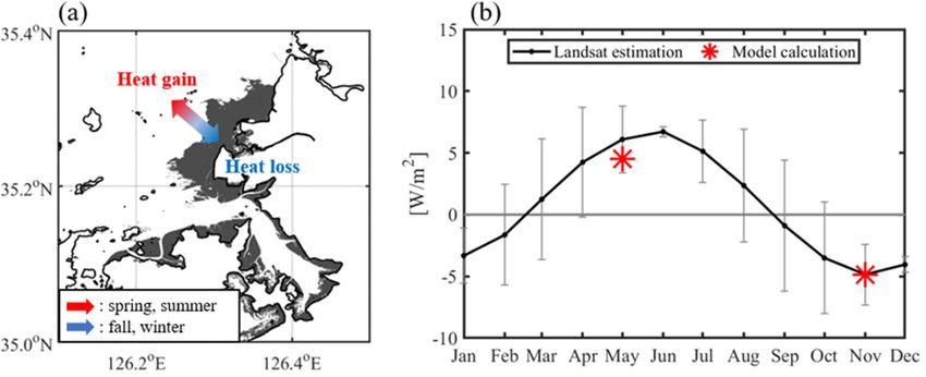
www.nature.com/scientificreports/
Figure 3. Horizontal seasonal range of the sea surface temperature near the tidal flat and a time series of sea
surface temperature at different points. (a) Seasonal range of the sea surface temperature calculated from the
difference between the maximum and minimum temperatures of the fitted seasonal variation at each pixel. The
magenta star represents the Yeonggwang tidal station. (b) Distribution of the tidal flat in the study area. Tidal
flats are marked in gray. Time series of sea surface temperature at grid points (c) P3, (d) P2, and (e) P1. Blue
triangles represent the tidal period when the SST was retrieved. Downward, rightward, upward, and leftward
triangles represent the low tide, flood, high tide and Ebb period, respectively. The red line represents a fitted
SST curve with a 12th order polynomial equation. Figures were generated by S.-T. Lee using MATLAB R2020a
(http://www.mathworks.com).
Figure 4. (a) Lines selected for the calculation of horizontal temperature gradient. Tidal flats are marked
as gray. (b) Horizontal temperature gradient per 10 km derived from Landsat 8 along line L1 (red) near the
tidal flat and along line L2 (blue) in far proximity from the tidal flat. Figures were generated by S.-T. Lee using
MATLAB R2020a (http://www.mathworks.com).
Scientific Reports | (2022) 12:248 | https://doi.org/10.1038/s41598-021-04465-4 4
Vol:.(1234567890)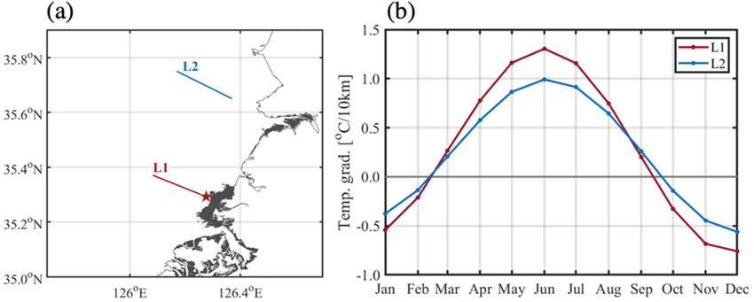
www.nature.com/scientificreports/
Figure 5. (a) Schematic diagram of heat exchange between the tidal flat and the seawater. Red arrow represents
that sea water gain heat from tidal flat in spring and summer. Blue arrow represents that sea water loss heat to
tidal flat in fall and winter. (b) Monthly heat exchange between the tidal flat and seawater at the red point of
L1 (Fig. 4) estimated from Landsat 8 data. The vertical bar represents one standard deviation in each month.
The red star is the heat exchange between the seawater and tidal flat calculated in previous s tudy8. Figures were
generated by S.-T. Lee using MATLAB R2020a (http://www.mathworks.com).
flat in fall and winter (Fig. 5a). A previous study8 calculated the heat exchange between Baeksu tidal flat and
seawater using the unstructured grid, finite-volume coastal ocean model (FVCOM) with a code for calculating
the sediment temperature according to the heat exchange between seawater and the seabed. Here, the tidal flat
supplied maximum heat to the seawater in May, and the gained maximum heat from the seawater in November.
The estimated heat fluxes are comparable with the calculated heat exchange between the tidal flat and seawater
based on model calculation in May and November (red stars in Fig. 5b). The calculated heat exchange in our
study area was 4.50 W m−2 in May and − 4.86 W m−2 in November8. The results reported by a previous model
study8 were within one standard deviation of our estimation.
Conclusions
Landsat 8 data enabled us to figure out the large variability of SST near the macro tidal flat on the west coast
of Korea, which has not been accessed for in-situ observation. SSTs derived from three different methods were
evaluated using in-situ data observed using buoys.
The seasonal range of SST near the tidal flat was approximately 23 °C, whereas it is approximately 18 °C in
the open seas. The maximum and minimum water temperatures near the tidal flat appeared approximately one
month earlier than they did in the open sea. The minimum and maximum gradients near the tidal flat were
approximately − 0.76 °C/10 km in December and approximately 1.31 °C/10 km in June. However, those far
from the tidal flat were approximately − 0.56 °C/10 km in December and approximately 0.99 °C/10 km in June,
respectively. Seasonal changes in the horizontal SST gradient were high because of the heat exchange between
the tidal flat and sea water. The estimated heat exchange between the tidal flat and seawater based on Landsat 8
data was comparable with that of a previous study based on model calculation. The estimated heat flux from the
tidal flat to the seawater exhibited large seasonal variation, with a minimum of − 4.85 W/m2 in December and a
maximum of 6.72 W/m2 in June.
Our study suggests that the extensive utilization of Landsat 8 in research in macro tidal flat areas is expected.
However, additional efforts based on in-situ observations and numerical model experiments are required to
support our findings.
Methods
Landsat 8 data processing. Data contaminated by clouds should be removed to obtain an accurate SST.
Landsat 8 provides the band quality for each pixel. Pixel values of 2720, 2724, 2728, and 2732, regarded as cloud-
free, were removed. However, cloud detection based on pixel quality is limited in the removal of sea fog and low
clouds. RGB data were additionally examined to exclude pixels contaminated by clouds. After removing cloud
pixels, the others were classified into land, tidal flat, and sea water. The brightness temperature of Landsat 8 was
also compared with the buoy observation data to remove data contaminated by clouds.
Classifying Landsat data into seawater, tidal flats, and land for this study was crucial. The near infrared band is
more beneficial to distinguish between water and other regions, because the reflectivity of water decreases while
that of non-water increases as the visible band approaches the near infrared band. So, the regions with water and
non-water could be easily distinguished through histograms of the near infrared band near a coastal area which
shows a clear bimodal distribution. This is consistent with the results of a previous study investigating another
orea22. Sometimes, in the case of a non-water region, the bimodal structure lacks clarity due
tidal flat in South K
to a lack of vegetation that causes the upland to also be included, rather than only the exposed tidal flat. To solve
this problem, the upland area was removed by NDVI in advance. The Landsat normalized difference vegetation
Scientific Reports | (2022) 12:248 | https://doi.org/10.1038/s41598-021-04465-4 5
Vol.:(0123456789)www.nature.com/scientificreports/
index (NDVI), useful for understanding vegetation density and changes in plant health, was used to define land
(https://www.usgs.gov/). The NDVI is determined as follows:
Band 5 − Band 4
NDVI = . (1)
Band 5 + Band 4
The digital number of the near infrared band of each Landsat 8 scene shows three peaks in a histogram. The
three peaks correspond to the sea, tidal flat, and landmass in digital numbers. Pixels with digital numbers cor-
responding to the sea, tidal flat, and landmass were classified at each scene according to a previous method26. A
previous study26 using the near infrared band reported that its accuracy was within about 69 m, which is sufficient
to demarcate the tidal flat of this study.
Landsat 8, equipped with an Operational Land Imager (OLI) and a Thermal Infrared Sensor (TIRS), was
launched on February 11, 2013. The TIRS of Landsat 8 comprises two thermal infrared channels and can correct
atmospheric effects using a split-window a lgorithm27. Band 10 covers the wavelength range of 10.6–11.2 μm and
band 11, 11.5–12.5 μm28. The split-window algorithm was used to calculate the land surface temperature (LST)
or water surface temperature (WST) using the warm temperatures of the two bands29–34. In this study, SST using
three different algorithms proposed by Rongali et al.33, Vanhellemenot31, and Jang and Park32, were compared
with the observation data to determine the optimal coastal region temperature.
All Landsat 8 OLI/TIRS data were obtained from NASA and the United States Geological Survey (USGS)
(https://e arthe xplor er.u
sgs.g ov/). Two scenes (scene numbers 116,035 and 116,036), including the study area and
(Fig. 1), from January 2014 to May 2021 were analyzed. The scenes were captured at approximately 11 am (LT)
every 16 days. The brightness temperatures of bands 10 and 11 provided by the USGS were used in this study.
The algorithm proposed by Rongali et al.33 was adapted to obtain the SST as follows:
SST R = BT 10 +C 1 (BT 10 − BT 11 )+C 2 (BT 10 − BT 11 )2 +C 0 +(C 3 + C 4 W)(1 − m)+(C 5 + C 6 W)�m.
(2)
BT 10 and BT 11 are the brightness temperatures (°C) of bands 10 and 11, respectively. C 0 to C 6 is the split-
window (SW) coefficient value33,35,36. m is the mean of the water surface emissivity (WSE) of the TIRS bands
((WSE10 + WSE 11 )/2), W is the atmospheric water vapor content, and m is the difference in the WSE
( WSE10 − WSE 11 ). Regarding water vapor content, the split-window covariance-variance ratio method and
16 × 16 adjacent pixels were used for calculation at every scene and p ixel37. The WSEs of bands 10 and 11 are
0.9926 and 0.9877, r espectively31.
SST proposed by Vanhellemenot31 was calculated as follows:
1−m �m BT10 + BT11
SSTV =b0 + b1 + b2 + b3 2
m m 2
(3)
1−m �m BT10 − BT11
+ b4 + b5 + b6 2 + b7 (BT10 − BT11 )2
m m 2
The bn(n = 0 to 7) coefficients were derived from simulations by Du et al.34 based on the ranges of column
water vapor (g/cm2). In this study, we used coefficient bn ranging from 0 to 6.3 g/cm2.
A formula for obtaining multi-channel SST (MCSST) from Landsat 8 data through a matchup with buoy data
in the coastal sea of the Korean peninsula was proposed by Jang and P ark32 from April 2013 to August 2017.
Like the previous two algorithms, the MCSST algorithm can compute SSTs in two independent ways. MCSST1,
which uses only the brightness temperatures of bands 10 and 11 among MCSSTs, was selected for this study.
Following is the MCSST1 formula:
SSTJ = a1 BT11 + a2 (BT10 − BT11 ) + a3 . (4)
a1, a2, and a3 are 0.9767, 1.8362, and 0.0699, respectively.
Comparison of SSTs. SSTs from moored buoys were used to evaluate three different water surface tem-
perature algorithms (Fig. 1). Buoys J1 and J2 have been operated by the Jeonnam Sea Information Center (JSIC)
since July 29, 2019. The locations of J1 and J2 are 126.41449° E, 35.0830° N, and 126.1977716° E, 35.111225° N,
respectively (https://jnsi.jeonnam.go.kr/). Data are accessible to parties authorized by the JSIC. They provided
hourly SST data observed by buoys. Buoy SST data obtained within the period that were closest to those of
Landsat 8 were selected for comparison.
Buoy K1 is operated by the Korea Hydrographic and Oceanographic Agency (KHOA). The data can be down-
loaded from KHOA’s real-time ocean observation information system (http://w ww.k hoa.g o.k r). Buoy K1, located
at 126.194255° E, 35.652458° N, provides a 30-min interval SST from January 1, 2015 to December 31, 2019.
Buoy K2, located at 125.8139° E, 35.6586° N, is operated by the Korea Meteorological Administration (KMA).
Data were downloaded from the KMA Weather Data Service (https://d ata.k ma.g o.k r/). Buoy K2 provided hourly
SST data from December 22, 2015. In this study, buoy data from December 22, 2015 to March 27, 2021 were
compared with the SST data obtained from Landsat 8. SST values exceeding twice the standard deviation in each
month for buoys K1 and K2 were removed.
The SST derived from Landsat 8 using three algorithms were compared with in-situ SST data at buoys. The
root mean square error (RMSE) for the three SST and in-situ SST data were calculated for each buoy (Fig. 1).
The three retrieval temperatures were in good agreement with the in-situ temperature. The RMSE was seasonally
different (Supplementary Fig. S1). The maximum peak in June appeared in all the methods. The high RMSE in
Scientific Reports | (2022) 12:248 | https://doi.org/10.1038/s41598-021-04465-4 6
Vol:.(1234567890)www.nature.com/scientificreports/
June might be affected by high relative humidity during the rainy season. The RMSE of SSTR considering the
humidity effect was lowest in July, whereas that of S STJ was lowest in March, April, October, November, and
December. The overall performance of SSTJ was optimal, except for the high humidity period, because SSTJ
uses optimized coefficients through fitting between brightness temperatures and in-situ temperatures on the
Korean coast, which includes our study area, whereas S STR and SSTV adopt common coefficients depending on
water vapor regardless of region. This suggests that S STJ represents the open sea temperature and coastal water
temperature. SSTJ corresponds to the in-situ SST at all buoys. R 2 was 0.99 at buoys J1 and J2, and 0.98 at buoys
K1 and K2. This result suggests that S STJ represents open sea temperature and coastal water temperature.
Heat exchange between tidal flat and sea water. We can assume that the ratio between the horizon-
tal SST gradients and the depth change is the same along both lines, where the effects of the river and current
are not significant. The relationship between the horizontal water temperature gradient and the horizontal depth
gradient can be expressed as follows:
Wgrad1 Wgrad2
= , (5)
dgrad1 dgrad2
where, wgrad1 and wgrad2 are the horizontal water temperature gradients (°C/m) along lines L1 and L2, respectively,
and dgrad1 and dgrad2 are the horizontal depth gradients(m/m) along lines L1 and L2, respectively.
The additional heat flux per unit area ( m2) for line L1 relative to line L2 was calculated using Eq. (6).
q = T × C × m, (6)
where, q (J/m2) is the required heat sink or source, m (g) is the mass of seawater, and T (°C) is the relative
water temperature difference between the two onshore endpoints in both lines. The mass value per unit area at
a depth of 4.9 m at the red point of L1 in Fig. 4a was used. C is the specific heat of water and is 4.184 J/g °C.
T was calculated as follows:
wgrad2
T = wgrad1 − × dgrad1 × lengthL1 . (7)
dgrad2
lengthL1 is the length of line L1. The temperature dependence of the water depth along both lines was assumed
to be the same as that in previous s tudies5,22,24.
Data availability
The data availability is outlined in “Methods” section. Correspondence and requests for materials should be
addressed to S.-T.L and Y.-K.C.
Received: 29 September 2021; Accepted: 15 December 2021
References
1. Palmer, T. N. & Zhaobo, S. A modelling and observational study of the relationship between sea surface temperature in the North-
West Atlantic and the atmospheric general circulation. Q. J. R. Meteorol. Soc. 111, 947–975 (1985).
2. Thomas, A., Byrne, D. & Weatherbee, R. Coastal sea surface temperature variability from Landsat infrared data. Remote Sens.
Environ. 81, 262–272 (2002).
3. Josey, S. A., Somot, S. & Tsimplis, M. Impacts of atmospheric modes of variability on Mediterranean Sea surface heat exchange. J.
Geophys. Res. Ocean 116, 1–15 (2011).
4. Loschnigg, J. & Webster, P. J. A coupled ocean–atmosphere system of SST modulation for the Indian Ocean. J. Clim. https://doi.
org/10.1175/1520-0442(2000)013%3c3342:ACOASO%3e2.0.CO;2 (2000).
5. Fisher, J. I. & Mustard, J. F. High spatial resolution sea surface climatology from Landsat thermal infrared data. Remote Sens.
Environ. 90, 293–307 (2004).
6. Vugts, H. F. & Zimmerman, J. T. F. The heat balance of a tidal flat area. Neth. J. Sea Res. 19, 1–14 (1985).
7. Kim, T. W., Cho, Y. K., You, K. W. & Jung, K. T. Effect of tidal flat on seawater temperature variation in the southwest coast of
Korea. J. Geophys. Res. Ocean 115, 1–15 (2010).
8. Kim, T. W. & Cho, Y. K. Calculation of heat flux in a macrotidal flat using FVCOM. J. Geophys. Res. Ocean. https://d oi.o
rg/1 0.1 029/
2010JC006568 (2011).
9. Dyer, K. R., Christie, M. C. & Wright, E. W. The classification of intertidal mudflats. Cont. Shelf Res. 20, 1039–1060 (2000).
10. Beukema, J. J. Annual variation in reproductive success and biomass of the major macrozoobenthic species living in a tidal flat
area of the Wadden Sea. Neth. J. Sea Res. 16, 37–45 (1982).
11. Nakata, H., Sakai, Y., Miyawaki, T. & Takemura, A. Bioaccumulation and toxic potencies of polychlorinated biphenyls and polycyclic
aromatic hydrocarbons in tidal flat and coastal ecosystems of the Ariake Sea, Japan. Environ. Sci. Technol. 37, 3513–3521 (2003).
12. McQuaid, C. & Branch, G. Influence of sea temperature, substratum and wave exposure on rocky intertidal communities: An
analysis of faunal and floral biomass. Mar. Ecol. Prog. Ser. 19, 145–151 (1984).
13. Ottersen, G. & Sundby, S. Effects of temperature, wind and spawning stock biomass on recruitment of Arcto-Norwegian cod. Fish.
Oceanogr. 4, 278–292 (1995).
14. Yanagi, T., Sugimatsu, K., Shibaki, H., Shin, H. R. & Kim, H. S. Effect of tidal flat on the thermal effluent dispersion from a power
plant. J. Geophys. Res. C Ocean 110, 1–15 (2005).
15. Gidhagen, L. Coastal upwelling in the Baltic Sea-Satellite and in situ measurements of sea-surface temperatures indicating coastal
upwelling. Estuar. Coast. Shelf Sci. 24, 449–462 (1987).
16. Plattner, S., Mason, D. M., Leshkevich, G. A., Schwab, D. J. & Rutherford, E. S. Dynamics of wind-induced coastal upwelling and
interbasin exchange in Lake Geneva during winter. J. Great Lakes Res. 32, 63–76 (2021).
17. Benazzouz, A. et al. An improved coastal upwelling index from sea surface temperature using satellite-based approach—The case
of the Canary Current upwelling system. Cont. Shelf Res. 81, 38–54 (2014).
Scientific Reports | (2022) 12:248 | https://doi.org/10.1038/s41598-021-04465-4 7
Vol.:(0123456789)www.nature.com/scientificreports/
18. Ginzburg, A. I., Kostianoy, A. G. & Sheremet, N. A. Seasonal and interannual variability of the Black Sea surface temperature as
revealed from satellite data (1982–2000). J. Mar. Syst. 52, 33–50 (2004).
19. Loveland, T. R. & Irons, J. R. Landsat 8: The plans, the reality, and the legacy. Remote Sens. Environ. 185, 1–6 (2016).
20. Wang, X. et al. Tracking annual changes of coastal tidal flats in China during 1986–2016 through analyses of Landsat images with
Google Earth Engine. Remote Sens. Environ. 238, 110987 (2020).
21. Fox, M. F., Kester, D. R., Andrews, J. E., Magnuson, A. & Zoski, C. G. Seasonal warming of Narragansett Bay and Rhode Island
Sound in 1997: Advanced very high resolution radiometer sea surface temperature and in situ measurements. Journal of Geophysical
Research. 105, 71–82 (2000).
22. Mustard, J. F., Carney, M. A. & Sen, A. The use of satellite data to quantify thermal effluent impacts. Estuar. Coast. Shelf Sci. 49,
509–524 (1999).
23. Uncles, R. J. & Stephens, J. A. The annual cycle of temperature in a temperate estuary and associated heat fluxes to the coastal zone.
J. Sea Res. 46, 143–159 (2001).
24. Prandle, D. & Lane, A. The annual temperature cycle in shelf seas. Cont. Shelf Res. 15, 681–704 (1995).
25. Seo, S.-N. Digital 30sec gridded bathymetric data of Korea marginal seas—KorBathy30s. J. Korean Soc. Coast. Ocean Eng. 20,
110–120 (2008).
26. Ryu, J. H., Won, J. S. & Min, K. D. Waterline extraction from Landsat TM data in a tidal flat a case study in Gomso Bay, Korea.
Remote Sens. Environ. 83, 442–456 (2002).
27. Coll, C. & Caselles, V. A split-window algorithm for land surface temperature from advanced very high resolution radiometer
data: Validation and algorithm comparison. J. Geophys. Res. Atmos. 102, 16697–16713 (1997).
28. Barsi, J. A., Lee, K., Kvaran, G., Markham, B. L. & Pedelty, J. A. The spectral response of the Landsat-8 operational land imager.
Remote Sens. 6, 10232–10251 (2014).
29. Rozenstein, O., Qin, Z., Derimian, Y. & Karnieli, A. Derivation of land surface temperature for landsat-8 TIRS using a split window
algorithm. Sensors (Switzerland) 14, 5768–5780 (2014).
30. Yu, X., Guo, X. & Wu, Z. Land surface temperature retrieval from landsat 8 TIRS-comparison between radiative transfer equation-
based method, split window algorithm and single channel method. Remote Sens. 6, 9829–9852 (2014).
31. Vanhellemont, Q. Automated water surface temperature retrieval from Landsat 8/TIRS. Remote Sens. Environ. 237, 111518 (2020).
32. Jang, J. C. & Park, K. A. High-resolution sea surface temperature retrieval from Landsat 8 OLI/TIRS data at coastal regions. Remote
Sens. 11, 2687 (2019).
33. Rongali, G., Keshari, A. K., Gosain, A. K. & Khosa, R. Split-window algorithm for retrieval of land surface temperature using
Landsat 8 thermal infrared data. J. Geovis. Spat. Anal. https://doi.org/10.1007/s41651-018-0021-y (2018).
34. Du, C., Ren, H., Qin, Q., Meng, J. & Zhao, S. A practical split-window algorithm for estimating land surface temperature from
Landsat 8 data. Remote Sens. 7, 647–665 (2015).
35. Sobrino, J. A., Jiménez-Muñoz, J. C. & Paolini, L. Land surface temperature retrieval from LANDSAT TM 5. Remote Sens. Environ.
90, 434–440 (2004).
36. Zhao, S., Qin, Q., Yang, Y., Xiong, Y. & Qiu, G. Comparison of two split-window methods for retrieving land surface temperature
from MODIS data. J. Earth Syst. Sci. 118, 345–353 (2009).
37. Ren, H. et al. Atmospheric water vapor retrieval from Landsat 8 and its validation. Int. Geosci. Remote Sens. Symp. https://doi.org/
10.1109/IGARSS.2014.6947119 (2014).
Acknowledgements
This research study was carried out as a part of the project titled “Deep Water Circulation and Material Cycling
in the East Sea (0425-20170025)” funded by the Ministry of Oceans and Fisheries, Republic of Korea.
Author contributions
S.-T.L., Y.-K.C. and D.-J.K. designed the study. S.-T.L. performed the data analysis. S.-T.L. wrote the main
manuscript, including the figures. S.-T.L., Y.-K.C. and D.-J.K. reviewed the manuscript and Y.-K.C. revised the
manuscript.
Competing interests
The authors declare no competing interests.
Additional information
Supplementary Information The online version contains supplementary material available at https://doi.org/
10.1038/s41598-021-04465-4.
Correspondence and requests for materials should be addressed to Y.-K.C.
Reprints and permissions information is available at www.nature.com/reprints.
Publisher’s note Springer Nature remains neutral with regard to jurisdictional claims in published maps and
institutional affiliations.
Open Access This article is licensed under a Creative Commons Attribution 4.0 International
License, which permits use, sharing, adaptation, distribution and reproduction in any medium or
format, as long as you give appropriate credit to the original author(s) and the source, provide a link to the
Creative Commons licence, and indicate if changes were made. The images or other third party material in this
article are included in the article’s Creative Commons licence, unless indicated otherwise in a credit line to the
material. If material is not included in the article’s Creative Commons licence and your intended use is not
permitted by statutory regulation or exceeds the permitted use, you will need to obtain permission directly from
the copyright holder. To view a copy of this licence, visit http://creativecommons.org/licenses/by/4.0/.
© The Author(s) 2022
Scientific Reports | (2022) 12:248 | https://doi.org/10.1038/s41598-021-04465-4 8
Vol:.(1234567890)You can also read