Improving cold-region streamflow estimation by winter precipitation adjustment using passive microwave snow remote sensing datasets - IOPscience
←
→
Page content transcription
If your browser does not render page correctly, please read the page content below

LETTER • OPEN ACCESS

Improving cold-region streamflow estimation by winter precipitation
adjustment using passive microwave snow remote sensing datasets
To cite this article: D Kang et al 2021 Environ. Res. Lett. 16 044055

View the article online for updates and enhancements.

                                This content was downloaded from IP address 46.4.80.155 on 22/08/2021 at 13:01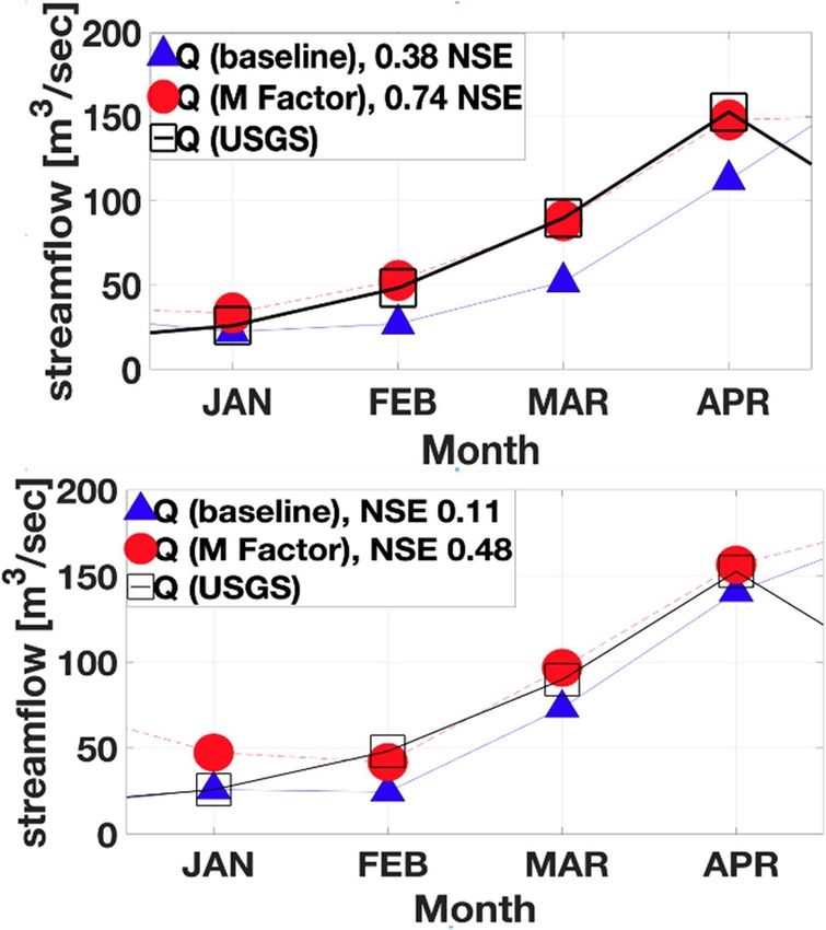
Environ. Res. Lett. 16 (2021) 044055 https://doi.org/10.1088/1748-9326/abe784
LETTER
Improving cold-region streamflow estimation by winter
OPEN ACCESS
precipitation adjustment using passive microwave snow remote
RECEIVED
25 July 2020 sensing datasets
REVISED
16 February 2021 D Kang1,2,∗, K Lee1,2 and E J Kim2
ACCEPTED FOR PUBLICATION 1
18 February 2021 Earth System Interdisciplinary Center, University of Maryland, College Park, MD 20740, United States of America
2
NASA Goddard Space Flight Center, Greenbelt, MD 20771, United States of America
PUBLISHED ∗
Author to whom any correspondence should be addressed.
8 April 2021
E-mail: dk.kang@nasa.gov
Original content from Keywords: winter precipitation adjustment, snow water equivalent, AMSR-E (advanced microwave scanning radiometer-E),
this work may be used
under the terms of the hydrologic model, streamflow prediction
Creative Commons Supplementary material for this article is available online
Attribution 4.0 licence.
Any further distribution
of this work must
maintain attribution to Abstract
the author(s) and the title
of the work, journal Winter precipitation estimations and spatially sparse snow observations are key challenges when
citation and DOI.
predicting snowmelt-driven floods. An improvement in streamflow prediction is achieved in a
snowmelt-dominant basin, i.e. the Red River Basin (RRB), by adjusting the amounts of snowfall
through satellite-borne passive microwave observations of snow water equivalent (SWE). A
snowfall forcing dataset is scaled to minimize the difference between simulated and observed SWE
over the RRB. Advanced microwave scanning radiometer-E (AMSR-E) SWE products serve as the
observed SWE to obtain the solution to the linear equation between the AMSR-E and the baseline
(no snowfall-forcing adjustment) SWE to yield a multiplication factor (M factor ). In the headwaters
of the RRB in the United States, a Nash–Sutcliffe efficiency (NSE) of 0.74 is obtained against
observed streamflow, with M factor -adjusted streamflow during the snowmelt seasons (January to
April). The baseline streamflow simulation without M factor exhibits an NSE of 0.38 owing to an
underestimated SWE.
1. Introduction for hydrologic modeling applications [7, 8]. Adams
and Lettenmaier [9] adjusted the bias of global winter
Cold region hydrological processes have garnered precipitation, but the source of adjustments was from
increasing attention because of climate change and its point-based meteorological observations. Andreadis
hydrological effects on communities where snow and and Lettenmaier [10] assimilated the SWE using a
ice are essential to the water supply [1]. Estimation remote sensing dataset, including passive microwave
of the amount of snowmelt runoff remains challen- observations; however, streamflow was not simu-
ging despite long-term concerns regarding the applic- lated as a criterion for performance improvement.
ations of water resources, which are associated with Shi et al [11] evaluated cold region hydrological
snow hydrology [2–5]. Cold region hydrological pro- processes in the Northern Hemisphere using bias-
cesses have different characteristics that are affected corrected winter precipitation to demonstrate recent
not only by rainfall, but also by the release of snow- changes induced by climate change in the cryo-
melt, which depends on the distribution of the snow sphere to evaluate the degree to which streamflow
water equivalent (SWE) and the timing of melts in prediction is improved using the adjusted winter
the basin. In climatology, in addition to the finer-scale precipitation in subarctic watersheds. Despite the
hydrological cycle, snow is regarded as a sensitive ele- importance of snow, exact mass measurements and
ment for the evaluation of climate variations at both spatially varying snowfall monitoring are unreli-
local and global scales [6]. able when using traditional or sophisticated obser-
Winter precipitation corrections for mountain- vational technologies, including in-situ precipitation
ous areas have been attempted by many researchers gauges, and ground-based precipitation radars [12].
© 2021 The Author(s). Published by IOP Publishing Ltd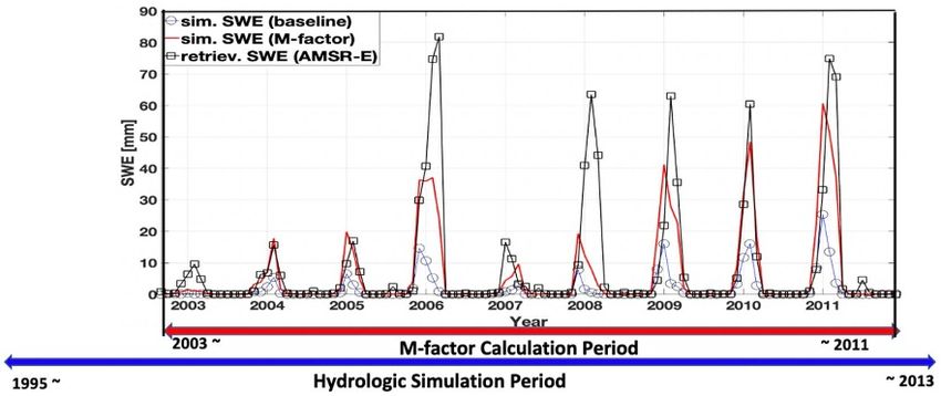
Environ. Res. Lett. 16 (2021) 044055                                                                     D Kang et al

Furthermore, measurement errors associated with              microwave radiometer from the National Aeronautics
a precipitation gauge range from 20% to 50% as               and Space Administration Aqua satellite for years
compared with the actual snowfall; this is typically         2002–2011. Satellite passive microwave products for
referred to as the ‘snow undercatch’ problem [13, 14].       the SWE are spatially distributed and temporally con-
Approximately half of all snowflakes at high wind            tinuous. Hence, they are appropriate for determin-
sites tend to be recorded using traditional precip-          ing the average amount of SWE over the domain
itation gauges owing to aerodynamic flows around             when the SWE is dry and does not exceed 150 mm.
the gauge [15]. This suggests that a multiplication          The two cases of simulated streamflow (baseline and
factor of approximately 2 is necessitated to accom-          M factor adjusted) were calibrated against the observed
modate the actual amount of snowfall to a land sur-          streamflow from stream gauge data available from
face at open and windy sites, such as the Northern           the U.S. Geological Survey (USGS). The hydrolo-
Great Plains. If a device for precipitation measure-         gic calibration/validation and streamflow analyses
ment is affected by snow undercatch, and a weather           were constrained to the snow-melting period from
forcing dataset is generated from these point precip-        January to April, not for an entire year. The aim of
itation observations, then a scaling factor to correct       this study was to determine the scaling factor for
the winter precipitation must be applied. Addition-          winter precipitation in a watershed in the Northern
ally, the factor must be constant across a watershed,        Great Plains for a specified period and then apply it
regardless of temporal variations. Owing to the het-         to the prediction of streamflow over a longer period
erogeneous distribution of terrestrial snow on com-          using a hydrologic model to demonstrate an improve-
plicated topographies, it is challenging to determine        ment in streamflow performance during the melt
the scaling factor in a watershed.                           season.
     Few modern snow hydrologic applications using
remote sensing have been implemented in the North-           2. Methods and materials
ern Great Plains [16, 17], as compared with the
numerous snow studies in the western United States.          This section provides details regarding the methods
In the Northern Great Plains, snow is the most det-          for scaling winter precipitation using the solution for
rimental source of flooding during spring snowmelt.          linear equations between the AMSR-E SWE and the
Snowmelt-driven floods directly affect the popula-           baseline hydrologic simulation. First, a description
tion along the rivers in the Northern Great Plains           of the application watershed is presented, followed
[18, 19] because of the flat topography and poorly           by the specifications of the hydrologic model and a
draining soil. These factors decrease the flow velo-         method for adjusting winter precipitation.
city of surface waters derived from the snowmelt
once it begins [20]. To demonstrate an improvement           2.1. RRB in the in the Northern Great Plains
in streamflow prediction by adjusting winter pre-            The RRB flows through two U.S. states and one Cana-
cipitation, a representative and well-observed water-        dian province, starting at the border between North
shed, the Red River Basin (RRB) in the Northern              Dakota and Minnesota, and ending in Manitoba,
Great Plains, was investigated. The headwaters of the        Canada. The catchment of this north-flowing river
RRB were selected to apply the proposed multiplic-           occupies 287 500 km2 , and springtime ice congestions
ation factor (M factor ) method to the underestimated        in the north result in considerable flooding because
winter precipitation to demonstrate the improvement          of the backwater effect of these frozen water bod-
in streamflow prediction.                                    ies [21]. In recent decades, the RRB has experienced
     Streamflow simulation driven by snowmelt                regular annual flooding incidents, causing national-
involves various nonlinear processes such as selec-          level concern [22]. The floods from January to April
tion of snow schemes, infiltration characteristics,          are primarily driven by fast snowmelt. Significant
and routing schemes after the land model is used.            community efforts have been expended with support
However, this study focused on the effect of snow-           from state and federal governments [23] to establish
melt on streamflow generation in a snowmelt-                 flood prediction and monitoring capabilities for res-
dominant watershed instead of other hydrological             idents throughout the main stem of the RRB. It is
processes. The hydrologic model was used twice,              critical to establish a monitoring system for spatially
i.e. (a) with a baseline hydrologic simulation with          distributed SWEs. Satellite passive microwave obser-
non-adjusted winter precipitation; and (b) with an           vations, with revisits twice per day, can be used to
adjusted winter precipitation hydrologic simulation          determine the daily status of the SWE throughout
scaled by M factor . The scaling factor of the winter pre-   the basin, thereby allowing observations of the peak
cipitation was derived from the solution for linear          amount of SWE.
equations between the advanced microwave scan-                   Figure 1 (left) depicts the location and extent
ning radiometer-E (AMSR-E) SWE and the baseline              of the RRB headwaters, to which this study was
SWE. We independently determined the amount                  applied, which has an area of 13 476 km2 . The out-
of SWE at each grid cell using the AMSR-E SWE.               let of the RRB headwaters is located in Fargo, ND
This was achieved by employing an AMSR-E passive             and was gauged using the USGS streamflow gauge

                                                2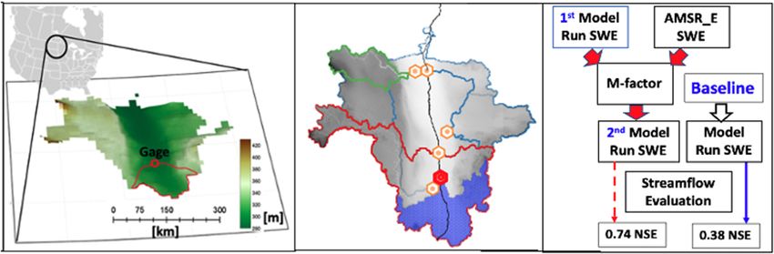
Environ. Res. Lett. 16 (2021) 044055                                                                                           D Kang et al

   Figure 1. Left: location of headwaters of RRB (center): headwaters and subwatersheds of RRB as well as locations of USGS
   streamflow gauges, and (right): two sets of hydrologic simulations with and without M factor for evaluating streamflow
   predictability. Arrows show sequential steps of M factor and the variable infiltration capacity (VIC) applications for streamflow
   evaluations.

ID 05054000. The enlarged view of the watershed                        stations using standard precipitation gauges. Wind
in figure 1 (center) provides a topographic repres-                    speeds were obtained from a reanalysis dataset from
entation of the RRB; the elevation difference over                     the National Centers for Environmental Prediction–
130 km of the river was 200 m, with an average                         National Center for Atmospheric Research [29].
slope of only 0.08◦ . The large area of the basin                      Point measurements were linearly interpolated from
and the rapid increase in air temperature during                       approximately 1.9◦ to 1/8◦ resolution, which is sim-
the spring season resulted in abrupt flooding in the                   ilar to the grid resolution used in the AMSR-E SWE
local municipalities, particularly along river banks                   retrieval.
in the Fargo metropolitan areas. An abrupt increase                         With the baseflow and runoff from the VIC
in the air temperature, coupled with the flat topo-                    considering snowmelt with three soil layers, classic
graphy, caused a free water body to form from the                      streamflow calibration was performed by minimizing
meltwater, and small melt ponds enlarged abruptly                      the cost function between the observed and simulated
owing to the poor drainage of the Northern Great                       streamflows at the outlets of a watershed [30, 31]. Cal-
Plains. The average maximum winter precipitation,                      ibrated soil parameters were applied to the validation
from December to March, is approximately 100 mm                        period to evaluate the accuracy of streamflow predic-
SWE, which is sufficient to create a large snow mass.                  tion. It is beyond the scope of this study to identify the
During wet winters, the peak SWE in the large basin                    optimal soil parameters to accurately represent the
can reach up to 200 mm, which is disastrous to                         overall peak of the streamflow associated with rain-
many communities when any abrupt melting occurs                        fall and snowmelt.
in the spring. For a general depiction of the cli-
matology of this region, figure S1 (available online                   2.3. Winter precipitation adjustment using
at stacks.iop.org/ERL/16/044055/mmedia) demon-                         AMSR-E SWE
strates the monthly snowfall, rainfall, and air temper-                The amount of winter precipitation in the model was
ature averaged from 1995 to 2013 in the headwaters                     adjusted with a factor to match with the amount
of the RRB.                                                            of SWE based on the U.S. AMSR-E SWE product
                                                                       (25 km), compared with the 12.5 km grid cell of
2.2. VIC-ROUT model setup                                              the VIC model. A M factor of winter precipitation was
In this study, a semi-distributed macroscale hydrolo-                  used to scale the winter precipitation in relation to
gical model known as the VIC model (version 4.0.6)                     the observed AMSR-E SWE. Despite the well-known
was used [24] in addition to a routing scheme, VIC-                    microwave saturation that occurs when the SWE
ROUT. The VIC model has been widely applied to                         exceeds 150 mm [32–34], the AMSR-E SWE offers
assess hydrological responses to weather and climate                   several advantages, including long temporal cover-
over numerous river basins globally [for example,                      age (2002–2011), near-daily observations, and global
25, 26]. The VIC model was used in this study                          spatial coverage [35]. The National Snow and Ice
for streamflow calibrations, with emphasis on the                      Data Center (NSIDC) archives the microwave bright-
snowmelt runoff in the headwaters of the RRB in                        ness temperature (Tb). The SWE products from the
the Northern Great Plains. Detailed descriptions                       AMSR-E Tb datasets were processed based on a spec-
of the snow scheme are included in pages 6–9 of                        tral difference between the 18.7 GHz Tb (least affected
the supplementary data. Precipitation and temperat-                    by snow) and the 36.5 GHz Tb (most affected by snow
ure observations were provided by weather stations,                    [36],). The period from 2002 to 2011 was used to
and the synergraphic mapping system algorithm                          encompass the global domain with a 25 km grid using
[27] was employed to generate gridded temperat-                        the equal area scalable earth grid (EASE-Grid) format
ures spatially interpolated from the point observa-                    from the NSIDC (later updated to EASE-Grid 2.0
tions [26, 28]. Specifically, the precipitation data were              [37]). A spatially averaged ratio was obtained using
obtained from NOAA cooperative observer (COOP)                         a solution for linear equations between the AMSR-E

                                                        3
Environ. Res. Lett. 16 (2021) 044055 D Kang et al
Figure 2. SWE intercomparison among VIC baseline, M factor -adjusted, and AMSR-E-retrieved SWEs. M factor calculation period
(2003–2011 hydrological years) and hydrologic simulation period (1995–2013) shown below x-axis.
based observed and the baseline simulated SWE in all data can be used to replace the AMSR-E SWE; how-
grid cells throughout the hydrologic years from 2003 ever, it is only applicable to well-observed watersheds
to 2011. The M factor was calculated using the following such as the RRB, where the number of observations is
equation: abundant. However, snow undercatch problems per-
sist in NOAA COOP stations.
[SWEVIC - baseline ]2003−2011 · Mfactor Figure 2 displays three basin-averaged SWE
= [SWEAMSR - E ]2003−2011 (1) estimates: the baseline VIC simulation, the M factor -
adjusted VIC simulation, and the AMSR-E SWE
observations. The spatially averaged ratio from
Mfactor = SWEAMSR - E · pinv (SWEVIC - baseline ) , (2) equation (1) during the M factor calculation period,
i.e. 2003–2011, was used as the scaling factor for
the winter precipitation at all 70 grid cells in the
where SWEAMSR-E is the AMSR-E-retrieved daily SWE
RRB headwater region and was applied to the
(mm), and SWEVIC-baseline is the VIC-simulated daily
longer hydrologic modeling period, i.e. 1995–2013,
SWE (mm) without M factor adjustment. M factor is
to demonstrate the validity of M factor outside the
determined by solving a system of linear equations
M factor calculation period. A M factor -adjusted hydro-
with the assumption that both time series are row vec-
logic simulation was performed to demonstrate the
tors of the same size from hydrological years 2003–
improved predictability of snowmelt-driven floods.
2011. It is noted that M factor is determined by consid-
A schematic illustration is shown in a block diagram
ering the entire hydrologic year, and it is specific to the
in the right panel of figure 1 to show the M factor cal-
basin where the M factor method is applied. A classical
culation period from 2003 to 2011. The hydrologic
A · x = B solution for the linear equations is represen-
simulation from 1995 to 2013 was independent of
ted by the Moore–Penrose pseudoinverse [38, 39] of
M factor calculation to calibrate the soil parameters
SWEVIC-baseline (A) owing to the non-invertibility of
and had a wide temporal range. A hydrologic calib-
its row vector. Subsequently, pinv (SWEVIC - baseline ) is
ration scheme was applied to two cases: a baseline
multiplied by SWEAMSR-E (B), which is the left term of
VIC simulation without M factor and a VIC simulation
the right-hand side in equation (2), to obtain M factor
with M factor . Streamflow calibrations were conduc-
on the left-hand side. Physically, this system solu-
ted by fitting to the observed streamflow for both
tion of the linear equations only accounts for days
cases, from January to April, to adjust the soil para-
when snowfall appears for both the SWEVIC-baseline
meters. The two applications illustrate the degree to
and SWEAMSR-E cases. Specifically, the M factor for the
which M factor affects the SWE, followed by the extent
headwaters of the RRB was 2.53. It is noteworthy that
to which the winter precipitation adjustment aided
2.53 was derived by applying equation (1) to the head-
by passive microwave observations improved the
waters of RRB; however, its values typically vary from
streamflow prediction during the subsequent months
2 to 3 when applied to the other subwatersheds of the
of melt-runoff.
RRB.
Furthermore, the winter precipitation was mul-
tiplied by M factor during the hydrologic model- 3. Results and discussion
ing period, i.e. 1995–2013, by assuming that the
AMSR-E SWE sufficiently captured the underes- First, monthly averaged streamflows for both the cal-
timated baseline SWE even outside of the period ibration and validation periods are presented using
where M factor was calculated. The National Oceanic the baseline and M factor -based streamflow simula-
and Atmospheric Administration National Climatic tions as well as Nash–Sutcliffe efficiency (NSE) val-
Data Center and COOP (hereinafter NOAA COOP) ues [41]. Additional streamflow results are based on
weather stations and SNODAS [40] snow assimilation three events selected from historic floods in Fargo,
4Environ. Res. Lett. 16 (2021) 044055 D Kang et al
Figure 3. (top) Monthly averaged streamflow from 1995 to 2007 (calibration period); comparison among VIC baseline,
M factor -driven simulation, and observed streamflows. (bottom) Monthly averaged streamflow from 2008 to 2013 (validation
period).
ND. Monthly streamflow analyses with embedded was lower than that for the calibration period. The
plots of the monthly SWE demonstrate the extent to NSE values were 0.48 and 0.11 for the M factor and
which SWE affects spring snowmelt, and the degree baseline streamflow simulations, respectively. The
of improvement in streamflow prediction based on relatively low NSE during the validation period was
the AMSR-E aided SWE adjustment during extreme attributed to the short validation period of only
floods. 6 years, and differences from the streamflow peak
were associated with the timing of snowmelt. Fur-
thermore, streamflow calibration was not applied to
3.1. Calibration and validation: baseline
the periods October–December and May–September
simulation vs. M factor -adjusted simulation of RRB
when snowmelt was not the main contributor of
headwaters
floods.
The calibration and validation periods were
1995–2007 and 2008–2013, respectively, and M factor
was applied to both periods. It is noteworthy that 3.2. Floods in 1997, 2010, and 2011
the calibration was only applied from January to It is noteworthy that hydrologic calibration was only
April when spring snowmelt was the dominant factor applied from January to April in this study. Figure 3
determining peak streamflow. The simulated stream- shows the monthly averaged streamflow performance
flow using the M factor SWE more accurately replic- during the hydrologic simulation period, and these
ated the observed streamflow during both the calib- results suggest that all the hydrological years contrib-
ration and validation periods, compared with the uted to a stable improvement in the streamflow pre-
streamflow from the baseline SWE. The M factor - dictions corresponding to January to April. However,
driven streamflow during the calibration period as shown by the event-based simulations of stream-
achieved an NSE of 0.74 for the snowmelt-runoff flow in figure 4, the improvement in the flood pre-
season. The VIC baseline streamflow was underes- diction was apparent only during the snowmelt sea-
timated against the observed streamflow, even with son within the shaded areas. Figure 4 (top) shows the
the annually averaged streamflow, as reflected by the baseline, M factor -driven, and USGS-observed stream-
low NSE of 0.38. Additionally, the validation period flows for the historic 1997 flood in Fargo, ND.
showed the underestimation of the baseline stream- The baseline, SWE-adjusted, and USGS-observed
flow simulation, but the degree of underestimation streamflows were plotted using the left-hand y-axis.
5Environ. Res. Lett. 16 (2021) 044055 D Kang et al
Figure 4. Baseline, M factor -driven, and observed streamflows (left axes), and SWE (right axes). Hydrologic years are 1997 (top),
2010 (middle), and 2011 (bottom).
The predicted streamflow was nearly identical to of figure 4. Interestingly, the baseline VIC stream-
the USGS streamflow in April 1997, with a peak of flow simulation could not capture the low observed
500 m3 s−1 , which was attributed to the increasingly streamflow in June and July. This was because the
adjusted SWE shown in the right y-axis, in the reverse adjusted soil parameters from January to April pro-
direction (also represented in figure S2). The match- moted runoff and baseflow, which are associated with
ing of streamflow in the spring of 1997 suggests that the spring snowmelt, thereby resulting in increased
the adjusted amount of winter precipitation from the streamflow; however, it was insufficient to reflect
AMSR-E SWE may improve the streamflow predic- the observed peak in streamflow. The SWE-adjusted
tion of the observed precipitation. This successful M factor streamflow, however, successfully identified
identification of the peak streamflow was achieved in the observed spring peak as well as moderately dry
1997 without the availability of AMSR-E SWE. This streamflow following snowmelt floods in June and
implies that the M factor calculated from 2002 to 2011 July, which are rainfall-dominated months. In con-
is also valid in 1997, thereby allowing an accurate cap- trast to the baseline, the relatively better performance
ture of peak streamflow. of M factor from May to September was associated with
In the hydrological years of 2010 and 2011, the the calibrated soil properties from the M factor simula-
AMSR-E SWE was available, and the VIC baseline tion from January to April, which was applied equally
streamflow continued to underestimate the observed to the other months. The relatively poor performance
streamflow. The M factor -adjusted winter precipitation of the M factor streamflow during January and Febru-
resulted in an improved prediction of streamflow that ary was caused by a difference between rainfall-runoff
was comparable to the USGS peaks for March 2010 and snowmelt-runoff. Snowmelt runoff has a longer
and April 2011. The prediction for 2010 indicated bet- lead time than rainfall-runoff, i.e. the released water
ter performances than those for 2011; this is attrib- requires a longer time to arrive at the land surface;
utable to the difference in the timing of the SWE therefore, a discrepancy occurs between streamflow
peaks in 2011 between the AMSR-E (in February) predictions in January and February, as well as those
and the baseline (in January), as shown at the bottom in March and April.
6Environ. Res. Lett. 16 (2021) 044055 D Kang et al
4. Conclusions challenging, and the source and errors of measure-
ments of winter precipitation forcing are known.
In this study, the accuracy of streamflow predictions This study focused on evaluating the applicability of
conducted using a baseline simulation method was a satellite-borne passive microwave SWE dataset to
compared with that obtained from simulated stream- improve streamflow estimation by hydrologic mod-
flows based on the SWE, which was adjusted by eling in a limited headwater basin. This enabled us to
scaling winter precipitation using passive microwave emphasize the importance of SWE observations for
observations. The headwaters of the RRB in the streamflow generation in cold-region hydrology.
Northern Great Plains were selected because the pre-
cipitation gauges exhibit typical snow undercatch, Data Availability Statement
and weather forcing datasets are available from those
point measurements. The conclusions of this study AMSR-E Daily SWE is available through Tedesco
are as follows: et al [36] archived at the National Snow and Ice
Data Center. Codes for VIC 4.0.6 are available at
• The ‘snow undercatch’ by standard precipita- https://github.com/UW-Hydro/VIC/tree/master/vic/
tion gauges was confirmed by the underestim- vic_run. USGS streamflow data in Fargo, ND,
ated streamflow in the RRB headwaters in the USA, is from: U.S. Geological Survey, 2016,
baseline simulation. This winter precipitation for- National Water Information System data avail-
cing [26, 28] underestimation was resolved by able on the World Wide Web (USGS Water
applying M factor to adjust the amount of winter pre- Data for the Nation), accessed (11 February
cipitation. The M factor was calculated as the ratio 2021), at URL (https://waterdata.usgs.gov/usa/nwis/
of the AMSR-E-retrieved SWE to the baseline VIC uv?05054000).
simulation SWE. The underestimated SWE resul- No new data were created or analysed in this
ted in an underestimated peak streamflow dur- study.
ing snowmelt. The VIC simulation with the adjus-
ted SWE (M factor ) performed significantly better, Acknowledgments
with a 0.74 NSE for the snowmelt-dominant water-
shed, compared with a 0.38 NSE of the baseline This research was supported by the first author’s
simulation. appointment to the NASA Postdoctoral Program at
• SWE values in the Northern Great Plains range the Goddard Space Flight Center, and another the
from 50 to 100 mm, which is below the ~150 mm NASA grant, 80NSSC18K1136.
saturation limit of the AMSR-E SWE algorithm.
• The 1997 historic flood exhibited a peak flow of ORCID iD
500 m3 s−1 and was successfully captured by the
SWE-adjusted VIC-ROUT simulation. It is note- D Kang https://orcid.org/0000-0002-8764-8883
worthy that the 1997 hydrological year is out-
side the period when M factor was calculated. This References
streamflow prediction implies that the assumption
of M factor is valid for snow hydrologic processes out- [1] Brown R D and Mote P 2009 The response of northern
side the M factor calculation period. hemisphere snow cover to a changing climate J. Clim.
22 2124–45
[2] Lettenmaier D P and Gan T Y 1990 Hydrologic sensitivities
However, some limitations were discovered: The of the Sancramento-San Joaquin River Basin, California, to
AMSR-E SWE retrieval began saturating at 150 mm global warming Water Resour. Res. 26 69–86
and was valid only under dry snow conditions [3] Woo M and Thorne R 2008 Analysis of cold season
streamflow response to variability of climate in
[32–34]. Nonetheless, further studies can be conduc-
north-western North America Water Policy 39 257–65
ted, such as in downstream basins whose outlets are in [4] Barnett T P and Lettenmaier D P 2005 Potential impacts of a
the Grand Forks, ND, US and Winnipeg, Manitoba, warming climate on water availability in snow-dominated
Canada. These areas offer larger watersheds for char- regions Nature 438 303–9
[5] Sturm M, Goldstein M A and Parr C 2017 Water and life
acterizing the general snowmelt-runoff generation
from snow: a trillion dollar science question Water Resour.
in the Northern Great Plains. It would be valuable Res. 53 3534–44
to extend the algorithm to snowmelt-driven, envir- [6] Foster J L 1989 The significance of the date of snow
onmentally vulnerable, and measurement-limited disappearance on the arctic tundra as a possible indicator of
climate change Arct. Alp. Res. 21 60–70
watersheds where oil sands are being excavated in
[7] Legates D and Deliberty T L 1993 Precipitation
the far northern prairie of North America [42]. measurement baiss in the United States J. Am. Water Resour.
Snowmelt-driven floods are increasingly reported in Assoc. 29 855–61
Central Asia and the Northern Caucasus, where the [8] Li H, Sheffield J and Wood E F 2010 Bias correction of
monthly precipitation and temperature fields from
climate and topographical conditions are similar to
intergovernmental panel on climate change AR4 models
those in the Northern Great Plains [43, 44]. In such using equidistant quantile matching J. Geophys. Res.
regions, undertaking environmental observations is 115 D10101
7Environ. Res. Lett. 16 (2021) 044055 D Kang et al
[9] Adam J C and Lettenmaier D P 2003 Adjustment of global [27] Shepard D S 1984 Spatial Statistics and Models (Berlin:
gridded precipitation for systematic bias J. Geophys. Res. Springer) pp 133–45
108 4257 [28] Livneh B, Rosenberg E A, Lin C, Nijssen B, Mishra V,
[10] Andreadis K M and Lettenmaier D P 2006 Assimilating Andreadis K, Maurer E P and Lettenmaier D P 2013 A
remotely sensed snow observations into a macroscale long-term hydrologically based dataset of land surface fluxes
hydrology model Adv. Water Resour. 29 872–86 and states for the conterminous United States: update and
[11] Shi X, Déry S J, Groisman P Y and Lettenmaier D P 2013 extensions J. Clim. 26 9384–93
Relationships between recent pan-Arctic snow cover and [29] Kalnay E, Kanamitsu M, Kistler R, Collins W, Deaven D,
hydroclimate trends J. Clim. 26 2048–64 Gandin L, Iredell M, Saha S, White G and Woollen J 1996
[12] Ryzhkov A V, Giangrande S E and Schuur T J 2005 Rainfall The NCEP/ NCAR 40 year reanalysis project Bull. Am.
estimation with a polarimetric prototype of WSR-88D Meteorol. Soc. 77 437–71
J. Appl. Meteorol. 44 502–15 [30] Sorooshian S, Duan Q and Gupta V K 1993 Calibration of
[13] Pomeroy J W, Gray D M and Landine P G 1993 The Prairie rainfall-runoff models: application of global optimization to
blowing snow model: characteristics, validation, operation the Sacramento soil moisture accounting model Water
J. Hydrol. 144 165–92 Resour. Res. 29 1185–94
[14] Tian Y, Yuqiong L, Arsenault K R and Behrangi A 2014 A [31] Lohmann D, Nolte-Holube R and Raschke E 1996 A
new approach to satellite-based estimation of precipitation large-scale horizontal routing model to be coupled
over snow cover Int. J. Remote Sens. 35 4940–51 to land surface parametrization schemes Tellus A
[15] Fassnacht S R 2004 Estimating alter-shielded gauge snowfall 48 708–21
undercatch, snowpack sublimation, and blowing snow [32] Armstrong R L, Chang A, Rango A and Josberger E 1993
transport at six sites in the coterminous USA Hydrol. Process. Snow depths and grain-size relationships with relevance for
18 3481–92 passive microwave studies Ann. Glaciol. 17 171–6
[16] Tuttle S E et al 2017 Remote sensing of drivers of spring [33] Tait A and Armstrong R 1996 Evaluation of SMMR
snowmelt flooding in the north central U.S. Remote satellite-derived snow depth using ground-based
Sensing of Hydrological Extremes (Springer Remote measurements Int. J. Remote Sens. 17 657–65
Sensing/Photogrammetry) ed V Lakshmi (Berlin: Springer) [34] Durand M, Kim E J, Margulis S A and Molotch N P 2011 A
(https://doi.org/10.1007/978-3-319-43744-6_2) first-order characterization of errors from neglecting
[17] Schroeder R, Jacobs J M, Cho E, Olheiser C M, stratigraphy in forward and inverse passive microwave
DeWeese M M, Connelly B A and Tuttle S E 2019 modeling of snow IEEE Trans. Remote Sens. Lett.
Comparison of satellite passive microwave with modeled 8 730–4
snow water equivalent estimates in the Red River of the [35] Ramage J and Semmens K A 2012 Reconstructing snowmelt
North Basin IEEE J. Sel. Top. Appl. Earth Obs. Remote Sens. runoff in the Yukon river basin using the SWEHydro
12 3233–46 model and AMSR-E observations Hydrol. Process.
[18] Ryberg K R, Akyüz F A, Wiche G J and Lin W 2015 Changes 15 2563–72
in seasonality and timing of peak streamflow in snow and [36] Tedesco M, Kelly R, Foster J L and Chang A T 2004 AMSR-E/
semi-arid climates of the north-central United States, aqua daily L3 global snow water equivalent EASE-Grids,
1910–2012 Hydrol. Process. 30 1208–18 Version 2 Boulder, Colorado USA NASA National Snow and
[19] Shultz J M, McLean A, Mash H B H, Rosen A, Kelly F, Ice Data Center Distributed Active Archive Center (https://doi.
Solo-Gabriele H M, Youngs G A Jr, Jensen J, Bernal O and org/10.5067/AMSR-E/AE_DYSNO.002)
Neria Y 2013 Mitigating flood exposure Disaster Health [37] Brodzik M J, Billingsley B, Haran T, Raup B and Savoie M H
1 30–44 2012 EASE-grid 2.0: incremental but significant
[20] Jin C X, Sands G R, Kandel H J, Wiersma J H and Hansen B J improvements for earth-gridded data sets ISPRS Int.
2008 Influence of subsurface drainage on soil temperature in J. Geo-Inform. 1 32–45
a cold climate J. Irrig. Drain. Eng. 134 83–88 [38] Moore E H 1920 On the reciprocal of the general algebraic
[21] Lindenschmidt K-E, Maurice S, Carson R and Harrison R matrix Bull. Am. Math. Soc. 26 394–5
2012 Ice jam modeling of the lower Red River J. Water [39] Penrose R 1995 A generalized inverse for matrices Proc.
Resour. Prot. 4 1–11 Camb. Phil. Soc. 51 406–13
[22] Dunbar E 2021 The 1997 Red River Flood: what happened? [40] National Operational Hydrologic Remote Sensing Center
Minnesota Public Radio 2017) (https://www.mprnews.org/ 2004. Snow data assimilation system (SNODAS) data
story/2017/04/17/1997-red-river-flood-what-happened) products at NSIDC (Boulder, CO: National Snow and Ice
(Accessed: 8 January 2021) Data Center. Digital media)
[23] Pielke R A Jr 1997 Who decides? Forecasts and [41] Nash J E and Sutcliffe J V 1970 River flow forecasting
responsibilities in the 1997 Red River flood Appl. Behav. Sci. through conceptual models part I—a discussion of
Rev. 7 83–101 principles J. Hydrol. 10 282 290
[24] Liang X, Lettenmaier D P, Wood E F and Burges S J 1994 A [42] Gibson J J, Fennell J, Birks S J, Yi Y, Moncur M C, Hansen B
simple hydrologically based model of land surface water and and Jasechko S 2013 Evidence of discharging saline
energy fluxes for general circulation models J. Geophys. Res. formation water to the Athabasca River in the oil sands
99 14415–414415 mining region, northern Alberta Can. J. Earth Sci.
[25] Haddeland I, Skaugen T and Lettenmaier D P 2007 50 1244–57
Hydrologic effects of land and water management in North [43] Reyer C et al 2017 Climate change impacts in Central Asia
America and Asia: 1700–1992 Hydrol. Earth Syst. Sci. Discuss. and their implications for development Reg. Environ. Change
11 1035–45 17 1639–50
[26] Maurer E P, Wood A W, Adam J C, Lettenmaier D P and [44] Muccione V and Fiddes J 2019 State of the knowledge on
Nijssen B 2002 A long-term hydrologically based dataset of water resources and natural hazards under climate change in
land surface fluxes and states for the conterminous United Central Asia and South Caucasus (Bern: Swiss Agency for
States J. Clim. 15 3237–51 Development and Cooperation)
8You can also read