Improving Numerical Solvers to better Understand the Impact of Inverter-based Resources on the Grid

Improving Numerical Solvers to
better Understand the Impact of
Inverter-based Resources on the Grid

 PRESENTED BY
 David Schoenwald
 Sandia National Labs

 JSIS Meeting – TSAWG Panel
 May 13, 2021
 Sandia National Laboratories is a multimission
 laboratory managed and operated by National
 Technology & Engineering Solutions of Sandia, LLC,
 a wholly owned subsidiary of Honeywell
 International Inc., for the U.S. Department of
 Energy’s National Nuclear Security Administration
 under contract DE-NA0003525.
 SAND2021-4607C

2/14
 Project Team
 Dr. David Schoenwald (Project PI)
 Dr. Hyungjin Choi
 Dr. Felipe Wilches-Bernal

 Prof. Matt Donnelly
 Prof. Josh Wold
 Mr. Thad Haines (now with Sandia)

 Prof. Tom Overbye
 Prof. Komal Shetye
 Mr. Won Jang

 Dr. Mark Laufenberg
 Dr. Saurav Mohapatra

 The presenter gratefully acknowledges the support
 of the U.S. Department of Energy’s Office of
 Energy Efficiency and Renewable Energy (EERE)
 under the Solar Energy Technologies Office (SETO)
 Award Number DE-EE0036461.

3/14
 Problem Statement
 Among the ways in which Inverter-Based Resources (IBRs) differ from traditional
 synchronous generation:
 1. GGrid interconnection is realized via electronic converters.
 2. I Injected power from IBRs is often highly variable and intermittent.
 1. ➔ Problem of simulating the interface of a fast dynamic component (electronic
 converter) with a slower system (power grid).
 2. ➔ Need to run simulations spanning longer time frames than those associated with
 typical transient stability simulations.

 Combined, 1. and 2. ➔ Simultaneous simulation of fast and slow dynamics.

 Numerical integration algorithms currently deployed in power system dynamic
 simulation tools were not designed to study these vastly different dynamic phenomena
 in a single simulation scenario.
 What is needed are:
 Better numerical solvers to simulate fast & slow dynamics on longer time frames.

4/14

 Current Practice
 Dynamics Timescale Simulation Toolsets Examples
 Electromagnetic 10-6 – 10-2 Three phase simulation, • Faults
 Transients seconds e.g., EMTP, Spice • Voltage spikes
 (EMTP) • Harmonics
 Transient 10-2 – 100 Positive sequence • Inertia dynamics
 Stability seconds simulation, e.g., PSLF, • Generator controls
 PSSE, PowerWorld • Induction motor stalls
 Extended Term 100 seconds – Capability gap – • Automatic Generation
 Dynamics hours methods such as Control
 analysis of set of power • FIDVR
 flow cases are used • Frequency response
 Steady State hours – years Positive sequence • Equipment overloading
 power flow, e.g., solving • Reactive resource mgmt
 nonlinear algebraic • System losses and
 equations economics

Current Practice
5/14

 Power system dynamics consist of a set of differential-
 algebraic equations (DAE) of the following form:
 ሶ = , (1)
 0 = , = , − (2)
 = vector of state variables
 = vector of bus voltages (real and imaginary parts)
 = vector of current injections (real and imaginary parts)
 = network admittance matrix
 represents (primarily) the generator dynamics
 represents (primarily) the bus power balance equations

 Except in special cases, e.g., linear systems, an analytic solution
 is normally not possible – numerical methods are needed.

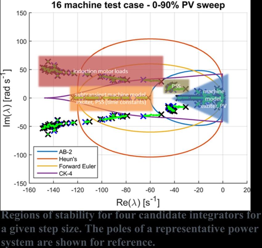
6/14
 Current Practice: Runge-Kutta Method
 The second-order Runge-Kutta (RK2) method is one of the
 most widely used numerical integration schemes in existing
 commercial dynamic simulation software tools.
 Stability region of RK2 method
 h = integration time step
 ሶ = λ is system being solved

 To maintain stability, h and/or
 |Real (λ)| must remain small ➔
 computation times will be
 relatively long and/or fast
 transients will not be accurately
 captured.
 Plot from: S. Kim and T. J. Overbye, “Optimal Subinterval
 Selection Approach for Power System Transient Stability
 Simulation,” Energies, vol. 8, pp. 11871-11882, 2015.

7/14
 Variable Time Step Algorithm
• In the variable time step
 method, the time step can
 increase as fast transients
 subside; conversely, the time
 step can be reduced to
 capture fast transients.
• This permits a reduction in
 the number of necessary
 iterations, supporting the
 use of more complex
 integration schemes.
• This is accomplished
 through time step control,
 which estimates error at
 each iteration and adjusts
 the time step to meet a
 tolerance threshold.
 Plot from: R. Concepcion, M. Donnelly, R. Elliott, and J. Sanchez-Gasca, “Extended-Term Dynamic Simulations
 with High Penetrations of Photovoltaic Generation,” Sandia Technical Report, SAND2016-0065, 2016.

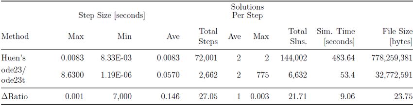
8/14
 Variable Time Step Example

 • VTS method is labeled ode23/ode23t. Simulation
 runs in PST (Matlab-based Power System Toolbox).
 • System modeled is MiniWECC: 122 buses, 171
 lines, 88 loads, 34 generators, 623 states.
 • Event is a +435 MW load step on Bus 2 at t=1 sec.
 • Each area has identical AGC that acts at t=40 sec
 and every 2 minutes thereafter.
 • Simulation is run for 10 mins (600 secs).
 • Results show VTS runs 9 times faster than FTS
 with a 24 times smaller output file size.

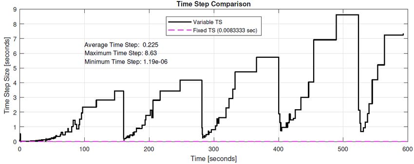
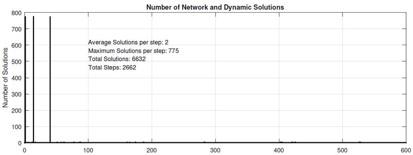
9/14 Variable Time Step Example

 Comparison of
 time step size
 for variable
 time step and
 fixed time step
 methods.

 Plot of
 number of
 network
 (algebraic)
 and dynamic
 (ODE)
 solutions for
 VTS method.

10/14 Sensitivity Analysis of VTS Method

• Model simulated in PST is Kundur 2-area 4-machine system.
• Event is a perturbation of governors to mimic solar variation due
 to cloud cover.
• Sensitivity is studied with respect to initial step size, error
 tolerance, and type of ODE solver.
• Minimal sensitivity to initial step size.
• Different error tolerances have large impact on computation time
 with minimal impact on solution accuracy.
• ODE solver type greatly impacts computation time and accuracy
 (non-stiff solvers are slower but more accurate than stiff solvers).

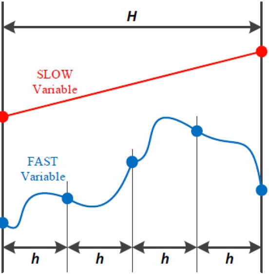
11/14
 Multi-Rate Algorithms

• Another approach to extended
 simulation times is the use of
 multi-rate methods.
• In this approach, h is a small
 timestep for fast changing variables.
• H is a longer time step for slow
 changing variables.
• H is an integer multiple of h.
• In the figure, H = 4·h.
 Plot from: S. Kim and T. J. Overbye, “Optimal Subinterval
 Selection Approach for Power System Transient Stability
 Simulation,” Energies, vol. 8, pp. 11871-11882, 2015.

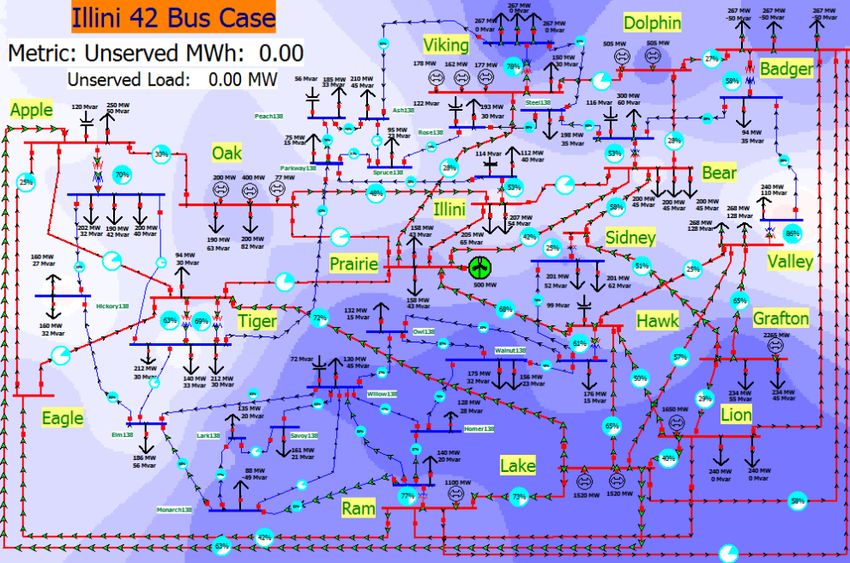
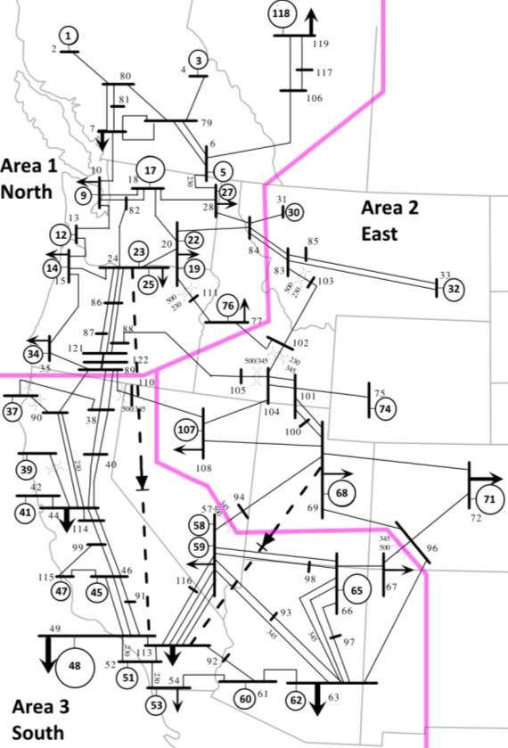
12/14 Multi-Rate Method Examples
42-bus synthetic grid for central Illinois
 2000-bus synthetic
 grid for ERCOT

 Computation times by integration
 method (simulated in PowerWorld)
 System Single Rate Reduced Multirate Larger
 Time Step Time Step
 42-Bus 2.02 s 0.24 s
 2000-Bus 147.95 s 17.52 s

 Mean squared error estimates by
 integration method MR method yields:
 System Single Rate Larger Multirate Larger
 Time Step Time Step • More accurate results
 42-Bus Does Not Converge 7.60E-7
 2000-Bus Rotor Angle 39.27 2.98E-7 • Approx. 9 times faster run times
2000-Bus Voltage Mag. 0.003 0
2000-Bus Voltage Angle 130.86 2.14E-7 • Better convergence than FTS

13/14
 Other Approaches Being Investigated

 • Parallelization techniques based on distributed computing
 to speed numerical solution of system equations.
 • Improved error analysis of numerical methods to study
 systems with noise and modeling uncertainties ➔
 uncertainty propagation.
 • Improved modeling – AGC, grid forming and grid
 following inverters.
 • Adaptive modeling framework – software that switches
 between classical transient simulation and long-term time
 sequenced power flow simulation.

14/14
 Conclusions
• Rapidly increasing grid integration of IBRs is highlighting the need for
 numerical solvers better suited to simulate the fast and slow dynamics
 associated with inverter-based resources over extended time frames.
• Existing simulation toolsets were not designed to study these vastly
 different dynamic phenomena in a single simulation scenario.
• New numerical methods, improved models, and advanced software
 techniques are being developed to address the need for longer simulation
 times of systems with dynamics on widely varying time scales.
• Project has implemented these methods and models on realistic large-
 scale grid examples using two different platforms: PST (Matlab-based
 public-domain open-source software) and PowerWorld (Commercial
 simulation software environment).