Irish Property Price Estimation Using A Flexible Geo-spatial Smoothing Approach: What is the Impact of an Address?
←
→
Page content transcription
If your browser does not render page correctly, please read the page content below

Irish Property Price Estimation Using A Flexible Geo-spatial Smoothing
                                           Approach: What is the Impact of an Address?

                                           Aoife K. Hurley · James Sweeney

                                           20 August 2021
arXiv:2108.09175v1 [stat.AP] 20 Aug 2021

                                           Abstract Accurate and efficient valuation of property is of utmost importance in a variety of settings, such as
                                           when securing mortgage finance to purchase a property, or where residential property taxes are set as a percent-
                                           age of a property’s resale value. Internationally, resale based property taxes are most common due to ease of
                                           implementation and the difficulty of establishing site values. In an Irish context, property valuations are currently
                                           based on comparison to recently sold neighbouring properties, however, this approach is limited by low property
                                           turnover. National property taxes based on property value, as opposed to site value, also act as a disincentive to im-
                                           provement works due to the ensuing increased tax burden. In this article we develop a spatial hedonic regression
                                           model to separate the spatial and non-spatial contributions of property features to resale value. We mitigate the
                                           issue of low property turnover through geographic correlation, borrowing information across multiple property
                                           types and finishes. We investigate the impact of address mislabelling on predictive performance, where vendors
                                           erroneously supply a more affluent postcode, and evaluate the contribution of improvement works to increased
                                           values. Our flexible geo-spatial model outperforms all competitors across a number of different evaluation met-
                                           rics, including the accuracy of both price prediction and associated uncertainty intervals. While our models are
                                           applied in an Irish context, the ability to accurately value properties in markets with low property turnover and to
                                           quantify the value contributions of specific property features has widespread application. The ability to separate
                                           spatial and non-spatial contributions to a property’s value also provides an avenue to site-value based property
                                           taxes.
                                           Keywords House Prices · Automatic Valuation Models · Spatial Models · Generalised Additive Models ·
                                           Hedonic Regression · Non-linear Smoothing

                                           1 Introduction

                                           There is substantial public and commercial interest in accurate and efficient automated approaches to property
                                           valuation. The purchase of a property is typically the largest lifetime financial outlay for most households and
                                           so there is an intrinsic interest in accurate estimation of the value of owned, or prospectively owned, property.
                                           From a debt financing perspective, property valuations are typically required by banking institutions to secure
                                           mortgage finance prior to property purchase, or when refinancing an existing loan. Similarly, an investment fund,
                                           bank or government agency may require regular valuations of assets under their ownership for financial reporting
                                           reasons. The price of a property will depend on a wide variety of factors, ranging from property specific features
                                           such as its type, size, quality of finish, in addition to its location in terms of proximity to schools and public
                                           transport services. However, the contribution and importance of each of these individual aspects to the value of a
                                           property will vary from country to country depending on national preferences.
                                                The valuation of properties is also of substantial governmental interest in terms of revenue generation via
                                           property taxes. In Ireland, as in a number of countries, property taxes are based on the value of the property
                                           itself, as opposed to a tax on its location or site value (Blöchliger and Kim (2016)). This method of taxation is

                                           A.K. Hurley
                                           Department of Mathematics and Statistics, University of Limerick, Limerick, Ireland V94 T9PX
                                           E-mail: Aoife.Hurley@ul.ie
                                           J. Sweeney
                                           Department of Mathematics and Statistics, University of Limerick, Limerick, Ireland V94 T9PX
2                                                                                      Aoife K. Hurley, James Sweeney

primarily due to the ease in estimating property resale values. It can, however, act as a deterrent in undertaking
improvement works that increase property values, due to the resulting increased tax. This has wider societal
impacts in areas such as climate, with energy inefficient homes substantially contributing to greenhouse gas
emissions - the residential sector accounted for 27% of all energy usage in Ireland in 2020. There is also an
incentive to mitigate the tax penalty through under-utilisation by letting a property fall into disrepair and thus
having a lower value. On the other hand, a site value tax (SVT), which does not penalise improvement works,
requires the separation of a property’s value into the constituent parts of building value and the value of the
underlying site. This site value is derived from its location and access to services, facilities and utilities. Moves
towards a full site value tax (SVT) are impeded by the difficulty in valuing land - only 3 OECD members (Sweden,
Estonia and Australia) have a tax of this form (Blöchliger and Kim (2016)).
     Automated valuation models (AVMs) provide an efficient approach to large scale property valuations, being
based on statistical models, with price prediction models constructed for several major cities worldwide. They
have substantial potential in the context of property tax calculations for property owners, due to their provid-
ing objective property valuations. AVMs can be broadly separated into two approaches at present, comprising
approaches focused on either hedonic geospatial regression modelling approaches, or alternatively taking a a ma-
chine learning perspective. The primary benefit of a spatial hedonic modelling approach is the benefit of insights
into the contribution of repective property features to price. Gelfand et al. (2007) provide a geo-spatial model
with repeat sale measures for price prediction of condominiums in Singapore. Liu (2013) investigate the property
market of the Dutch Randstad region with property variables including property type, age and size. Oust et al.
(2020) account for repeat sales as well as some property specific attributes including floor area, construction year
and garden access in an application to the Oslo housing market. In each case, the authors have access to large data
sets ranging from 16,000 to 438,000 transactions. In contrast from an explanation perspective, machine learning
or artificial intelligence based approaches to property price prediction are typically more focused on predictive
error as opposed to explainability of models. The drawback for many of the more complex approaches, such
as neural networks, is the difficulty in interpreting the relationship between selling price and house features, in
addition to the volume of data required to accurately fit models. Ho et al. (2021) apply support vector regression,
random forest and gradient boosting machine to a Hong Kong data set containing 39,554 housing transactions.
Their best model has an R2 of 90% though they report high bias in the model predictions for extreme values.
Phan (2018) evaluates the performance of various machine learning algorithms, including regression trees and
neural networks to the Melbourne property market noting difficulties in the interpretation of the prediction output
and over-fitting issues. In general, machine learning approaches require substantial data sets to train models, with
overfitting an issue in smaller ones. It is not clear that the methods would have similar accuracy results in areas
with much lower property turnover.
     In this article, we focus on the development of geo-spatial statistical models that have improved price predic-
tion performance and interpretation for small data sets in regions where property transactions are low or relatively
infrequent. We explore the impact of address mislabelling and allow for public bias in postcode allocation in the
Dublin market, where property addresses are misreported. Our focus is on explaining the contribution of each
property component to overall price - we evaluate the impact of improvement measures such as improved energy
efficiency or renovation, on the value of a property, allowing for a deeper understanding of the contribution and
dominance of property specific aspects on value. Finally, we provide a speculative framework using estimated
land values for the development of a land value based tax system in an Irish context which may allow for a more
equitable distribution of property taxes. A key benefit of our model-based approach is the accounting for uncer-
tainty in model parameters in ensuing price prediction intervals - machine learning algorithms by default usually
provide point estimates only, and so decisions are made ignoring the uncertainty surrounding these estimates.
     Our article is organised as follows. In Section 2 we introduce our data set for the Dublin property market
and provide an exploratory analysis of the links between spatial location and property features with price. In
Section 3 we outline our statistical modelling methodology and we outline our models and selections required
for a Gaussian Process smooth. Section 4 presents the results, while the final section concludes the article.

2 The Irish Property Market

Irish people have historically had a strong preference for home ownership over renting, with a home ownership
rate of 70.3% in 2018 (Eurostat (2018)). In most cases, properties are sold by private treaty. Bidders submit their
offers to the selling agent who liaises with the vendor, with the property typically sold to the highest bidder.
On average only 2% of properties change hands per year, with the average house transacted approximately once
every 60 years (Maguire et al. (2016)). For property valuations, property agents base estimates on a combination
of their opinion and prices of similar nearby sold properties. This approach suffers from a number of deficits.
First, due to low property turnover, the number of nearby comparison properties is typically low. The comparison
What is the Impact of an Address?                                                                                   3

properties may also be of a completely different type, for example apartments as opposed to houses. Second, the
Irish residential property price register only includes date of sale, price and address, and does not provide property
specific information. Consequently, there can be a large degree of variation in estimates from a nearest neighbours
type approach. Due to these issues, there has been little to no progress in the development of automated property
valuation models (AVMs) for Ireland.

    Within Ireland, the Dublin property market accounts for approximately one third of all property transactions
and provides the focus for this article. The county of Dublin has 25 postcode regions shown in Figure 1, with
a breakdown of the median property price per postcode region. For clarity, postcodes have been shortened from
Dublin X to DX. The river Liffey bisects the city into north and south - for numbered postcodes, the even numbers
are south of the river and odd numbers are to the north. Though a generalisation, postcodes in the south-east of
the city and south county are perceived to be the more affluent areas with the north inner city areas seen to be
more economically deprived (Kelly and Teljeur (2007)). There has long been speculation that people would pay
more to have a perceived affluent postcode on their address.

                                         Fig. 1: Median price per postcode
4                                                                                           Aoife K. Hurley, James Sweeney

2.1 The Dublin House Price data set

Properties that are for sale are typically listed on at least one of a number of online property portals, with Daft.ie
and MyHome.ie the largest providers on the Irish market. The data set available for exploration and model de-
velopment was provided by 4Property Ltd, containing property sales in Dublin (both city and county) for dates
between January 2018 and November 2018 inclusive, amounting to 5,285 transactions in total. This was reduced
to 5,208 properties after removing properties with incorrect information such as size, or with floor areas below
minimum size thresholds of 37m2 . In Table 1 we have listed the data fields provided with each property. The ‘De-
scription’ variable includes detailed extensive descriptive information on individual properties that is, to the best
of our knowledge, not available to historical researchers, particularly in an Irish context. At the property level,
the description typically includes details on features such as property aspect, heating systems used and general
property condition. In Section 2.2 we outline our approach for mining the description for key words speculated
to be influential in previously published research or via expert opinion on influential property variables. Unlike
other major cities worldwide, age does not play a major role when advertising properties in Dublin. Parts of the
city were developed at different times and so building stock and its age may be loosely associated with postcodes
that have been developed at different times. Energy rating is sometimes also a proxy for age with newer dwellings
having much higher energy ratings than historic stock.

                      Variable         Description
                      Price            Sale price of property in C
                      Sale Date        Date the property was sold
                      Latitude         Latitude co-ordinate of the property
                      Longitude        Longitude co-ordinate of the property
                      Neighbourhood    Townland, village or town in which the property
                                       is located
                      Baths            Number of baths in the property
                      Beds             Number of beds in the property
                      BER              Building Energy Rating (BER) for the property, properties
                                       less than 50m2 are exempt - are not required to have a rating
                      Description      A written description that was used
                                       in the advertising of the property
                      Size             The floor area of the property in m2
                      Property Type    Classification of property type,
                                       e.g. Duplex, End of Terrace House, Semi-Detached House, etc.
                      Postcode         Original postcode provided by the vendor for the property

                                          Table 1: Description of Data Set

     The mean sale price for the 5,208 properties sold between January 2018 and November 2018 is C484,443,
with the median price of C392,000, highlighting the skewed nature of property prices in the data set. We alleviate
this issue by standardising price by floor area, resulting in a mean and median prices per m2 of C4,569 and C4,405
respectively. There is little variation in size across the 25 postcodes. In Figure 2 we provide a breakdown of the
price per m2 by postcode. Within postcodes, the distribution of price per m2 is broadly symmetric. We notice a
higher degree of variability in postcodes that have span large areas and have a diverse range of people of differing
socioeconomic backgrounds. One example of increased variability is seen in Dublin 4 which encompasses a large
area with various levels of affluence, and subsequently has a broad interquartile range, as well as having multiple
outliers. This is unlike Dublin 20, which covers a small area with little variation in socioeconomic backgrounds
and this is seen in the variation in price per m2 . The ordering of the postcodes is both alphabetical and can be
coarsely equated to distance from the city centre. We would expect price per m2 to reduce with increased distance,
however, D14 and D16 have higher medians as compared to postcodes of a comparable distance from the center
of the city. This could be down to many reasons including the light rail system (LUAS) servicing these postcodes
providing a sought-after link with the city centre. Alternatively the impact could be for socioeconomic reasons
with these postcodes having an increased valuation for perceptions of affluence.
    In Table 2 we provide an overview of the number of properties and pricing information for each property
type and within each postcode. For some postcodes, such as Dublin 10 and Dublin 17, we witness extremely
low property turnover, which would pose problems for nearest neighbour based methods. The table also provides
details of the breakdown of properties by type. We observe the dominance of certain property types within post-
codes, e.g. D1 and apartments, and others have a broad mix, e.g. North County Dublin. When there is a dominant
property within a postcode, valuations of other property types within that postcode is difficult.
What is the Impact of an Address?                                                                                  5

                                       Fig. 2: Variation in sale price per m2

     In Figure 1 we present the median price of properties within each postcode, averaged over dwelling type and
size. We observe a spatial pattern that has higher median prices clustered together in the south city along the coast
and lower median prices along the north and west county border. In Figure 3 we visualise the spatial structure
in price per m2 across Dublin. To do so, we create 14 groups of approximately equal size and group based on
observed price per m2 values. These groupings make clear the variation in prices across the county of Dublin and
is robust to outliers in the data. Similar to Figure 1, higher values (dark red) are concentrated together around the
city centre, to the south of the city and along the coast. Lower values, shown in dark green, are observed as one
moves away from the city centre towards the county border.

2.2 Text Mining of Price Prediction Features

Valuable information is contained in the textual summary of a property, requiring the use of natural language
processing tools to extract features of interest. There is some published research identifying such features: Rosiers
et al. (2007) and Mayor et al. (2009) explore the impact of gardens on price with an increase in explanatory
performance of their models and reduced prediction error. Lu (2018) found that dwelling units with southerly
aspects have higher property value in an examination of the Shanghai housing market. Abdulai and Owusu-Ansah
(2011) noted the improved predictive performance of models for the Liverpool housing market with the inclusion
of garage, garden and central heating. Asabere (1990) ventures that there is a premium for having a property on
a cul de sac. Kiefer (2011) include a variable for fireplace in their models and notes the positive impact on price.
Oust et al. (2020) include the variables ‘penthouse’, and ‘garden’ amongst others in their models. Several articles,
including van Ommeren et al. (2011), investigate the impacts of parking policy on house prices. Wittowsky et
al. (2020) construct an ordinary least squares (hedonic) model and a spatial lag model to investigate the impact
of different attributes including accessibility, ‘walk score’ and socioeconomic characteristic of neighbours on
residential housing prices. However, the lack of demographic information at the household level in an Irish
context means that such variables cannot be included.
     We performed a simple, case insensitive string search for certain housing characteristics with the descriptive
phrases identified driven by previous literature as well as expert opinion on features of specific interest in an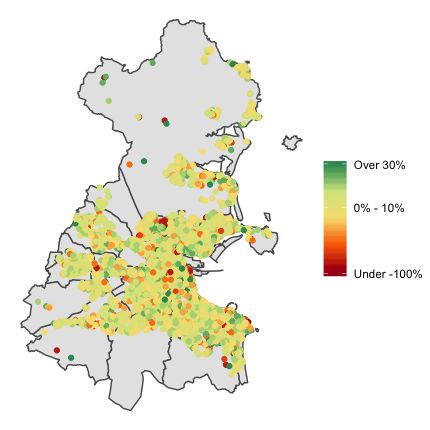
6                                                                                                        Aoife K. Hurley, James Sweeney

    Postcode              Apartment   Detached   Duplex      End of       Semi-Detached   Terraced   Townhouse   Number of    Median Price
                                       House              Terrace House      House         House                 Properties     per m2
    D1                      51            0        1            2                0             7        0           61          C4,869
    D2                       45           0         0            1               1             5        2           54          C6,641
    D3                       27           9         0           21              33            62        0           152         C5,117
    D4                       72          22         3           20              38            73        8           236         C6,753
    D5                       10          12         3           26              82            59        0           192         C4,118
    D6                       39          15         3           19              36            60        5           177         C6,481
    D6W                      17          11         1           10              57            22        0           118         C5,112
    D7                       38           7         4           32              23           107        0           211         C4,857
    D8                      117           1         5           26               7           112        4           272         C5,064
    D9                       53           9         3           23             101            59        2           250         C4,166
    D10                       5           2         0            9               0            14        0           30          C2,962
    D11                      28           4         2           15              35            39        2           125         C3,136
    D12                       7          10         0           45              35            86        0           183         C3,971
    D13                      24          15         6           15              45            30        0           135         C3,790
    D14                      26          25         1           12              93            39        4           200         C5,337
    D15                      74          46        22           20             117            32        2           313         C3,231
    D16                      32          19         1            6             115             7        2           182         C4,553
    D17                      13           3         1            2               8             4        0           31          C3,190
    D18                      76          60         4            9              59            14        4           226         C4,503
    D20                       5           1         1            1               8             8        0           24          C3,571
    D22                      14           7         2            7              30            18        0           78          C2,937
    D24                      34           7         4           17              37            28        2           129         C3,093
    NCD                     145         107        34           63             176           129        7           661         C3,441
    SCD                     209         140        21           42             267           128        8           815         C5,350
    WCD                      58          21        12           18             132            36        5           282         C3,088
    Dublin County            31          14         5            5               8             8        0           71          C3,875
    Total                  1,250        567       139          466            1,543         1,186      57          5,208        C4,405
    Median Price per m2    C4,573      C4,743    C3,096       C4,150         C4,320        C4,389     C5,078

                              Table 2: Number of Properties and Median Price per m2 per Postcode

Irish context. The plot or site size is an obvious important variable in the valuation of a property, however this
information is not explicitly available with each transaction listing. Only 172 properties (3% of data) mentioned
“acre” in their description. In addition, the average plot size in Dublin varies by postcode and is not easily ob-
tained. We attempt to identify a proxy for this variable by identifying properties where development potential or
large gardens are prominent within textual descriptions. In Table 3 we list the words and phrases mined within
each textual description in addition to their numbers of occurrence. In addition to these variables, ‘Attic Conver-
sion’, ‘Development Potential’, ‘Open Plan’, ‘Immersion’ and ‘Hot Press’ were identified. Converting attics into
another living space to increase available floor area is becoming more common in the Irish property market due
to the reduced cost in comparison to an increase in property footprint. A property with development potential
for an extension would generally sell for more with the opportunity for the buyer to increase property size or
build additional units on the site. Open plan living spaces are also extremely popular at present. ‘Immersion’ is a
reference to water heating being electric and thus more expensive typically. Due to the proportion of rainy days
in Ireland access to an airing closet is preferred for clothes drying, resulting in the inclusion of ‘hot press’.

                                       Word or Phrase(s)                     Number of Observations
                                       South Facing or South Orientation              871
                                       Attic Conversion                               190
                                       Parking or Car Spot/Space                     3782
                                       Development Potential                          492
                                       Open Plan                                     1512
                                       Fireplace                                     2403
                                       Central Heating                               2596
                                       Immersion                                      196
                                       Hot Press                                      993
                                       Garage                                         770
                                       Large Garden                                   155
                                       Ground Floor Apartment                         201
                                       First Floor Apartment                          119
                                       Second Floor Apartment                          66
                                       Penthouse Apartment                             39
                                       Refurbished/Renovated/Upgraded                1219
                                       Cul-de-Sac                                    1006

                                      Table 3: Attributes Extracted from ‘Description’ variable

    Most hedonic regression models contain some distance measures as a proxy for spatial location, such as to
the Central Business District (CBD). We construct similar variables with distance measures calculated as the
shortest distance between two points on an ellipsoid. We assign the International Financial Services Centre, or
What is the Impact of an Address? 7
Fig. 3: Price per m2
IFSC, as Dublin’s CBD. We also construct a number of categorical indicator distance variables with the distance
tapered to have zero affect above a distance threshold. These include indicator variables for proximity to parks,
transport hubs and the city center - the distance measures taken and the radius distance are presented in Table 4.
Additionally, interactions terms for ‘Garden’ and ‘Parking’ within city centre areas were taken. This is due to the
high demand for parking and gardens within the city centre for a 2km radius, which we believe would add value
and reduce modelling errors. Properties outside the city centre typically have free parking and garden access and
so these aspects would not add to their value.
Location Maximum Distance Data Type
International Financial Services Centre (IFSC) NA Continuous
Dublin Airport 5KM Categorical
O’Connell Bridge (City Centre) 2KM Categorical
Dublin Area Rapid Transit (DART) Station 1.5KM Categorical
LUAS (Light Rail) Stop 1KM Categorical
Park or Public Green 5KM Categorical
Table 4: Distance Measures8 Aoife K. Hurley, James Sweeney
3 Automated Valuation Models
In this section we introduce the suite of models we apply to the data set in order of complexity including; classic
hedonic regression, a nearest-neighbours based approach and geo-spatial based models.
3.1 Hedonic Regression
Forms of hedonic regression are used throughout the literature for property price prediction, generally as a base-
line model as a comparison to recent modelling advances. Oust et al. (2020) use hedonic models that have ad-
ditional terms that combine single and repeat sale measures and compare these to their geographically weighted
regression approach. Lu (2018) construct a hedonic pricing model for the Shanghai housing market in order to
estimate the impact of property aspect. Similarly, Mayor et al. (2009) use a hedonic house price model to estimate
the effects of green spaces on property prices.
Our hedonic regression model takes the form
loge (Vi ) = β0 + ∑ Xki βk + ∑ Zli γl + εi (1)
k l
where Vi represents the price per m2 of property i and εi ∼ N (0, σ 2 ) is iid unstructured Gaussian noise. It
is typical to model log price per m2 , being less affected by the skewness introduced by the right tailed nature
of house prices in comparison to a lower price bound at 0. Our model is specified as follows: β0 is an intercept
term relating to the mean log(price) per m2 . We group the property characteristics into continuous effects Xi =
{sizei , bedsi , bathsi , CBDi }, and dummy (or intercept) indicator labels Zi comprised of the features outlined in
Table 3 in addition to property postcode, property type and energy rating. βk and γl represent the regression
scaling coefficients associated with variables Xk and Zl respectively. These models are easy to fit using standard
least squares or maximum likelihood methods, and their properties are well known. Spatial aspects in the data set
are coarsely modelled through the postcode indicator variables and the distance measures for proximity to parks
and transport services. As we will observe in later sections, this model is not sufficiently complex to account for
non-linear structured patterns in some of the model variables as well as the distance measures.
3.2 Machine Learning Based Approaches
The most prevalent approach to valuation in an Irish context is a form of k-nearest neighbours averaging, as
outlined in Algorithm 1. In order to control for the effect of property type, we group comparison properties by
type to ensure that the neighbours identified for each property are the same. We also control for the impact of
property size by basing estimates on the price per m2 of neighbouring properties as opposed to raw price alone.
Algorithm 1 Nearest Neighbours Approach
1: for i = 1, . . . , 5208 do
2: for k = 3, 5, 7, 9 do
3: Create subset of data set of type property i, Y (i) .
(i) (i)
4: Identify set {y1 , . . . , yk } of the k spatially nearest neighbours to property i
(i) (i)
5: Estimate price per m2 as ỹi = median{y1 , . . . , yk }
6: Y
ei
return K nearest neighbour estimates {Y
e i , 1, . . . , 5208}
The major strength of this approach is the ability to incorporate spatial correlation in predictions in terms
of location and postcode by utilising neighbouring properties. We also control for two of the primary value
driving features in property type and size. However, the accuracy of this approach is greatly affected by a lack
of neighbouring comparable properties, in addition to not controlling for the characteristics of these properties.
As outlined in Table 2, the property types in a locality can be quite heterogeneous in nature and we observe the
impact of this in the accuracy of price predictions using this method in Section 4. In Section 6 we discuss the
performance of a more complex decision tree and random forest approaches to model fit. The primary issue in the
applications of these models in an Irish context is the lack of sufficient data to train models, particularly outside
of large urban areas.What is the Impact of an Address? 9
3.3 Geo-spatial Modelling
The primary benefit of a geo-spatial approach to property price prediction is that it enables the reduction of un-
certainty in areas with low numbers of property transactions. This is achieved by leveraging information from
neighbouring areas where there is more data to give more certainty in predictions for areas with less data. Basu
and Thibodeau (1998) examine the spatial autocorrelation in a data set of over 5000 transactions of single-family
homes in Dallas, Texas. They propose that adjacent properties might have similar observable and unobservable
characteristics resulting in properties in close proximity being similarly priced. Farber and Yeates (2006) com-
pare four models on 19,007 housing sales in Canada. These comprise: an ordinary least squares model, a spatial
autoregressive regression model, a geographically weighted regression (GWR) model and a moving window
regression model. They report the GWR model as obtaining the highest R2 , but the authors do note some disad-
vantages to GWR including irrational coefficients. Gao et al. (2006) propose an alternative way of empirically
evaluating models, using house and land price data set in Tokyo from Gao and Asami (2001) concluding that if a
spatial relationship is implied in the data, spatial models outperform a simpler model. Gelfand et al. (2004) use a
Gaussian process based approach to model spatial correlation in a Louisiana housing data set noting that spatial
effects emerge as very important in explaining house prices. Bourassa et al. (2007) implement both Conditional
Autoregressive (CAR) and Simultaneous Autoregressive (SAR) models, as well as other geostatistical models, to
a data set containing 4,800 transactions for Auckland, New Zealand. They find that the CAR and SAR methods
perform poorly when compared to they other geo-statistical models they fit. Liu (2013) compare the prediction
performance of a spatiotemporal autoregressive model to a traditional hedonic model. The analysis is performed
on a comprehensive housing transaction data set from the Dutch Randstad region, which spans ten years, 1997
to 2007 with 437,734 transactions. The data set contains variables on both structural attributes and the region or
submarket the house is located. This article found that spatial dependence was of a larger magnitude than that
of temporal dependence. Liu concluded that accounting for spatial and temporal dependence is not only theoret-
ically warranted, but contributes to better prediction performance. Ahrens and Lyons (2021) construct a model
linking commuting times to rental prices in the Dublin region, with rising rents linked to shorter commuting times
showing the importance of spatial proximity in valuation models. Lyons (2019) explores the relationship between
the advertised asking price for dwellings that are listed on estate agent platforms and final sale prices, showing
they act as a good proxy. However, no property level data in terms of descriptive features are used. Oust et al.
(2020) apply a number of spatial modelling techniques to a Norwegian property data set. They use regression
kriging and GWR among other models for modelling the spatial component. The best performing model they
fit was a GWR model that included measures of repeat sales. By including the repeat sales, they increase their
median absolute percentage error from 6.65% to 6.20%.
In the remainder of the section, we present our spatial modelling approach.
3.3.1 Generalised Additive Models
A Generalised Additive Model, or GAM, is a non-parametric extension of generalised linear models (GLM) with
the linear predictor involving a sum of smooth function of covariates (Wood (2017)). The primary benefit of a
GAM based approach over linear models is the flexibility of modelling non-linear relationships between predictor
variables and the response, in addition to the interpretability of a standard linear model. Smoothing splines are
typically used to model non-linear univariate or bivariate relationships between variables and provide a way to
smoothly interpolate between points. Splines allow for a certain degree of localised flexibility, in contrast to
the the use of higher degree polynomials that would lead to undesirable global effects. Spatial GAMs are most
commonly used in climate applications due to their computational advantages in modelling large spatio-temporal
data sets, for example in the modelling of air pollution, (Ramsay et al. (2003) and Wood et al. (2017)), and
problems associated with fisheries (Wood and Augustin (2002)). There has been limited application in the area
of property modelling - GAMs were used by Panduro and Veie (2013) in estimating the effect of green spaces on
house prices.
GAMs, in a Gaussian context, have the form
loge (Vi ) =β0 + ∑ Xki βk + ∑ Zli γl + f1 (Bedsi ; k1 )+
k l
f2 (Bathsi ; k1 ) + f3 (CBDi ; k2 )+ (2)
f3 (Sizei ; k2 ) + f4 (s1i , s2i ; k3 ) + εi
where loge (Vi ) is the log price per m2 , and Z, β and γ are as in Equation 3.1. For ‘Type’, ‘BER’ and ‘Postcode’
we impose a sum to zero constraint with coefficients within each variable relative to the grand mean rather than
a base line category, increasing the interpretability of our outputs.10 Aoife K. Hurley, James Sweeney
As opposed to being modelled linearly via X previously, CBD distance and property size are modelled via
smoothing splines, f j (Wood (2017)). For the 1-D splines, we use cubic regression splines with 5 knots for beds
and baths, and 20 knots for size and IFSC distance, equally spaced across covariate quantiles. They are penalized
for smoothness using conventional integrated square second derivative cubic spline penalties (Wood (2017)).
We convert the longitude and latitude recordings to Cartesian coordinates and specify a Gaussian process for
the spatial relationship. This requires the specification of a smoothing kernel for the covariance function, based
on Euclidean distance between observations. We specify one proposed by Kammann and Wand (2003),
|r| |r|
Cθ (r) = σx2 1 + exp − (3)
ρ ρ
as this requires only one parameter to be estimated in comparison to spherical and Matérn function approaches.
We observed negligible differences in the estimated spatial fields when using this simplified covariance function
as compared to more complicated members of the Matern covariance class.
Models are fit using the mgcv package within the R programming language. A penalized maximum likelihood
approach is used in fitting models with smoothness penalties on each of the spline parameters. Models were fit
with several different choices of the the number of knots for each smoothing spline to determine sensitivity of
results to this parameter, which lead to 100 knots for the geo-additive term and is discussed further in Section 4.1.
We fit four different GAM models with the differences between them outlined in Table 5, with more model detail
provided in Table 11.
GAM Includes
1 Linear and smooths, distance variables, no spatial component
2 Linear for all variables, distance variables, spatial component
3 Linear and smooths, no distance variables, spatial component
4 Linear and smooths, distance variables, spatial component
Table 5: GAM Models
4 Results
For our preliminary models, we used the postcode provided with each property listing. We investigate the impact
of address misspecification and resulting bias in Section 4.4. For variable selection we follow the approach of
Gelman and Hill (2007, Section 4.6): if a predictor has the expected sign it is retained in the model whether
statistically significant or not, otherwise further analysis is carried out on the variable itself to determine its
exclusion. We use 5-fold cross validation for model comparison. The accuracy metrics for model comparison
are: the prediction intervals; median error percentage; R2 and root mean squared error (RMSE).
4.1 Selecting the optimal number of knots for the spatial surface
We determine the number of knots required by running the models for increasing knot values and identifying
an ‘elbow’ in the plot of k versus accuracy measures. Figure 4 shows these plots for GAM 3. From left to
right the columns show: R2 against k; RMSE against k and 95% predictive interval coverage against k. The
prediction intervals measure the uncertainty associated with a price prediction, and enable evaluation of statistical
distribution assumptions. Ideally k is as low as possible for computational reasons, but with a requirement to retain
satisfactory accuracy statistics - the higher the value of k, the longer the models take to fit. From these plots, we
highlight the selected value of k = 100 for our spatial surface.
4.2 Fitted Models and Interpretation
Table 6 presents accuracy estimates for the county of Dublin. These accuracy estimates include median absolute
percentage error, percentage of predictions within 10% of sale price and a number of prediction intervals. We
notice higher percentage coverage than expected in the prediction intervals for the linear and GAM 2 models.
One reason for this could be the models are not describing the data well, which results with an increase in theWhat is the Impact of an Address? 11
Fig. 4: Estimates of R2 , RMSE and prediction interval coverage for increasing number of spatial knots.
error variance parameter and thus the prediction intervals are compensating. As house prices are spatially auto-
correlated (Basu and Thibodeau (1998)), residuals of models that do not include a spatial element may retain
this. Moran’s I is a measure of spatial autocorrelation, and is shown for every model in Table 6. Moran’s I ranges
in values from -1 to 1, with 0 indicating no autocorrelation. Table 6 illustrates Moran’s I approaching 0 with
increasing model complexity.
Model R2 RMSE Median Absolute Within 10% Within 20% In 50% Predictive In 95% Predictive Moran’s
% Error of Price of Price Interval Interval I
Basic Linear Model 0.73 C182,508 18.32% 28.25% 54.17% 49.7% 94.9% 0.117
Linear Model 0.81 C154,160 12.10% 42.99% 72.08% 54.2% 94.6% 0.029
GAM 1 0.85 C132,758 11.22% 45.81% 75.52% 47.0% 93.1% 0.025
GAM 2 0.83 C146,421 9.67% 51.75% 81.59% 52.2% 94.8% 0.010
GAM 3 0.87 C123,448 8.57% 56.37% 84.95% 48.3% 93.9% 0.009
GAM 4 0.87 C123,639 8.50% 56.37% 84.98% 48.5% 93.9% 0.008
Table 6: Accuracy Statistics from 5 Fold Cross Validation
Our optimal model is GAM3 which includes a spatial surface, smooths applied to ‘Size’, ‘No. Beds’ and ‘No.
Baths’ along with binary variables and no distance metrics, i.e. distance to the Airport and CBD are excluded. We
select GAM 3 to be our best model as excluding the distance metrics enhances the interpretability of the spatial
surface. GAM 3 has the lowest RMSE shown in Table 6, and has the same values as the GAM 4 model in other
measures.
For GAM 3 we examine the accuracy for closed interval subsets of the data (e.g. between C450,001 and
C500,000) and the cumulative median absolute percentage error in Table 12. We note that our accuracy mea-
sures remain relatively constant up to the interval C650,001 to C700,000, which when examined cumulatively,
accounts for 81.9% of our data. Up to this interval, the cumulative median absolute percentage error is 8.03%,
0.54% lower than the overall median absolute percentage error. Within some intervals, the median absolute per-
centage error is below 8% (7.25% between C300,001 and C350,000; 7.95% between C350,001 and C400,000;
7.68% between C500,001 and C550,000; 7.31% between C600,001 and C650,000). Within Table 12 the num-
ber of properties within each interval is shown, indicating that larger numbers of properties does not necessarily
translate into improved predictions.
We note the reducing spatial autocorrelation in the residuals of the models that include a spatial surface
compared to those that do not. Figure 5a shows the residuals spatially plotted for the GAM 3 model, which echos
the Moran’s I statistics that there is little spatial autocorrelation remaining. The percentage errors from the linear
model (Figure 12a) retains a certain degree of spatial structure. We see this with the clustering of similar colours
(e.g. dark green in the north east coast), which is less evident for the GAM 3 model (Figure 12b).
Although our models give good accuracy measures, there is evidence of heteroscedasticity shown in Fig-
ure 5b. This is clearly evident in properties that have sold for over C1,000,000. Approximately 5% of our data set
have sale prices over C1,000,000 and this reduces the over all accuracy measures of our models. Figure 5b echos
our findings from Table 12 in which the median absolute percentage error increases substantially for properties
with a sales price of C1,000,000 or more, decreasing our predictive performance and increasing the variability in
these predictions.12 Aoife K. Hurley, James Sweeney
(b) Predicted price against Actual price. Increase in variability
(a) Residuals from 5-fold Cross Validation
with increasing price
Fig. 5: Visualising results of GAM 3 model
Interpretation of Coefficients In the following we focus on the outputs of the GAM3 model. The model parameter
coefficients are relative scalings. For categorical variables, rather than being compared to a base category we
constrain with respect to to the overall grand mean across levels within the variable. The coefficients can be
observed in Figure 6, where the linear coefficients are broken into three plots, showcasing the coefficients for
‘Type’, ‘BER’ and ‘Binary Variables’ separately. Table 13 gives the estimated coefficients and their associated
95% confidence intervals. In Figure 6 and Table 13, a relative scaling of 1 indicates no impact from that variable, a
relative scaling less than 1 shows a reduction in value and greater than 1 an increase in value. To aid visualisation
in Figure 6, a relative scaling of 1 is highlighted by a grey dashed line.
These plots enable us to create a hierarchy of property types and BERs. This helps when quantifying the
additional premiums associated between different categories of these variables. This enables us to assess the
premiums for various combinations, not just relative to a base line category. For example, we estimate that a
detached house has a coefficient value between 1.15 and 1.18, with mean 1.16, and a semi-detached house has
a coefficient value between 1.10 and 1.13 with mean 1.11. Consequently this would indicate that the premium
1.11
for a detached house over a semi-detached equivalent would be 4% (1 − 1.16 ). Since our coefficients are relative
0.88
scalings, we can also calculate the premium for an apartment over a duplex equivalent to be 3% (1− 0.91 ). Similar
calculations for comparisons can be made for BER ratings - upgrading a property from a G rating to an A rating
increases the value by 13% (1 − 0.94 1.08 ). We also estimate the premium for a renovated property to be between
3% and 5% over a non-renovated equivalent. In our model we include both the ‘Car Space’ and ‘Car Space.CC’
terms, and although the coefficient of ‘Car Space’ is 1, implying no impact, ‘Car Space.CC’ has a coefficient of
1.04 signifying an additional 4% premium for properties with a car parking within the city centre. Unsurprisingly,
having a garage adds a significant premium of between 6% and 8%. However, the largest estimated premium is
associated with ‘Penthouse Apartment’ which takes a value between 8% and 19%. From these estimates, we can
indicate to homeowners the possible additional value undertaking home improvements will add to their property.
These estimates also lend themselves to policy makers when allocating funding for people to improve their homes
energy performance or BER.
Investigating Smooths Although the coefficients of the smooths do not have the same level of interpretability as
those of the linear terms, we can visualise the smooths (Figure 7) and interpret the relationships. Starting from
the leftmost plot in Figure 7, we see that the effect of beds increase and then plateaus in value add at 4 beds. This
would imply that there is little difference in effect of additional beds after 4 however the uncertainty intervals are
large given a paucity of properties with beds of this number. The relationship between value and baths initially
increases until it reaches 2 baths, and then declines. This decline is most likely associated with old properties
than have been split into several multi-occupancy units and require large investments to bring them up to modern
standards. The most interesting relationship is perhaps between property value and size. Smaller properties, up to
150m2 , are more expensive than larger ones on a per m2 basis. The effect would appear to plateau at 200m2 , butWhat is the Impact of an Address? 13
Fig. 6: Model coefficients for GAM 3 model, linear variables divided into three groups: ‘Type’, ‘BER’ and
‘Binary Variables’
for an unexpected increase at 300m2 . Investigating the 88 properties that have sizes between 250m2 and 400m2
reveals that the majority are large Georgian or Victorian properties in extremely affluent areas of the city and
highly sought after.
Fig. 7: Visualising 1D smooths from GAM 3 model
4.3 Machine Learning Based Estimates
The nearest neighbours algorithm we implement (Algorithm 1) is on a price per m2 basis, controlling for property
size. The results of this approach are shown in Table 7.14 Aoife K. Hurley, James Sweeney
Number of Median Absolute Within 10 % Within 20 %
Neighbours % Error of Price of Price
3 11.30% 45.37% 73.91%
5 10.98% 46.47% 75.29%
7 10.95% 46.70% 75.40%
9 10.92% 46.72% 75.29%
Table 7: Accuracy statistics for nearest neighbours approach for price per m2
The statistics seen in Table 7 give similar or improved statistics compared to the linear models from Table 6,
but on a whole under-perform when compared to the more flexible GAM models. There are also indications that
increasing the number of neighbours does not necessarily mean improved accuracy.
We trained both decision tree and random forest models as an alternative. Results from the implementation
of two decision trees and two random forests are presented in Table 8. ‘Tree 1’ is a decision tree that includes all
variables apart from ‘Longitude’ and ‘Latitude’, ‘Tree 2’ is a decision tree that includes all variables including
‘Longitude’ and ‘Latitude’ and ‘Forest 1’ and ‘Forest 2’ follow the same convention.
Model R2 RMSE Median Absolute Within 5% Within 10% Within 20%
% Error of Price of Price of Price
Tree 1 0.80 C149,444 13.48% 20.22% 39.27% 67.49%
Tree 2 0.81 C148,977 13.32% 20.56% 39.13% 68.33%
Forest 1 0.87 C122,937 9.54% 28.01% 51.71% 80.07%
Forest 2 0.88 C117,328 8.82% 30.34% 55.38% 83.53%
Table 8: Results from decision tree and random forest approaches
From Table 8, we see that the random forests are marginally more accurate at predicting the mean (R2 and
RMSE) than our GAM models from Table 6, however are less accurate in prediction interval coverage. Although
we can compare the results of the random forests and GAM models, in taking a GAM approach we reap the
benefit of being able to interpret our models and can assess the impacts of specific variables.
4.4 The Impact of Address Mislabelling?
The initial analysis used the given postcodes on the property listings. However, some properties had given the
neighbouring, typically more affluent, postcode rather than their actual one. We assess the impact of postcode
misspecification by correcting the postcodes and re-running our analysis. 16% of properties in the data set (833
properties) gave the incorrect postcode in their advertisement. We investigate 15 postcode changes (outlined in
Table 9), based on a cross tabulation of the postcodes, shown in Figure 8, and prior knowledge of the Dublin
property market. In Figure 8, the white lines for D20 and D22 indicate no changes in postcode labeling was
required. In the models ‘GAM 5’ and ‘GAM 6’ in Table 10, the postcode changes are modelled by adding 15
dummy variables to previous models, one for each postcode change. GAM 5 and GAM 6 are the GAM 3 and
GAM 4 models respectively, with the postcodes corrected.
Figure 9 presents the estimates for the 15 postcode changes. The labels can be read as ‘Given Postcode.Corrected
Postcode’, e.g. “D11.D9” is a property listed as D11 but with correct postcode D9. The majority of the estimated
coefficients are positive, indicating a premium in sales price in each case where giving a neighbouring, more
affluent postcode. It is clear that “D11.D9” and “D16.D14” are different to the other changes estimated, with
scalings less than 1. These properties have listed postcodes with a lower median price (less affluent) than their
correct postcode. For properties incorrectly listing a more affluent postcode, there is evidence of an additional
premium being added to property values - for 13/16 postcode changes the mean scaling estimates are greater
than 1. The estimates have larger confidence intervals than those seen previously in Figure 6, as there are fewer
transactions to estimate from.
In Figure 10 we present the estimated scalings associated with the corrected postcodes. If the underlying
spatial surface captured all spatial structure in the data, the postcodes should be labels alone, with no obvious
patterns. However we note there is substantial evidence of a strong bias in postcode effects. The postcodes D7,
D8 and D9 have extremely significant impacts on price with these representing popular, up-and-coming areas
reflected in scaling estimates much greater than 1. D10, D22 and D24 all have scalings substantially less than 1What is the Impact of an Address? 15
Given Postcode Corrected Postcode Occurrences
Dublin 5 Dublin 13 3
Dublin 6 Dublin 6W 12
Dublin 6W Dublin 12 3
Dublin 9 Dublin 3 3
Dublin 9 Dubin 17 10
Dublin 11 Dublin 9 7
Dublin 14 Dublin 16 19
Dublin 16 Dublin 14 5
North County Dublin Dublin 15 9
South County Dublin Dublin 4 27
South County Dublin Dublin 18 101
South County Dublin Dublin 24 32
West County Dublin Dublin 15 38
West County Dublin Dublin 22 24
West County Dublin Dublin 24 45
Fig. 8: Heatmap of the changes that occur in postcodes Table 9: 15 Postcode Changes Investigated
Fig. 9: Estimates of Postcode Changes
which would suggest these areas are undervalued relative to their spatial location. This is perhaps due to negative
connotations regarding areas within these postcodes that are socially deprived and underprivileged. Table 14 lists
the mean estimate and confidence intervals for the postcodes.
Overall, there is little difference in accuracy between using given postcodes and corrected postcodes (Table 6
and Table 10). We do see improvements in the median absolute percentage error as it reduces for all models and
there is a rise in the proportions within 10% and 20% of sale price. Though we do see improvements with our
predictions when using the corrected postcodes, these improvements are relatively minor.
We can visualise and explore the Gaussian Process smooth used to model the spatial surface. We overlay
this surface on a map of Dublin and investigate whether the surface makes sense in the context of the Dublin
residential property market. Figure 11 shows the spatial surface which gives the Location Values for the GAM
5 model. The colour scale in Figure 11 uses blue for low values and red for high values. As anticipated, the
higher Location Values are in the more affluent areas along the south coast line. There are some other localised
‘hot-spots’, which are other areas that are affluent or in high demand. One such localised ‘hot-spot’ is in the
Castleknock region, just below “Blanchardstown” in Figure 11. This would indicate that this area is more valuable16 Aoife K. Hurley, James Sweeney
Fig. 10: Dot and Whisker Plot for Corrected Postcodes
Model R2 RMSE Median Absolute Within 10 % Within 20 % In 50% Predictive In 95% Predictive Moran’s
% Error of Price of Price Interval Interval I
Basic Linear Model 0.74 C182,526 18.35% 28.34% 54.24% 49.8% 95.0% 0.117
Linear Model 0.81 C150,767 11.65% 43.84% 73.14% 54.9% 94.8% 0.025
GAM 1 0.85 C131,775 10.93% 46.72% 76.75% 46.8% 93.5% 0.025
GAM 2 0.83 C146,719 9.62% 51.44% 81.99% 52.3% 94.8% 0.010
GAM 3 0.87 C123,658 8.45% 57.16% 85.10% 48.5% 94.1% 0.009
GAM 4 0.87 C124,640 8.54% 56.57% 85.22% 48.6% 94.1% 0.009
GAM 5 0.87 C123,713 8.48% 57.22% 85.02% 48.6% 94.1% 0.009
GAM 6 0.87 C124,717 8.63% 56.43% 84.97% 48.7% 94.1% 0.008
Table 10: Accuracy Statistics for 5 Fold Cross Validation, Corrected Postcodes
than its surroundings. These Location Values are the associated price per square metre premiums associated to
specific GPS coordinates.
5 A Proxy Site Valuation Model
In an Irish context, Collins, Larragy, et al. (2011) investigate the design and implementations of an SVT for
Ireland, noting the main impediment is the difficulty of providing land valuations. O’Hanlon (2011) develop a
rolling hedonic regression model based on stamp duty returns to the Irish Revenue Commissioners. They note the
substantial issue of data quality with large amounts of missing information. Maguire et al. (2016) also provide an
overview of a number of different approaches to the construction of a price register in an Irish context. There is no
published valuation models in an Irish context that utilise property specific information in their pricing models.
One potential use of Figure 11 is in assisting in a site valuation tax calculation. To do this, the Location Values
need to be scaled by the minimum Location Value. This would result in a Scaling Value per GPS coordinate,
ranging in value from 1 to 8. These scaling values could be used to multiply a baseline tax per acre provided by
the Irish government. The requirements of this approach would then be limited to the scaling values and the site
size of a property.
Site Value Tax = Scaling Value × Site Size × Baseline (4)
Alternatively, bands based on the Scaling Values could be used rather than the individual Scaling Values.What is the Impact of an Address? 17
Fig. 11: Spatial surface on map of Dublin
As mentioned by Collins, Larragy, et al. (2011), unlike other property types both apartments and duplexes
share a site. Our first proposal is similar to that proposed by Collins, Larragy, et al. (2011): the site is taxed
separately to that of the individual apartments. In essence, the site is taxed as in Equation 4 and the apartments
are taxed using the current local property tax calculations.
The second is to scale the previous equation by the number of apartments on the site, thus giving a ‘site value’
for each apartment. So rather than the site tax falling to the owner(s) of the complex, it would be included in the
tax owed by each individuals apartment.
Scaling Value × Site Size × Baseline
Site Value Tax = (5)
Number of Apartments18 Aoife K. Hurley, James Sweeney
In Ireland, all residential properties owe what is known as the local property tax, LPT. It is calculated as a
percentage of the resale value of the house. The site value tax calculations shown in Equations 4 and 5 could be
included in this tax to potentially make it more equitable.
6 Discussion and Conclusion
This article considers two different modelling techniques for property price prediction: hedonic regression and a
flexible approach using GAMs. We account for non linear relationships between the outcome (price) and a number
of different housing attributes. This also enables the inclusion of a Gaussian Process smooth for estimating
the Location Values. Our results show a reduction in median absolute percentage error with increasing model
complexity: 12.10% for a hedonic model; 9.67% for a linear model with a spatial surface and 8.57% by modelling
some features with cubic splines. We also examine the accuracy within closed intervals, which illustrated a
median absolute percentage error of 8.03% for 81.9% of the data.
One unique feature of our data set is the inclusion of a description variable. This variable contains valuable
information including descriptive features of the property and its surroundings. We extract different property
features from the textual description, using a simple case insensitive text mining technique, which we include
in our models. This allows us to account for features from existing literature and those specific to the Dublin
housing market. Including socio-demographic data from the Economic and Social Research Institute (ESRI) may
improve the predictive accuracy of our models, but weaken the interpretability of the models and coefficients.
Though there may be a correlation between peoples wealth status and the price of the properties in the area
where they live, this might not be the causal link. As our models separate the impacts of housing features and
spatial location, we evaluate estimates of these features that should not contain any residual effect from location.
This potentially has widespread applicability, as we imagine that the estimates of the the property features would
remain constant, thus only requiring an updated Location Value surface. This surface would require a smaller
subset of transactions that refitting the model itself.
Machine learning approaches, such as random forests and decision trees, are being used more frequently for
price prediction. Though they are relatively easy to fit, they do not provide probability-based uncertainty intervals
and do not have the interpretability of the models presented in this article. Random forest and decision trees may
not extrapolate well to areas outside of the city where housing turnover is low and where the advantages of a
statistical modelling based framework will become more pronounced.
If our models were to be expanded to the Republic of Ireland, we would have no choice but to use the
postcode that was given in the listing. Apart from Cork City and County Dublin, the rest of the island has no
well defined postcodes. This disables us from correcting the postcodes of the majority of the island, thus being
unable to correct for address misspecification. With models expanded to the the whole Republic of Ireland, they
could potentially be used to improve property tax calculations and site value estimations. Current tax calculations
are based on the homeowners valuation of the property. Since the value of the tax is based on the value of the
property, there is no incentive to upgrade or update the property. By using parts of our models, taxes would not
solely be based on property value, but include some element of spatial location scaling.
Acknowledgements This publication has emanated from research conducted with the financial support of Science Foundation Ireland
under Grant Number 18/CRT/6049.
References
Abdulai, R. T., & Owusu-Ansah, A. (2011). House price determinants in Liverpool, United Kingdom. Current
Politics and Economics of Europe, 22(1), 1–26.
Ahrens, A., & Lyons, S. (2021). Do rising rents lead to longer commutes? A gravity model of commuting flows
in Ireland. Urban Studies, 58(2), 264–279. https://doi.org/10.1177/0042098020910698
Asabere, P. K. (1990). The value of a neighborhood street with reference to the cul-de-sac. The Journal of Real
Estate Finance and Economics, 3(2), 185–193. https://doi.org/10.1007/BF00216591
Basu, S., & Thibodeau, T. G. (1998). Analysis of spatial autocorrelation in house prices. Journal of Real Estate
Finance and Economics, 17(1), 61–85. https://doi.org/10.1023/A:1007703229507
Blöchliger, H., & Kim, J. (2016). Fiscal Federalism 2016. https://doi.org/10.1787/9789264254053-en
Bourassa, S. C., Cantoni, E., & Hoesli, M. (2007). Spatial dependence, housing submarkets, and house price
prediction. The Journal of Real Estate Finance and Economics, 35(2), 143–160. https://doi.org/10.
1007/s11146-007-9036-8You can also read