Land degradation assessment using landscape unit approach and normalized difference vegetation index in Northwest of Tunisia
←
→
Page content transcription
If your browser does not render page correctly, please read the page content below
Journal
                                                                                    Journal      of Mediterranean
                                                                                            of Mediterranean      Ecology
                                                                                                             Ecology        vol.
                                                                                                                      vol. 17,   17, 2019
                                                                                                                               2019: 3-13
                                                                                             © Firma Effe Publisher, Reggio Emilia, Italy

Land degradation assessment using landscape unit approach and
normalized difference vegetation index in Northwest of Tunisia

Donia Jendoubi*, Elias Hodel, Hanspeter Liniger, Alemtsehay Teklay Subhatu

Centre for Development and Environment (CDE), University of Bern, Switzerland
Mailto: Donia.jendoubi@cde.unibe.ch

Keywords: NDVI, landscape unit, land degradation, vegetation potential

Abstract
Land managers and decision makers need sound, evidence-based information about land degradation patterns and about the
effectiveness of their management practices. Obtaining such information is particularly difficult in Mediterranean lands, where
for long time a combination of anthropogenic pressure, high topographical and climatic variability, and frequent disturbances
created a complicated and unstable environment. Likewise, the normalized difference vegetation index (NDVI) has gained
particular recognition in the scientific community as proxy of vegetation and degradation – given the importance of the vegeta-
tion cover in preventing land degradation in drylands. This study aims at designing a methodology to provide land managers
in a representative site in Northwest of Tunisia with spatially explicit, up-to-date information on the state of their land, the
pressures driving land degradation, and the effectiveness of their management efforts using remotely sensed NDVI data. To
apply the NDVI index in the process of land degradation assessment, the variance of the annual average NDVI was analysed
within different landscape units, which they were identified based on land cover, aspect, and slope steepness parameters. After
calibrating and validating the land degradation mapping methodology using field observations, the obtained land degradation
patterns were related with spatial information about overuse and monoculture, as well as fallow and agroforestry practices.
Therefore, the main objective of this study is to create land degradation maps that show the state of semi-natural dry ecosys-
tems and highlight man - made land degradation, then to assess the relation between patterns shown by the degradation map
and the main pressure drivers affecting the study site. More specifically, three hypotheses derived from information provided
by experts and stakeholders has to be proven: (1) Ecosystems are more sensitive to pressure in steep and south-facing terrain
than in flat and north-facing areas. (2) Inappropriate management mainly the monoculture not led only to a physical soil
deterioration but also the decline of soil fertility, particularly if they occur repeatedly in continuous way, especially in hilly
south terrains, which are more exposed to solar radiation and erosion by wind and rain. (3) Third, we aimed to obtain evidence
of the impact of specific land management practices that had been identified as promising.

1. Introduction                                                     Mapping the impact of human activities in natural and
                                                                    semi-natural environments is crucial for tackling land
   Land degradation and desertification are considered              degradation and desertification processes (Schwilk et
relevant processes in Mediterranean arid and semi-arid              al. 2009).
ecosystems (Geeson et al. 2003; Hill et al., 2005).

                                                                3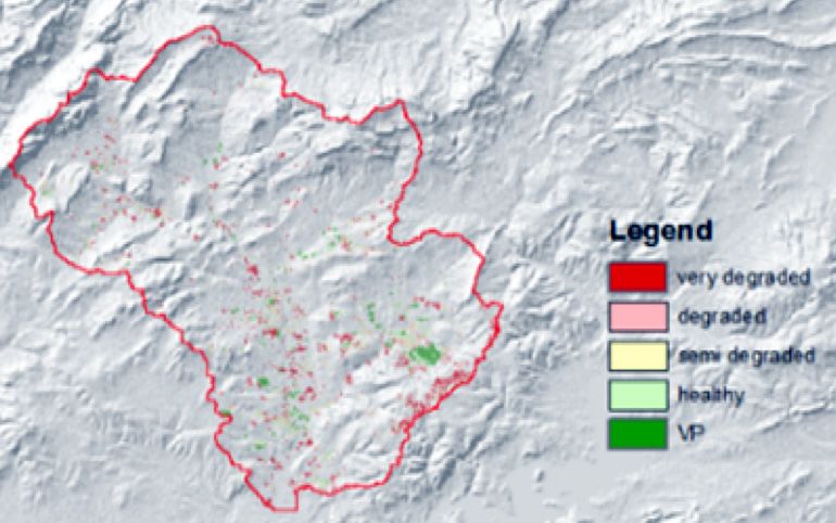
Journal of Mediterranean Ecology vol. 17, 2019

   The Normalized Difference Vegetation Index                   a series of wadis, mainly Wadi Beja (Hidrotehnika-
(NDVI) is widely used to estimate the vegetation                Hidroenergetika 2011).
density and cover. However, the reflectance of veg-                 Most soils are threatened by water erosion, which
etation and thus the NDVI values are influenced by              is provoked by the land topography, 64 % of soils with
several factors such as type of cover, type of land use         a high to steep slope and 36 % of soil with a moderate
and seasonality.                                                slope (AVFA 2016).
                                                                    The lithology of the basin consists mainly of lime-
    In this paper, we propose a simple method to                stone, marl, clay and gypsum (AVFA 2016). Rainfall,
analyze the variance of NDVI signal considering the             characterized by its irregularity, varies from 200 mm
main factors that shape the vegetation. This variance           to 800 mm, depending on the year. The rainfall season
analysis enables us to detect and categorize degrada-           is from winter and autumn, and the period of early
tion in a much more precise way than simple NDVI                spring (AVFA 2016). The maximum temperatures are
analysis. The methodology comprises identifying ho-             recorded at the end of July, when they range between
mogeneous landscape areas in terms of aspect, slope,            38°C and 44°C. Minimum temperatures are recorded at
and land use and disturbance regime (if relevant).              the end of December, when they are between 6°C and
Secondly, the NDVI is calculated from corrected                 8°C (AVFA 2016). 4 different land use classes were
Landsat images and the vegetation potential for each            defined; field crops (75%), grazing lands (10%), for-
landscape is determined based on the percentile (high-          est (5%), permanent crops (7%) and urban area (3%)
est 10% value). Thirdly, the difference between the             which was excluded from the study. Agriculture is the
NDVI value of each pixel and the potential is used              main economic activity and it depends primarily on
to establish degradation categories. Through this               rainfed production systems dominated by cereal crops
methodology, we are able to identify realistic objec-           and small ruminant livestock (Jendoubi et al. 2015).
tives for restoration, allowing a targeted choice of
management options for specific degraded areas. For             2.2. Materials
example, afforestation would only be done in areas                 To create land degradation maps we relied on land
that show potential for Agroforestry. Moreover, we              cover maps derived from DTM and NDVI vegetation
can measure the effectiveness of management prac-               index from Landsat 8 satellite scenes. The Landsat
tices in terms of vegetation growth across different            scenes were selected among all those available in the
landscapes and conditions.                                      green season (out of harvesting) for the year 2015,
    More specifically, three hypotheses derived from            considering only those with less than 20 % of cloud
information provided by experts and stakeholders                cover overall and without clouds on the study site area.
were tested:                                                       Many Landsat and sentinel images downloaded
    (1) Ecosystems are more sensitive to pressure in            from 2013 until 2016 and assessed in order to check
steep and south-facing terrain than in flat and north-          the calendar of the fallow, so we ensure to not to be
facing areas.                                                   confused to consider the no vegetation (fallow) as very
    (2) Present-day inappropriate management remains            degraded lands.
a relevant driver of degradation in steep south terrains.          Detailed information about the data used is pre-
    (3). Third, we aimed to obtain evidence of the im-          sented in table 1.
pact of specific land management practices that had
been identified as promising.
                                                                Table 1. Input data for the creation of land degradation maps.

2. Materials and Method                                          Input data          Wadi Beja watershed
                                                                                     Date : 2009
2.1. Study site                                                  Digital Elevation   Type: Lidar DTM (airborn)
   We selected Wadi Beja watershed in Northwest of               Model               Resolution: 1m resolution
Tunisia, as a representative site that comprise a variety                            Provider: Istituto Geográfico Nacional
of conserved and degraded areas, it has a long history
                                                                                     Path: 192
of field crops land use, and face the risk of monocul-
ture of field crops under inappropriate land manage-                                 Row: 034
                                                                 Landsat scenes
ment practices. This agro-ecological zone covers an                                  Dates: 28-Dec-14, 15-Jan-14, 6-Feb-15, 18-Mar-15,
area of about 33766 ha. The watershed is drained by                                  03-Apr-15, 5-May-15, 6-June-15

                                                            4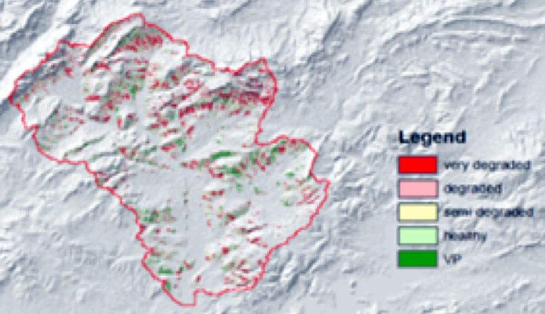
Journal of Mediterranean Ecology vol. 17, 2019

Table 2. Detailed description of visual indicators used for calibration of degradation maps

                                                             Very degraded    Degraded   Semi degraded     Healthy     Vegetation potential
 Indicators                                         Weight
                                                                   (1)           (2)          (3)            (4)               (5)
 Soil fertility (% OC); according to HCN
                                                      3         0-2%          2–4 %           4-6%           6%                >6 %
 analysis results
 Loss of topsoil ; according to the soil map          1        Very high        High       Moderate          low           Insignificant
 Erosion; according to the scoring notation
                                                      2        Very high        High       Moderate          low           Insignificant
 system
 Physical soil deterioration (Structure of soil);
                                                      2        Very high        High       Moderate          low           Insignificant
 Compaction

    In the soil, organic matter is crucial since it holds a                    Field data and observations of degradation, meas-
key position with regard to soil functions (e.g. moisture                  ured through visual indicator were collected to be used
storage capacity, nutrient cycle). Soil organic matter                     to calibrate the degradation maps.
(OM) is also strongly interlinked with various soil deg-                       The land use information served additionally for
radation processes. On the one hand, OM influences the                     the validation of the land degradation maps (table 2).
dynamics of these processes as a crucial force within
the soil (e.g. by determining soil aggregate stability,                        165 field observation points were collected in Wadi
which again is crucial for soil crusting, compaction and                   Beja Watershed (October 2015). To validate and analyze
sheet erosion), and on the other hand, it is affected by                   the results of the degradation maps. All the field data
degradation processes (Heger et al. 2018). The impact                      and observations were clustered into categories from the
on OM content be either direct, through loss of topsoil                    very degraded (1) until vegetation potential (5).
enriched with organic matter as a result of erosion,                           A weight factor was established according to the
or indirect, through reduced vegetation growth and                         expert judgment in order to recognize the importance
subsequently reduced amounts of biomass available                          of the different indicators.
for decomposition and transformation into soil organic                         Furthermore, several informal interviews and
matter (Blaikie 1985; Borelli et al 2016).OM content                       exchanges were organized with land managers, local
may be conserved by adapted land management,                               administrators and land users to obtain information
especially by erosion control, and enriched through                        and discuss the information provided by the degrada-
agronomic and vegetative measures involving cover                          tion maps.
of the soil (e.g. no removal of crop residues or through
permanent vegetative cover) (Lal 2015; Cerdà et al.                        2.3. Methods
2016; Muñoz-Rojas et al. 2015).For this purpose, 165                          For producing the degradation maps data, the fol-
soil samples are collected from the field and processed                    lowing methodology was proposed:
by a combustible CNS analyser, in order to identify
the percentage of organic matter.                                              The landscape units for the analysis of the NDVI
    For the same selected points, a simple template of                     variance are based on land use, slope and aspect cat-
erosion scoring was carried out. The erosion assess-                       egories. As the field crops class represents 75 % from
ment is based on a visual observation that aim to iden-                    the study area, this study focuses more in this famous
tify the type, the state, the density, the stabilization and               land use in order to assess land degradation through
the trend of the assessed erosion. Then a classification                   different conditions. Aspect and slope features were de-
of erosion was carried out.                                                rived from Lidar DTM, aligned and resampled to 30 m.
    Some others soil physical parameters were extracted                    Slope categorization was based on the FAO guidelines
from the available data, such soil map and, soil profiles                  for soil description (Barham et al. 1997). The soil was
and visual observations. The assessment was based on                       grouped in five slope categories. Aspect/Orientation
a predefined set of indicators of soil conditions, along                   was categorized in 2 classes of 180 degrees (north and
with position, topography and land cover information,                      south). Both aspect classifications were tested as input
which they are in direct interaction with the state of                     of the NDVI variance analysis. Details about slope and
the vegetation and seems explicable for the land deg-                      aspect categories are presented in Τable 3.
radation state.

                                                                       5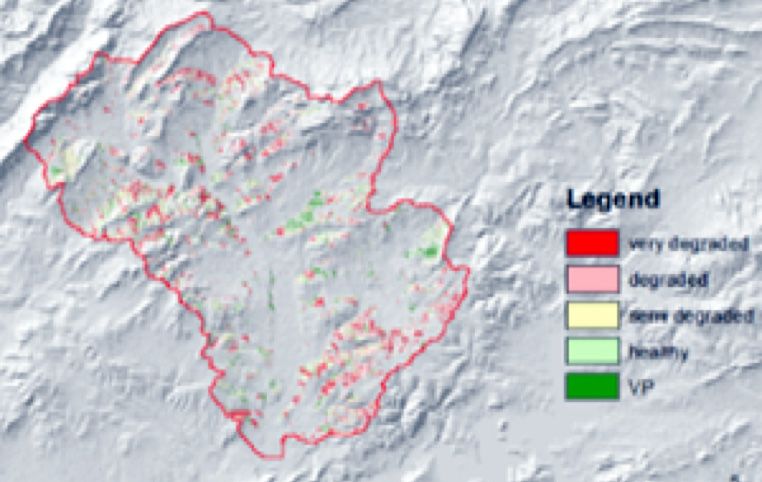
Journal of Mediterranean Ecology vol. 17, 2019

                                                       Figure 1. The overall methodology

Table 3. Aspect and slope categories                                          2009).The landscape unit (LSU) map is obtained by
 Slope                             Aspect classification                      intercepting the raster holding land cover classifica-
                                                                              tion values with those holding slope and aspect values,
 Code    Breaks (in %)             Code     Breaks (in azimuth degrees)
                                                                              followed by a generalization using a window of 3×3
   1     0 to 2 (Flat)               1      0 to 90, 270 to 360 (North)       pixels and the mode value, so that the minimum size
   2     2 to 8 (Moderate)           2      90 to 270 (South)                 of each polygon would be of 9 pixels (8,100 m²).
                                                                                  Secondly, each pixel is classified on a scale of 1
   3     8 to 16 (Sloping)
                                                                              to 5 indicating the degradation level: 1 is the ”very
   4     16 to 30 (Steep)                                                     degraded” and 5 is “potential”, where “potential” in-
   5     30 to 100 (Very Steep)                                               dicates the best situation existing at present for each
                                                                              LSU. We do so by comparing its average NDVI value
                                                                              index value with the distribution of values in the ho-
   Land use maps were elaborated from corrected                               mogeneous landscape unit area, see figure 1.
Landsat 8 Surface Reflectance data and Sentinel.                                  In the majority of studies that investigate NDVI,
Categories have been defined by merging expert’s                              in relation to degradation by evaluating degradation
knowledge on the different land uses and the data                             in time, rather than in space, the mean value or mean
available in the study site.                                                  trend is often considered as reference to identify the
                                                                              positive and negative anomalies. In terms of NDVI
2.3.1. Calculating Vegetation Potential                                       signal, that can highlight the degradation or conser-
   It’s important to assess across landscapes in order                        vation areas (Yengoh et al. 2014) and (Higginbottom
to allow more precise identification of land manage-                          and Symeonakis 2014). Moreover, this is the threshold
ment objectives and restoration options (Bautista et al.                      setting often used “instinctively” by land managers,

                                                                          6
Journal of Mediterranean Ecology vol. 17, 2019

who are able to identify what is degraded based on the                       of what is the potential of that area. Obviously, the
average situation they have experienced. To follow this                      relation between min value, max value and Vegetation
logic, we have adapted the threshold setting used by                         Potential is different in each landscape category.
Ivits et al (2013), using the mean as breakpoint between                         After processing landform units derived from
healthy and degraded areas, and the standard deviation                       DTM, and masked the field crop LSU attribute from
to identify the area of exception deviation from the                         the overall LSU map, a combination between NDVIs
mean, here classified as “potential” (highest NDVI                           maps for each landscape unit was generated, then, a
values) and “very degraded” (lowest NDVI values).                            combination between all the NDVI maps categorized
Once the Vegetation Potential (VP) is identified for                         values (5 categories) was carried out for all the maps
each landscape unit the pixels in the unit are stand-                        (6 times, mean and max).
ardized accordingly on a scale 0-100, where 0 is the
minimum value of the NDVI for that category and 100                          2.3.2 Calibration
is the VP. For interpretation and display, five categories                       The output maps of land cover classification, aspect
are defined: Very degraded, Degraded, Semi-degraded,                         classification and obtained threshold setting for clas-
Healthy and Vegetation Potential.                                            sifying degradation categories were calibrated with
    The process of land degradation can be described                         different parameters and land degradation threshold
as a decline of Net Primary Productivity or a loss of                        settings obtained from the field observations.
fertility (Bai et al. 2008). We classified the pixels based                      The degradation values of the pixel corresponding
on the difference from the areas identified as best, i.e.,                   to each NDVI Mean and Max classification values are
the areas with the highest value of NDVI. At the resolu-                     related with the scale and centered value of all field
tion of Landsat 8 images (30×30 m pixel), the actual                         indicators observations. Correlation between all the
maximum value of NDVI could be misleading, as it                             categories will be assessed in order to deduce map
could correspond to a large tree canopy or to another                        fitness that represent the final degradation maps.
area of very dense vegetation and it shouldn’t be taken                          To gain further information about the impact of
as a reference. Thus, we introduced a buffer on the                          pressure drivers (anthropogenic, climatic and topo-
90th percentile to account for the signal uncertainty                        graphic) on the study site we have analyzed the corre-
and natural variability within the best areas.                               lation between pressure and degradation by aspect and
    Land degradation has to be understood within the                         slope classes in the study site. Our hypothesis was that
local context (Warren, 2002), and is often non-linear                        steeper slopes and south and west exposed areas would
(Scheffer et al. 2009). In this method, 90th percentile                      be more sensitive to pressure, as this factors increase
was set as reference for the potential of vegetation, as                     soil erosion and runoff (slope) and mean temperature
shown in table 4.                                                            and evapotranspiration (aspect), thereby reducing
    Once we have the NDVI values per each landscape                          availability of water and nutrients for the plants.
unit, I calculate the 90th percentile and consider that
the Vegetation Potential (VP). The idea behind it is that
we cannot consider only the max value, as it represents                      3. Results and discussion
too little of the study area and might be misleading.
The best 10% of the pixel appears to give a better idea                      3.1 Results
                                                                                 Unsupervised classification was processed for the
Table 4. LSU map pixel classification according to the threshold
                                                                             corrected Landsat 8 image of June 2015 in order to
setting                                                                      define the major land use classes. The accuracy as-
                                                                             sessment was identified according to the field data,
 Category               Method
                                                                             which is 83%.
                        Absolute value with upper buffer                         At total of 4 major land use classes were found;
 VP                     90th percentile of NDVI value within landscape       field crops (75%), grazing lands (10%), forest (5%),
                        category                                             permanent crops (7%) and urban area (3%) (figure
 Healthy                Between 0.75*VP and VP
                                                                             2). Moreover, as we can see that 75 % of the area is
                                                                             covered by field crops, so we decided to focus in this
 Semi degraded          Between 0.5*VP and 0.75*VP
                                                                             LSU and to extract it from the overall land use map,
 Degraded               Between 0.25*VP and 0.5*VP                           for further assessment. Most of the forest in the study
 Vegetation Potential   Between min value and 0.25*VP                        site are closed and used by military activities, so there
                                                                             is no authorization for access.

                                                                         7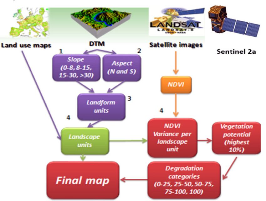
Journal of Mediterranean Ecology vol. 17, 2019

Figure 2. Land use map of Wadi Beja watershed                      Figure 4. Degradation map based on the mean NDVI values

   The degradation maps resulting from the NDVI                    as a degradation map based on NDVI variance across
variance analysis are the combinations of all the NDVI             different landscapes. From this result, we can consider
maps for each landform unit map.                                   the “very degraded and degraded” categories as the
   After checking the maps fitness of all the catego-              hotspots, and the “healthy” category as the bright spots.
rized NDVI values with the categories of field obser-                  We describe the most relevant pattern in the degra-
vation and assessment data, the best correlation was               dation map, based on the information we have collected
observed the values extracted from the mean NDVI                   through other assessment data, stakeholder interactions
map (see figure 3).                                                and field visits.
   There is a linear relationship between the degra-                   We have identified the hot spots (degraded) and
dation classifications derived from the mean NDVI                  the bright spots (healthy) based on our hypothesis and
variance and the mean values per class of the selected             used NDVI as a proxy indicator for land degradation,
indicators. 77 % of correlation was accepted to con-               as suggested by literature and by available data and
sider that the mean NDVI variance can be considered                field observations. We displayed the NDVI variance in

Figure 3. Histograms of the correlation between Maximum and Mean NDVI values with the categories of indicators based on field and
observations data.

                                                               8
Journal of Mediterranean Ecology vol. 17, 2019

South and North in flat slopes and the South and North          to be generally valid in the study site: i.e. “South”
steep slopes as well, to detect the distribution of the         LSUs exhibit a higher distribution NDVI in the very
different categories. Accordingly, the distribution of          degraded category than “North” ones. With regard to
the following NDVI values is indicated from relevant            steepness, the same trend appear to the slopes, which
histograms, see figure 5, 6, 7 and 8.                           we can observe more very degraded areas in the steep
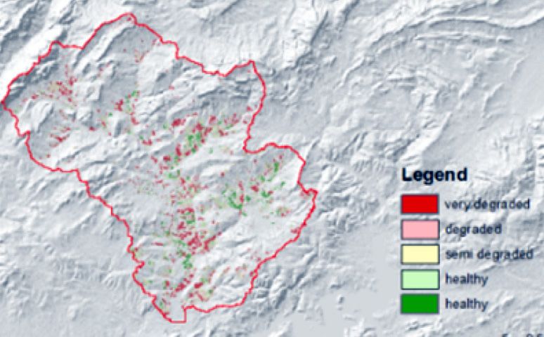
   The figures 5, 6, 7 and 8, show the NDVI variance            slopes terrain. Almost 25 % of the South steep slope
in the different slope and aspects positions, which             is categorized as very degraded areas beside just 13 %
we can get a first impression if we would like to fo-           classified as healthy in the same landform unit. 15 % of
cus for example on the very degraded areas that the             the North steep slopes are classified as very degraded
reddish areas are more appearing in the South steep             beside 19 % of healthy areas. For the north flat face,
map compared to the remaining ones and appearing                20 % of the area is classified as healthy beside 14 %
less in the North flat map. Therefore, we can say that          of very degraded areas.
the hypothesis on the role of the aspect first appears

Figure 5. NDVI variance in South flat slope                     Figure 6. NDVI variance in North flat slope

Figure 7. NDVI variance in South steep slope                    Figure 8. NDVI variance in North steep slope

3.2. Discussions                                                    Not only inappropriate land management lead to
   In order to ensure the identification of hot spots of        “hot spots of soil degradation”. As an example of an
land degradation and bright spots of land conserva-             area showed, stony soils in mountainous regions with
tion, the hot/bright spot map developed for this study          presumably inherently low soil organic carbon SOC
constitutes a simple approach that allows the soil ero-         content may also be classified as hot spots. Thus, in
sion information to be linked with vegetation quality           areas, where also non-loessial soils are present the
indicators in a flexible manner, since it may be used at        classification using the hot/bright spot map will likely
various spatial resolutions and either for raster derived       lead to spurious results.
data (as in this study) or for field data. However, there           A spatially explicit soil type classification is needed,
are also limitations in the explanatory power of the hot/       in order to incorporate effects, which must be attributed
bright spot classification, which need to be addressed          to a specific soil type.
before wider application of the hot/bright spot map is              The assumption with regard to loess soils being
possible:                                                       generally homogeneous (if not affected by degrada-

                                                            9
Journal of Mediterranean Ecology vol. 17, 2019
tion) requires analysis that is more detailed / validation. The result regarding aspects and slopes, appear
Analysis that is more detailed is needed with regard suitable to the hypothesis, it could be related to the
to sites with inherently low SOC. Especially, the re- fact that the south and western exposed LSUs appear
lationship between soil texture and SOC needs to be more sensitive to runoff and water erosion and fur-
analyzed in more detail. ther pressure than others. Land degradation is more
A spatially explicit geology assessment is needed, accelerated in these fragile environments mainly by
in order to incorporate the geologic aspect, which must inappropriate tillage.
be attributed to a specific soil type. Looking at practices to combat desertification, our
We tested the assumption that present day monocul- results stress the perils of widespread conservation ef-
ture was still an important factor in the development forts. Their success rate is low and depends highly on
of the vegetation and the degradation of study site. factors beyond human control, such as slope steepness
This factor was accelerated and recognized by the and aspect, as stressed by other researchers (Príncipe
land management, which inappropriate tillage in steep et al. 2014).
slopes terrain was the main factor, and of course water This can be explained by the higher solar radia-
erosion and runoff. However, some area appears like tion and mean temperatures that are reached during
patches of less vegetation caused from overuse and the afternoon affecting evapotranspiration; moreover,
tillage in the slope direction. humidity is often brought in this area by eastern winds,
In this study case, where erosion consists of three and deposits in eastern exposed LSUs more than west-
phases (uprooting, transport and sedimentation), soil ern exposed.
degradation only involves the destabilization of soil Our assessment of land degradation was based on
structure and macro porosity on the soil. two major steps: (1) identifying LSUs based on land
The degradation of the soil in the present context use system, aspect, and slope; and (2) classifying deg-
resulted essentially from three processes: radation based on the variance of NDVI value within
- The mineralization of organic matter in the soil, each LSU according to a specific threshold setting.
which is more active as the climate is hot and humid; By looking at LSUs we aimed to identify the dif-
- Mineral export by crops, which will lead to a ferences in vegetation development that occur in the
decrease in the activities of micro- fauna and fauna, areas, in order to highlight man-made degradation and
responsible for the macro-porosity of the soil and the other unknown factors that might influence vegetation
diffusion of air and water in the soil; greenness and maintenance. While is it difficult to say
- The skeletonization or enrichment of surface ho- whether the identified degradation patterns are entirely
rizons in sand and gravel by selective erosion of fine related to anthropogenic pressure, the correlation val-
particles, organic matter and nutrients, following the ues between degradation and pressure drivers are a
rainfall. Raindrops fall down to the soil, break up the good indication that the maps indeed describe well the
aggregates, and tear off particles that will form around processes occurring in the study site.
decking and sedimentation crusts that are favorable We interpret the fact that explanation for the NDVI
to runoff. variance in field crops land use system were obtained
Regarding land management, overuse and field when differentiating between different slope and aspect
crops monoculture appears to explain land degradation classes as a confirmation that the resulting degradation
to a relevant degree for north-facing LSUs, while all patterns indeed highlight man made degradation and
other LSUs exhibit low NDVI values. This might be even out differences resulting from aspect and slope.
because low water availability and poor soil fertility The second step in degradation mapping focused
generally limit vegetation growth across all south-, on translating variance in NDVI values into the ap-
east-, or west-facing areas in the site, resulting in a low propriate degradation class. Similar studies have
vegetation cover (and low NDVI values) regardless of showed similar results (Eckert et al. 2015, Liniger et
the land use intensity. al. 2016). There is no agreement among scientists on
Healthy land is primarily located in three areas in how to measure or classify land degradation. Most
the northeast and north-west and center of the study recent methodologies revolve around the use of a set
site. Among the highlighted areas, good land manage- of indicators that vary depending on the specific en-
ment on fairly flat slopes was followed through some vironment considered, and analysis of the causes and
conservation agriculture attempts. Accordingly, they impacts of one or more pressure drivers. This multi-
are less affected by land use and they have been heavily faceted approach is difficult to translate into a logic
maintained by other conservation measures. using a single variable such as NDVI value.
10Journal of Mediterranean Ecology vol. 17, 2019
The specific threshold setting was chosen by cor- them was still important for understanding degradation
relating the degradation classification with the values processes and provided important information to con-
obtained through field observation. This calibration sider when planning land management interventions.
yielded different results for the study site: Threshold Second, some degradation processes do not translate
setting based on the 90th percentile, performed good into a decrease of greenness and can therefore not be
correlation for this site. The mean NDVI values for the detected by means of the NDVI. This was particularly
green season generate the fittest map for land degrada- relevant for example where the main long term impact
tion according to the field data. of – changes in the type of vegetation (e.g. from trees
In the study site, the values of the pixels with the to shrubs) or in the species composition – went unde-
lowest vegetation cover are much more spread out tected in our study. Third, the relation between NDVI
(expressed in the longer tail of the distribution). In and land degradation depends on local soil and climatic
addition to the steep slope position, this may be related characteristics (e.g. 10% of each LSU is considered
to the climatic conditions, which are much drier. Soil as heavily). However, it is possible to try different
characteristics may have an influence as well: In some threshold settings within the same methodology, it is
area, the study case the soil is very shallow, with fre- possible maybe to apply the same methodology and
quent rocks at the surface. By contrast, in some other obtain comparable outputs for ecosystems situated in
areas, soil, is characterized by deep calcific soils that different agro-ecological zones. Besides these intrinsic
are highly prone to erosion. In this case, we have to limitations of the threshold methodology adopted, the
consider that the lowest NDVI values are probably low quality of available land cover maps and of spatial
related to rock outcrops that were recognized as heavily information about land management remains a source
degraded land by the NDVI methodology, while this of uncertainty in the results, and required extra efforts
does not occur in some others areas, where low NDVI to improve the input data using threshold methodolo-
values actually correspond to degraded land also ac- gies (supervised classification, long-term time series
cording to field observations. analysis, Sentinels 2a images, and phenology analysis).
However, the methods selected do take into ac- The resulting land degradation maps proved to be
count the different shapes of the distributions, and are useful exploratory tools for gaining insights into the
thereby applicable on different landscape types within state of field crops ecosystems in the study site, which
the same agro-ecological zone such as in the study of is the strategic and main land use system of the region.
(Liniger et al. 2016). This study aims to investigate how monoculture and
inappropriate tillage influence land degradation, and
to obtain evidence of the impact of land management
4. Conclusion practices. The maps also enabled us to analyze how
The maps obtained by analyzing NDVI variance different landscapes react to pressure and land man-
provided important spatial information on degradation agement, and we can conclude that slope steepness
patterns and conserved areas in a simplified form that increases sensitivity of the land to erosion.,
made it easy to explain to land managers and local Concerning our analysis of the study site, it appears
stakeholders. The map scale was appropriate for in- that monoculture land use is a highly significant driver
vestigating land management in the study sites. Using of degradation, particularly in south – western steep
the information provided by stakeholders, were able slopes terrains, whereas its impact of erosion is more
to identify and explain the overall pattern shown by relevant in the long term. Moreover, there is a signifi-
the map, and to relate this, at least partly, to the mono- cant relationship between topography and land man-
culture risk and water erosion occurrence in the site. agement practices: on steep, south-facing slopes, the
The threshold methodology enabled us to ad- role of erosion is far more important than in flat areas.
equately capture current land degradation, or at least Looking at land management practices, it appears that
those aspects of degradation that translate into reduced successful management in term of restoration is very
vegetation greenness. demanding to achieve, especially on steep, south fac-
Some limits of the methodology emerged when ing slopes. Nonetheless, it appears to have a beneficial
the maps were analyzed in detail. For one thing, local effect, expressed in increased greenness.
microclimatic, topographic (altitude), or soil conditions Using landscape units to translate NDVI values to
influence the location of areas classified as potential. land degradation proved a successful way of highlight-
However, even if these local factors are not related ing the effect of land management and anthropogenic
man-made pressure or land management, highlighting pressure. Further integration of measured data based
11Journal of Mediterranean Ecology vol. 17, 2019
on soil or vegetation parameters, as well as expert dry ecosystems to generate information on degradation
knowledge about the conditions of different LSUs patterns and assess the impact of land management
could allow us to define a universally valid way to practices. Furthermore, the methodology could be
translate NDVI values to land degradation, applicable used for resilience studies and to monitor vegetation
to all ecosystems and agro-climatic zones. Provided recovery after a disturbance across different landscapes
that land use maps and reference points are available, and under different management strategies.
the methodology could easily be implemented in other
5. References Fertility and Vegetation Vigor in Poverty Reduction; The
World Bank: Washington, DC, USA, 2018.
Agence de la Vulgarisation et de la Formation Agricoles Hidrotehnika-Hidroenergetika.2011.Sidi Salem - 1977-
(AVFA) 2016. Agence de la Vulgarisation et de la 1981. http://static.hidrotehnika.rs/en/tunisie/sidi-salem/.
Formation Agricoles. Informations Régionales > Beja. Uskočka 8, Belgrade, Hidrotehnika-Hidroenergetika a.d.
Agricoles. Tunisie, Ministère de l’Agriculture des res- Higginbottom, T.P. and Symeonakis, E. 2014. Assessing land
sources hydrauliques et de la pêche. http://avfa.agrinet. degradation and desertification using vegetation index
tn/fr/informations.php data: Current frameworks and future directions. Remote
Bai, Z.G., Dent, D.L., Olsson, L., Schaepman, M.E. 2008. Sensing6(10): 9552-9575.
Proxy global assessment of land degradation. Soil use Hill, M.J., Braaten, R., Veitch, S.M., Lees B.G. and Sharma
and management 24(3): 223-234. S.,2005. Multi-criteria decision analysis in spatial deci-
Barham, P.,Begg, E., Foote, S., Henderson, J., Jansen, sion support: the ASSESS analytic hierarchy process and
P., Pert, H., Scott, J., Wong, A. and Woolner, D. 1997. the role of quantitative methods and spatially explicit
Guidelines for Guidelines.” Disease Management & analysis. Environmental modelling & software20(7):
Health Outcomes1(4): 197-209. 955-976.
Bautista, S., Aronson J. and Vallejo, V.R. 2009. Land resto- Ivits, E., Cherlet, M., Mehl, W., and Sommer, S. 2013.
ration to combat desertification. Innovative Approaches, Ecosystem functional units characterized by satellite
Quality Control and Project Evaluation. Fundación observed phenology and productivity gradients: A case
CEAM. study for Europe. Ecological indicators27: 17-28.
Blaikie, P. 1985. Political Economy of Soil Erosion in De- Jendoubi, D., Schwilch, G., Liniger, H.P., Hurni, H., Oues-
veloping Countries Longman, London. sar, M. and Hamrouni, H. 2015. Decision-support tools
Borrelli, P., Paustian, K., Panagos, P., Jones, A., Schutt, for assessing land degradation and realising sustainable
B., Lugato, E. 2016. Effect of Good Agricultural and land management in Tunisia. Journal of Mediterranean
Environmental Conditions on erosion and soil organic Ecology
carbon balance: A national case study. Land Use Policy, Lal, R. 2015. Restoring Soil Quality to Mitigate Soil Deg-
50, 408‐421. radation. Sustainability 2015, 7, 5875–5895.
Cerdà, A., González-Pelayo, O., Jordan, A., Pereira, P., No- Liniger, H.P., Jucker Riva, M. and Schwilch, G. 2016.
vara, A., Brevik, E. C., Prosdocimi, M., Mahmoodabadi, Analysis of NDVI variance across landscapes and sea-
M., Shahid, B., Keesstra, S. D., García Orenes, F. and sons allows assessment of degradation and resilience to
Ritsema, C. 2016. The use of barley straw residues to shocks in Mediterranean dry ecosystems. Geophysical
avoid high erosion and runoff rates on persimmon planta- research abstracts, Copernicus Publications.
tions in Eastern Spain under low frequency – high mag- Muñoz-Rojas, A., Jordán, L. M., Zavala, D., De la Rosa,
nitude simulated rainfall events, Soil Res., 54, 54–165, S.K., Abd‐Elmabod, M., Anaya‐Romero 2015. Impact
doi:10.1071/SR15092. of land use and land cover changes on organic carbon
Eckert, S., Hüsler, F., Liniger H.P. and Hodel, E. 2015. Trend stocks in Mediterranean soils (1956–2007). Land De-
analysis of MODIS NDVI time series for detecting land grad. Dev., 26 (2015), pp. 168-179.
degradation and regeneration in Mongolia. Journal of Príncipe, A., Nunes, A., Pinho, P., Do Rosário, L., Correia,
Arid Environments113: 16-28. O. and Branquinho, C.,
Geeson, N.A., Brandt, C.J. and Thornes, J. B. 2003. Medi- 2014. Modeling the long-term natural regeneration potential
terranean desertification: a mosaic of processes and re- of woodlands in semi-arid regions to guide restoration
sponses, John Wiley & Sons. efforts. European journal of forest research133(4): 757.
Heger, M., Zens, G., Bangalor, M. 2018. Does the Environ- Scheffer, M., Bascompte, J., Brock, W.A., Brovkin, V.S.,
ment Matter for Poverty Reduction? The Role of Soil Carpenter, R., Dakos, V., Held, H., Van Nes, E.H., Riet-Journal of Mediterranean Ecology vol. 17, 2019
kerk, M. and Sugihara, G. 2009. Early-warning signals Yengoh, G.T., Dent, D., Olsson, L., Tengberg, A.E. and
for critical transitions. Nature461(7260): 53-59. Tucker, C.J. 2014. The use of the Normalized Difference
Schwilk, D.W., Keeley, J.E., Knapp, E.E., McIver, J., Bailey, Vegetation Index (NDVI) to assess land degradation at
J.D., Fettig, C.J., Fiedler, C.E., Harrod, R.J., Moghad- multiple scales: a review of the current status, future
das, J.J. and Outcalt, K.W. 2009. The national Fire and trends, and practical considerations. Lund University
Fire Surrogate study: effects of fuel reduction methods Center for Sustainability Studies (LUCSUS), and the
on forest vegetation structure and fuels. Ecological Ap- Scientific and Technical Advisory Panel of the Global
plications19(2): 285-304. Environment Facility (STAP/GEF).
Warren, A. 2002. Land degradation is contextual. Land
Degradation & Development13(6): 449-459.
13Journal of Mediterranean Ecology vol. 17, 2019
14You can also read


