Learning Low-dimensional Manifolds for Scoring of Tissue Microarray Images
←
→
Page content transcription
If your browser does not render page correctly, please read the page content below
Learning Low-dimensional Manifolds for
                                          Scoring of Tissue Microarray Images
                                                              Donghui Yan† , Jian Zou$ , Zhenpeng Li‡
                                              †
arXiv:2102.11396v1 [cs.CV] 22 Feb 2021

                                                  Mathematics and Data Science, UMass Dartmouth, MA, USA
                                         $
                                             Mathematical Sciences, Worcester Polytechnic Institute, MA, USA
                                                       ‡
                                                         Statistics, Dali University, Yunnan, China

                                                                           February 24, 2021

                                                                                  Abstract
                                                      Tissue microarray (TMA) images have emerged as an important high-
                                                  throughput tool for cancer study and the validation of biomarkers. Ef-
                                                  forts have been dedicated to further improve the accuracy of TACOMA,
                                                  a cutting-edge automatic scoring algorithm for TMA images. One major
                                                  advance is due to deepTacoma, an algorithm that incorporates suitable
                                                  deep representations of a group nature. Inspired by the recent advance in
                                                  semi-supervised learning and deep learning, we propose mfTacoma to learn
                                                  alternative deep representations in the context of TMA image scoring. In
                                                  particular, mfTacoma learns the low-dimensional manifolds, a common
                                                  latent structure in high dimensional data. Deep representation learning
                                                  and manifold learning typically requires large data. By encoding deep
                                                  representation of the manifolds as regularizing features, mfTacoma effec-
                                                  tively leverages the manifold information that is potentially crude due to
                                                  small data. Our experiments show that deep features by manifolds outper-
                                                  forms two alternatives—deep features by linear manifolds with principal
                                                  component analysis or by leveraging the group property.
                                                      Index terms— Deep representation learning; small data; manifold
                                                  learning; tissue microarray images

                                                  1     Introduction
                                                  Tissue microarray (TMA) images [53, 33, 9] have emerged as an impor-
                                                  tant high-throughput tool for the evaluation of histology-based laboratory
                                                  tests. They are used extensively in cancer studies [20, 9, 25, 50], includ-
                                                  ing clinical outcome analysis [25], tumor progression analysis [38, 1], the
                                                  identification of diagnostic or prognostic factors [19, 1] etc. TMA images
                                                  have also been used in the development and validation of tumor-specific
                                                  biomarkers [25]. Additionally, they are used in imaging genetics [11, 27]
                                                  for the study of genetics alterations. TMA images are produced from thin
                                                  slices of tissue sections cut from small tissue cores (less than 1 mm in
                                                  diameter) which are extracted from tumor blocks. Many slices, typically
                                                  several hundred (possibly from different patients), are arranged as an ar-
                                                  ray and mounted on a TMA slide, and then stained with a tumor-specific

                                                                                      1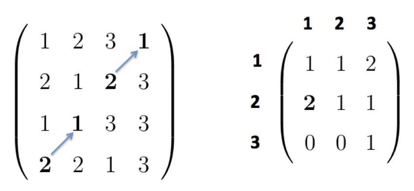
biomarker. A TMA image can be produced for each tissue section (i.e.,
     a cell in the TMA slide) when viewed with a high-resolution microscope.
     Figure 1 is an illustration of the TMA technology.

Figure 1: An illustration of the TMA technology (image courtesy [56]). Small
tissue cores are first extracted from tumor blocks, and stored in archives. Then
thin slices of tissue sections are taken from the tissue core. Hundreds of tissue
sections are mounted, in the form of an array, on a tissue slide, and stained
with tumor-specific biomarkers. A TMA image is captured for each tissue section
when viewed from a high-resolution microscope.

     Spots in a TMA image measure tumor-specific protein expression level.
     The readings of a TMA image are quantified by its staining pattern, which
     is typically summarized as a numerical score by the pathologist. A protein
     marker that is highly expressed in tumor cells will exhibit a qualitatively
     different pattern (e.g., in darker color) from otherwise. Such scores serve
     as a convenient proxy to study the tissue images. To liberate pathologists
     from intensive labors, and also to reduce the inherent variability and sub-
     jectivity with manual scoring [48, 31, 14, 51, 20, 5, 16, 52, 4, 9] of TMA im-
     ages, a number of commercial tools and algorithms have been developed.
     This includes ACIS, Ariol, TMAx and TMALab II for IHC, and AQUA
     [8] for fluorescent images. However, these typically require background
     subtraction, segmentation or landmark selection etc, and are sensitive to
     factors such as IHC staining quality, background antibody binding, hema-
     toxylin counterstaining, and chromogenic reaction products used to detect
     antibody binding [56]. The primary difficulty in TMA image analysis is
     the lack of easily-quantified criteria for scoring—the staining patterns are
     not localized in position, shape or size.

     A major breakthrough was achieved with TACOMA [56], a scoring al-
     gorithm that is comparable to pathologists, in terms of accuracy and re-
     peatability, and is robust against variability in image intensity and stain-
     ing patterns etc. The key insight underlying TACOMA is that, despite sig-
     nificant heterogeneity among TMA images, they exhibit strong statistical
     regularity in the form of visually observable textures or staining patterns.
     Such patterns are captured by a highly effective image statistics—the gray
     level co-occurrence matrix (GLCM). Inspired by the success of deep learn-
     ing [28, 34], deepTacoma [55] incorporates deep representations to meet
     major challenges—heterogeneity and label noise—in the analysis of TMA
     images. The deep features explored by deepTacoma are of a group nature,
     aiming at giving more concrete information than implied by the labels or
     to borrow information from “similar” instances, in analogy to how the
     cluster assumption would help in semi-supervised learning [13, 59].

                                           2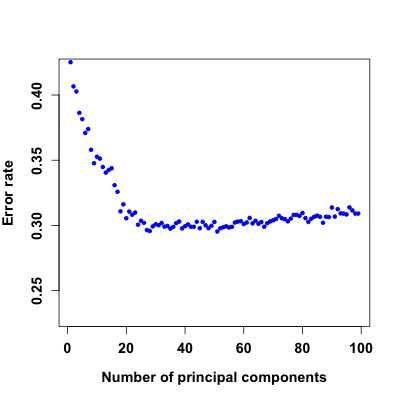
How to further advance the state-of-the-art? Motivated by progress made
with deepTacoma, we will further explore deep representations derived
from latent structures in the data. While deepTacoma makes use of clus-
ters in the data, we pursue the low-dimensional manifolds in the present
work. For high dimensional data, often the data or part of it lie on some
low-dimensional manifolds [47, 43, 17, 26, 12, 6, 41]. Effectively leverag-
ing the manifold information can improve many tasks, such as dimension
reduction or model fitting etc. Indeed, a recent work on the geometry of
deep learning [35] attributes the success of deep learning to the effective-
ness of the deep neural networks in learning such structures in the data.
As our method is built upon TACOMA and uses manifold information,
we term it mfTacoma.

Given the overwhelming popularity of deep learning in image recogni-
tion, it is worthwhile to remark the challenges in applying deep learning
to TMA images [55]. The availability of large training sample, essential
for the success of deep learning, is severely limited for TMA images. TMA
images are much harder to acquire than the usual natural images as they
have to be taken from the human body and captured by high-end micro-
scopes and imaging devices. Their labelling requires substantial expertise
from pathologists. Additionally, the natural and TMA images are of a
different nature in terms of classification. Natural images are typically
formed by a visually sensible image hierarchy, which leads to the neces-
sary sparsity for deep neural networks to succeed [44]. In contrast, the
scoring of TMA images is not about the shape of the staining pattern,
rather the “severity and spread” of staining matters. A further limiting
fact is that TMA images are scored by biomarkers or cancer types; there
are over 100 cancer types according to the US National Cancer Institute
[49].

Our main contributions are as follows. First, we propose an effective ap-
proach to learn the low dimensional manifolds in high dimensional data,
which allows us to advance the state-of-the-art in the scoring of TMA im-
ages. The approach is conceptually simple and easy to implement thanks
to progress in deep neural networks during the last decades. Second, our
approach demonstrates that representing low dimensional manifolds as
regularizing features is a fruitful way of leveraging manifold information,
effectively overcoming the difficulty that shadows many manifold learning
algorithms under small sample. Given the prevalence of low dimensional
manifolds in high dimensional data, our approach may be potentially ap-
plicable to many problems involving high dimensional data.

The remainder of this paper is organized as follows. We describe the
mfTacoma algorithm in Section 2. In Section 3, we present our experi-
mental results. Section 4 provides a summary of the methods and results.
Given the

2     The mfTacoma algorithm
In this section, we will describe the mfTacoma algorithm. The scoring sys-
tems adopted in practice typically use a small number of discrete values,
such as {0, 1, 2, 3}, as the score (or label) for TMA images. The scoring

                                     3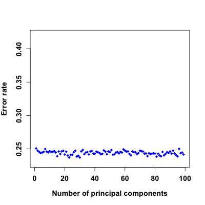
criteria are: ‘0’ indicates a definite negative (no staining of tumor cells),
    ‘3’ a definitive positive (majority cancer cells show dark staining), ‘2’ for
    positive (small portion of tumor cells show staining or a majority show
    weak staining), and ‘1’ indicates weak staining in small part of tumor
    cells, or image in discardable quality [37]. We formulate the scoring of
    TMA images as a classification problem, following ([56]; [55]).

Figure 2: Size of top 100 principal components of TMA images (in GLCM).

    The representations we explore are derived from the low-dimensional man-
    ifold structure in the data. The existence of low-dimensional manifolds in
    high dimensional data is well established [47, 43, 17, 32, 26, 12, 6]. For
    TMA images, as the dimension of the ambient space (i.e., the image size)
    is 1504 x 1440, it is hard to “see” the low-dimensional manifolds. We will
    instead carry out a principal component analysis (PCA) [30, 45, 58, 46]
    on the GLCM of all the TMA images to get a crude sense. Figure 2 shows
    a sharp decay of the principal components and their vanishing beyond the
    50th component, and this clearly implies the existence of low-dimensional
    manifolds. Note that while PCA extracts linear manifolds, the actual
    manifolds maybe be highly nonlinear. Nevertheless, a simple PCA anal-
    ysis should be fairly suggestive of their existence. The low-dimensional
    manifolds are a global property of the data and is beyond what may be
    revealed by features derived from individual data points alone. Therefore
    we expect such information help in the scoring of TMA images. One could
    view the information revealed by manifolds as regularization by problem
    structures in model fitting. Thus a better model (e.g., more stable or
    more accurate) would be expected.

    One technical challenge is how to extract or make use of the manifold
    information from the space formed by the TMA images. Manifold learn-
    ing has been an active research area during the last two decades [32, 12].
    Many work deal with dimension reduction or data visualization, for ex-
    ample, Isomap [47], locally linear embedding [43], Laplacian eigenmaps
    [2], Hessian eigenmaps [17], local tangent space alignment [57], diffusion
    maps [39], metric manifold maps [41]. Some of these were also used as
    a data-driven distance metric for image similarity [42]. A more fruitful

                                         4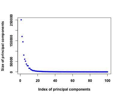
line of work seems to be the use of manifolds for regularization in model
fitting. This is likely due to the difficulty in estimating the manifolds—the
manifolds may be highly nonlinear and the sample size is often dispropor-
tionally small, thus using manifolds as auxiliary information may be more
productive. Indeed Belkin et al [3] successfully used the graph Laplacian
as a regularizer in semi-supervised learning, and Osher and his colleagues
[40] use the dimension of the manifold as a regularizer in image denoising.

We follow a similar line as [3, 40] but with representations derived from the
low-dimensional manifolds as regularizing features to be appended to the
input. This is particularly easy to implement, without having to solve a
complicated optimization problem, and is fairly general. The effectiveness
of using regularizing features has been demonstrated in [55]. Thanks to
the availability and easy implementation of autoencoder [22], we will use
it to extract the low-dimensional manifold representation corresponding
to the TMA images. We term such deep representations as M-features.
Figure 3 is an illustration of the feature hierarchy in mfTacoma.

      Figure 3: Illustration of feature hierarchy in mfTacoma.

The mfTacoma algorithm is fairly simple to describe. First, all TMA
images are converted to their GLCM representations. Then the GLCMs
are input to the autoencoder to extract the deep features, to be con-
catenated with the GLCMs. The manifold-augmented features and their
respective scores are fed to a training algorithm. The trained classifier
will be applied to get scores for TMA images in the test set. To give
an algorithmic description to mfTacoma, assume there are n training in-
stances, m test instances, and N = n + m. Denote the training sample
by (I1 , Y1 ), ..., (In , Yn ) where Ii ’s are images and Yi ’s are scores (thus
Yi ∈ {0, 1, 2, 3}). Let In+1 , ..., In+m be new TMA images that one wish
to score (i.e., the test set has a size of m). mfTacoma is described as
Algorithm 1.

For the rest of this section, we will briefly describe the GLCM and au-
toencoder.

2.1     The gray level co-occurrence matrix
The GLCM is one of the most widely used image statistics for textured
images, such as satellite images and high-resolution tissue images. It

                                       5
Algorithm 1 The mfTacoma algorithm
1: for i = 1 to N
2: Compute GLCM of image Ii ;
3: Denote the resulting GLCM by Xi ;
4: endfor
5: Find manifold representation ∪N N
i=1 {Zi } for ∪i=1 {Xi } with an autoencoder;
M
6: Concatenate Xi and Zi and get Xi , i = 1, ..., N ;
7: Feed ∪n M ˆ
i=1 {(Xi , Yi )} to RF to obtain a classification rule f ;
8: Apply fˆ to Xi to obtain scores for images Ii for i = n + 1, ..., n + m.
M
can be crudely viewed as a “spatial histogram” of neighboring pixels in
an image. It has been successfully applied in a variety of applications
[24, 21, 36, 56, 55]. We follow notations used in [56, 54].
The GLCM is defined with respect to a particular spatial relationship
of two neighboring pixels. The spatial relationship entails two aspects—a
spatial direction, in set {ր, ց, տ, ւ, ↓, ↑, →, ←}, and the
distance between the pair of pixels along the direction. For a given spa-
tial relationship, the GLCM for an image is defined as a Ng × Ng matrix
with its (a, b)-entry being the number of times two pixels with gray val-
ues a, b ∈ {1, 2, ..., Ng } are spatial neighbors; here Ng is the number of
gray levels or quantization levels in the image. Note that, for each spatial
relationship, one can define a GLCM thus one image can correspond to
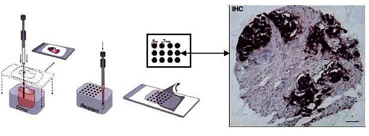
multiple GLCMs. The definition of GLCM is illustrated in Figure 4 with
a toy image (taken from [55]). For a balance of computational efficiency
and discriminative power, we take Ng = 51 and uniform quantization [23]
is applied over the 256 gray levels.
Figure 4: Illustration of GLCM via a toy image (image taken from [55]).
In the 4 × 4 toy image, there are three gray lavels, {1, 2, 3}; the resulting GLCM
for spatial relationship (ր, 1) is a 3 × 3 matrix.
2.2 Autoencoder with deep networks
An autoencoder is a special type of deep neural network with the inputs
and outputs being the same. A neural network is a layered network that
tries to emulate the network of connected biological neurons in the human
brain; it can be used for tasks such as classification or regression. The first
layer of a neural network accepts the input signals, and the last layer for
outputs. Here each node (unit) in the input or output layer corresponding
6to one component of the inputs or outputs when these are treated as a vec-
tor; note for simplicity here we omit the nodes corresponding to the bias
terms. Each node in the intermediate layers (called hidden layers) takes
inputs from all the connecting nodes in the previous layer, then performs
a nonlinear activation operation and outputs the resulting signals to those
connecting nodes in the next layer. As the data flows from one layer to
the next, a weight is applied at all the connecting links. An illustration
of the deep neural network is given in Figure 5. In the following, we will
formally describe the details.
Figure 5: Illustration of deep neural network and autoencoder. X1 , ..., X4 are
components of the inputs and Z1 , Z2 are components of the codewords.
Assume the input data is represented by a matrix XN×p , where N is
the number of data instances and p is the data dimension or the number
of nodes in the input layer. Let the weights to the links connecting the
(i-1)-th and i-th hidden layer be denoted by W (i) , with its dimension de-
termined by the number of nodes involved. Let the output signal from the
i-th hidden layer be denoted by Z (i) . Let σ be the nonlinear activation
function (assume all hidden layers have the same activation function for
simplicity). Assume there are K hidden layers. Then the output signals
at the first hidden layer are given by
Z (1) = σ W (1) X + b(1) .
With the convention Z (0) = X, the output signals at the i-th hidden layer
can be expressed as
Z (i) = σ W (i) Z (i−1) + b(i) , i = 1, 2, ...K.
Often the training of the neural network is formulated as solving
λ
arg min J(W , b, X, Y ) = l Z (K) , Y − · ||W ||, (1)
W ,b 2
where l(.) is a loss function (e.g., squared error for regression or cross
entropy for classification), and ||.|| is a norm such as the L2 norm. The
solution to (1) is often obtained by the back-propagation algorithm. Z (K)
is obtained from X by the composition of a series of functions
σ ◦ W (K) · · · σ ◦ W (2) σ ◦ W (1) ,
7thus it can be written as Z (K) = fW ,b (X) for some function fW ,b , which
can be viewed as a smoothing function (or transformation) of the data.
When the output Y is the same as the input X, the neural network is
called an autoencoder. The deep network in Figure 5 becomes an autoen-
coder when all Xi′ = Xi ; Z1 , Z2 are components of the codewords, that is,
(X1 , ..., X4 ) → (Z1 , Z2 ).
Although not necessary but typically an autoencoder can be divided as
the encoder part and the decoder part which are mirror-symmetric (i.e.,
corresponding layers have the same number of units or connecting weights)
w.r.t. the layer in the center. If some hidden layer has less units than
that of the inputs, that means the data X, at certain stage of its transfor-
mation, has a dimension less than the original dimension thus achieving
a dimension reduction effect. For example, in Figure 5, the original data
dimension is 4 and the transformed data has a dimension of 2. If one is
willing to assume that the activation function is smooth, then the data can
be viewed as lying on a low dimensional manifold. The fitting of the neu-
ral network can thus be viewed as a way of learning the low-dimensional
manifold. As the activation is nonlinear, the resulting manifold is also
nonlinear. As individual hidden layers in a neural network can be viewed
as extracting features of the original data, we will use such features as
representation of the low dimensional manifold. These features are called
M-features, to be appended to the existing GLCM features in the scoring
of TMA images.
Note that we state in Section 1 that for TMA images, the training sample
size is often far less than that required by a typical deep neural network.
However, we could still use the autoencoder, for two reasons. First the
deep representation we will extract with an autoencoder is to be used
for regularization, thus it would be sufficient as long as the representation
captures main features of the manifolds. Second, we can control the size of
the deep network according to the training sample size; indeed we will be
using the simplest autoencoder, that is, with only one hidden layer in this
work. The algorithm for manifolds extraction is simply to extract infor-
mation of the trained hidden layer, when using some deep neural network
package (The deepnet package is used in this work). Let nHidden be the
dimension of the low-dimensional manifold. An algorithmic description is
given as Algorithm 2.
Algorithm 2 mf Learner(X, nHidden)
1: dnn ← dbn.dnn.train(X, X, nHidden);
2: Extract from dnn a low-dimensional representation ∪N
i=1 {Zi };
3: Return(∪Ni=1 {Z i });
3 Experiments
We conduct experiments on TMA images, the data at which our meth-
ods are primarily targeting. The TMA images are taken from the Stan-
ford Tissue Microarray Database (http://tma.stanford.edu/, see [37]).
TMAs corresponding to the biomarker, estrogen receptor (ER), for breast
cancer tissues are used since ER is a known well-studied biomarker. There
8are a total of 695 such TMA images in the database, and each image is
scored at four levels (i.e., label), from {0, 1, 2, 3}.
The GLCM corresponding to (ր, 3) is used, which, according to [56],
is the spatial relationship that leads to the greatest discriminating power
for ER/breast cancer. The pathological interpretation is that, the staining
pattern is approximately rotationally invariant (thus the choice of direc-
tion is no longer important) and ‘3’ is related to the size of the staining
pattern for ER/breast cancer.
For autoencoder, we use the R package deepnet. Random Forests (RF)
[7] is chosen as the classifier due to its superior performance compared to
popular methods such as support vector machines (SVM) [15] and boost-
ing [18], according to large scale simulation studies [10]. This is also true
for the scoring ([56]; [55]) and the segmentation of TMA images [29]. This
is likely due to the high dimensionality (2601 when using GLCM) and the
remarkable feature selection as well as noise-resistance ability of RF, while
SVM and boosting methods are typically prune to those.
For simplicity, the test set error rate is used as our performance met-
ric. In all experiments, a random selection of half of the data are used
for training and the rest for test, and results are averaged over 100 runs.
We conduct two types of experiments. One is to use linear manifolds
extracted by PCA. The other is to use nonlinear manifolds extracted by
autoencoder.
3.1 Experiments with manifolds by PCA
We mention in Section 2 that one can extract linear manifolds with PCA.
How effective are those linear manifolds in the scoring of TMA images?
We distinguish between two cases. One is to use the leading principal
components as sole features to be input the classifier, the other is to use
the leading principal components as regularizing features appended to the
GLCMs. The results are shown in Figure 6 where we produce the test set
error rates when the number of leading principal components increases
up to 100. It can be seen that the PCA features as regularizing features
clearly outperform that using those as sole features with a performance
gap close to about 6%.
3.2 Experiments with manifolds by autoencoder
For nonlinear manifolds with autoencoder, we conduct experiments on
three different cases: 1) Use all the original image pixels as features along
with M-features extracted from the space of the original images; 2) GLCM
features along with M-features extracted from the space of the original im-
ages; 3) GLCM features along with M-features extracted from the space
of GLCMs. We also tried using M-features extracted from the space of
original images alone and that of GLCMs alone, but none gave satisfac-
tory results. Table 1 shows results obtained in the three cases where the
dimension of the low-dimensional manifold varies.
Using original images pixels as features along with manifolds features
extracted from the space of original images does not lead to satisfactory
results, while using GLCMs with manifolds features from the space of
9Figure 6: Test set error rate when including more leading principal components.
Left: using only principal components. Right: using both GLCM features and
principal components.
original images improves marginally over using GLCMs alone. The best
result is achieved at an error rate of 22.85% when using GLCM features
along with M-features extracted from the space of GLCMs with the di-
mension of the manifold being 25. Compared to an error rate of 23.28%
achieved by deepTacoma [55] and 24.79% without using any deep features
by TACOMA [56], the improvement is substantial given that the perfor-
mance by TACOMA [56] already rivals pathologists, and that progress in
this area is typically incremental in nature.
4 Conclusions
Inspired by the recent success of semi-supervised learning and deep learn-
ing, we explore deep representation learning under small data, in the
context of TMA image scoring. In particular, we propose the mfTacoma
algorithm to extract the low-dimensional manifolds in high dimensional
data. Under mfTacoma, deep representations about the manifolds, possi-
bly crude due to small data, are conveniently used as regularizing features
to be appended to the original data features. This turns out to be a simple
and effective way of making use of the low dimensional manifold informa-
tion. Our experiments show that mfTacoma outperforms linear manifold
features extracted by PCA or deep features of a group nature. We con-
sider this a notable improvement over TACOMA and deepTacoma given
that those already rival trained pathologists in the scoring of TMA images
and progress in this area is typically incremental in nature.
Given the prevalence of low dimensional manifolds in high dimensional
data, we expect that deep features derived from low dimensional mani-
folds would help in many applications. Our approach of leveraging the
manifold information as regularizing features will be useful in small data
setting, where one may incorporate feature weights by accounting for the
sample size or data quality.
10Features Dim. of manifold Error rate
GLCM — 24.79%
Image + AE image features 100 29.89%
50 29.88%
25 29.90%
GLCM + AE image features 400 24.51%
300 24.64%
200 24.03%
100 24.63%
50 24.42%
25 24.36%
10 24.59%
GLCM + AE GLCM features 200 24.72%
100 24.66%
50 24.59%
40 23.84%
30 23.23%
25 22.85%
20 23.08%
10 23.75%
Table 1: Error rate in scoring TMA images when using different deep features
under different manifold dimensions. Note that the first row corresponds to re-
sults obtained by RF on the GLCM features alone (i.e., without deep features).
Here ‘Image’ indicates when the original image pixels are used as features, ‘AE
image features’ indicates manifold features extracted from the space of the orig-
inal TMA images, ‘AE GLCM features’ indicates manifold features extracted
from the space of the GLCM of the TMA images.
References
[1] A. Beck, A. Sangoi, S. Leung, R. Marinelli, T. Nielsen TO, M. van de
Vijver, R. West, M. van de Rijn, and D. Koller. Systematic analysis of
breast cancer morphology uncovers stromal features associated with
survival. Science Translational Medicine, 3(108):108–113, 2011.
[2] M. Belkin and P. Niyogi. Laplacian eigenmaps for dimensionality
reduction and data representation. Neural Computation, 15:1373–
1396, 2003.
[3] M. Belkin, P. Niyogi, and V. Sindhwani. Manifold regularization: A
geometric framework for learning from labeled and unlabeled exam-
ples. Journal of Machine Learning Research, 7:2399–2434, 2006.
[4] S. Bentzen, F. Buffa, and G. Wilson. Multiple biomarker tissue
microarrays: bioinformatics and practical approaches. Cancer and
Metastasis Reviews, 27(3):481–494, 2008.
[5] A. Berger, D. Davis, C. Tellez, V. Prieto, J. Gershenwald, M. John-
son, D. Rimm, and M. Bar-Eli. Automated quantitative analysis
of activator protein-2 α subcellular expression in melanoma tissue
microarrays correlates with survival prediction. Cancer research,
65(23):11185, 2005.
11[6] P. J. Bickel and D. Yan. Sparsity and the possibility of inference.
Sankhya: The Indian Journal of Statistics, Series A (2008-), 70(1):1–
24, 2008.
[7] L. Breiman. Random Forests. Machine Learning, 45(1):5–32, 2001.
[8] R. Camp, G. Chung, D. Rimm, et al. Automated subcellular local-
ization and quantification of protein expression in tissue microarrays.
Nature medicine, 8(11):1323–1327, 2002.
[9] R. Camp, V. Neumeister, and D. Rimm. A decade of tissue microar-
rays: progress in the discovery and validation of cancer biomarkers.
Journal of Clinical Oncology, 26(34):5630–5637, 2008.
[10] R. Caruana, N. Karampatziakis, and A. Yessenalina. An empirical
evaluation of supervised learning in high dimensions. In Proceedings
of the Twenty-Fifth International Conference on Machine Learning
(ICML), pages 96–103, 2008.
[11] B. J. Casey, F. Soliman, K. G. Bath, and C. E. Glatt. Imaging
genetics and development: challenges and promises. Human Brain
Mapping, 31(6):838–851, 2010.
[12] L. Cayton. Algorithms for manifold learning. Technical Report
CS2008-0923, Department of Computer Science, UC San Diego,
2008.
[13] O. Chapelle, J. Weston, and B. Schölkopf. Cluster kernels for semi-
supervised learning. In Advances in Neural Information Processing
Systems 15, pages 601–608, 2003.
[14] G. Chung, E. Kielhorn, and D. Rimm. Subjective differences in out-
come are seen as a function of the immunohistochemical method used
on a colorectal cancer tissue microarray. Clinical Colorectal Cancer,
1(4):237–242, 2002.
[15] C. Cortes and V. N. Vapnik. Support-vector networks. Machine
Learning, 20(3):273–297, 1995.
[16] K. DiVito and R. Camp. Tissue microarrays–automated analysis and
future directions. Breast Cancer Online, 8(7), 2005.
[17] D. Donoho and C. Grimes. Hessian eigenmaps: Locally linear em-
bedding techniques for high-dimensional data. Proceedings of the
National Academy of Sciences, U. S. A., 100(10):5591–5596, 2003.
[18] Y. Freund and R. Schapire. Experiments with a new boosting algo-
rithm. In International Conference on Machine Learning (ICML),
1996.
[19] G. Fromont, M. Roupret, N. Amira, M. Sibony, G. Vallancien, P. Va-
lidire, and O. Cussenot. Tissue microarray analysis of the prognostic
value of E-Cadherin, Ki67, p53, p27, Survivin and MSH2 expression
in upper urinary tract transitional cell Carcinoma. European Urology,
48(5):764–770, 2005.
[20] J. Giltnane and D. Rimm. Technology insight: identification of
biomarkers with tissue microarray technology. Nature Clinical Prac-
tice Oncology, 1(2):104–111, 2004.
[21] P. Gong, D. Marceau, and P. J. Howarth. A comparison of spatial
feature extraction algorithms for land-use classification with SPOT
HRV data. Remote Sensing of Environment, 40:137–151, 1992.
12[22] I. Goodfellow, Y. Bengio, and A. Courville. Deep Learning. The MIT
Press, 2016.
[23] R. M. Gray and D. L. Neuhoff. Quantization. IEEE Transactions of
Information Theory, 44(6):2325–2383, 1998.
[24] R. M. Haralick. Statistical and structural approaches to texture.
Proceedings of IEEE, 67(5):786–803, 1979.
[25] S. Hassan, C. Ferrario, A. Mamo, and M. Basik. Tissue microar-
rays: emerging standard for biomarker validation. Current Opinion
in Biotechnology, 19(1):19–25, 2008.
[26] C. Hegde, M. Wakin, and R. Baraniuk. Random projections for
manifold learning. In Neural Information Processing Systems (NIPS),
volume 20, 2007.
[27] D. Hibar, O. Kohannim, J. Stein, M.-C. Chiang, and P. Thompson.
Multilocus genetic analysis of brain images. Frontiers in Genetics,
2(73):1–11, 2011.
[28] G. Hinton and R. Salakhutdinov. Reducing the dimensionality of
data with neural networks. Science, 313:504–507, 2006.
[29] S. Holmes, A. Kapelner, and P. Lee. An interactive Java statistical
image segmentation system: Gemident. Journal of Statistical Soft-
ware, 30(10):1–20, 2009.
[30] H. Hotelling. Analysis of a complex of statistical variables into prin-
cipal components. Journal of Educational Psychology, 24:417–441,
1933.
[31] C. Hsu, D. Ho, C. Yang, C. Lai, I. Yu, and H. Chiang. Interobserver
reproducibility of Her-2/neu protein overexpression in invasive breast
carcinoma using the DAKO HercepTest. American journal of clinical
pathology, 118(5):693–698, 2002.
[32] X. Huo, X. Ni, and A. Smith. A survey of manifold-based learning
methods. Recent Advances in Data Mining of Enterprise Data, pages
691–745, 2007.
[33] J. Kononen, L. Bubendorf, A. Kallionimeni, M. Bärlund, P. Schraml,
S. Leighton, J. Torhorst, M. Mihatsch, G. Sauter, and O. Kallioni-
meni. Tissue microarrays for high-throughput molecular profiling of
tumor specimens. Nature Medicine, 4(7):844–847, 1998.
[34] Y. LeCun, Y. Bengio, and G. Hinton. Deep learning. Nature,
521:436–444, 2015.
[35] N. Lei, Z. Luo, S.-T. Yau, and D. X. Gu. Geometric understanding
of deep learning. arXiv:1805.10451, 2018.
[36] C. D. Lloyd, S. Berberoglu, P. J. Curran, and P. M. Atkinson.
A comparison of texture measures for the per-field classification of
Mediterranean land cover. International Journal of Remote Sensing,
25(19):3943–3965, 2004.
[37] R. Marinelli, K. Montgomery, C. Liu, N. Shah, W. Prapong,
M. Nitzberg, Z. Zachariah, G. Sherlock, Y. Natkunam, R. West,
et al. The Stanford tissue microarray database. Nucleic Acids Re-
search, 36:D871–877, 2007.
[38] S. Mousses, L. Bubendorf, U. Wagner, G. Hostetter, J. Kononen,
R. Cornelison, N. Goldberger, A. Elkahloun, N. Willi, P. Koivisto,
13W. Ferhle, M. Raffeld, G. Sauter, and O. Kallioniemi. Clinical valida-
tion of candidate genes associated with prostate cancer progression in
the cwr22 model system using tissue microarrays. Cancer Research,
62(5):1256–1260, 2002.
[39] B. Nadler, S. Lafon, R. Coifman, and I. G. Kevrekidis. Diffusion
maps - a probabilistic interpretation for spectral embedding and clus-
tering algorithms. Principal Manifolds for Data Visualization and
Dimension Reduction (Lecture Notes in Computational Science and
Engineering), 58:238–260, 2007.
[40] S. Osher, Z. Shi, and W. Zhu. Low dimensional manifold model for
image processing. SIAM Journal on Imaging Sciences, 10(4):1669–
1690, 2017.
[41] D. Perraul-Joncas and M. Meila. Non-linear dimensionality reduc-
tion: Riemannian metric estimation and the problem of geometric
discovery. arXiv:1305.7255, 2013.
[42] R. Pless and R. Souvenir. A survey of manifold learning for images.
IPSJ Transactions on Computer Vision and Applications, pages 83–
94, 2009.
[43] S. Roweis and L. Saul. Nonlinear dimensionality reduction by locally
linear embedding. Science, 290(5500):2323–2326, 2000.
[44] J. Schmidt-Hieber. Nonparametric regression using deep neural net-
works with ReLU activation function. arXiv:1708.06633, 2017.
[45] C. Shahabi and D. Yan. Real-time pattern isolation and recognition
over immersive sensor data streams. In Proceedings of the 9th Inter-
national conference on multi-media modeling, pages 93–113, 2003.
[46] J. Shlens. A tutorial on principal component analysis.
arXiv:1404.1100, 2014.
[47] J. B. Tenenbaum, V. de Silva, and J. C. Langford. A global geo-
metric framework for nonlinear dimensionality reduction. Science,
290(5500):2319–2323, 2000.
[48] T. Thomson, M. Hayes, J. Spinelli, E. Hilland, C. Sawrenko,
D. Phillips, B. Dupuis, and R. Parker. HER-2/neu in breast cancer:
interobserver variability and performance of immunohistochemistry
with 4 antibodies compared with fluorescent in situ hybridization.
Modern Pathology, 14(11):1079–1086, 2001.
[49] US National Cancer Institute. https://www.cancer.gov/about-cancer/understanding/what-is-cancer.
[50] D. Voduc, C. Kenney, and T. Nielsen. Tissue microarrays in clinical
oncology. Seminars in radiation oncology, 18(2):89–97, 2008.
[51] H. Vrolijk, W. Sloos, W. Mesker, P. Franken, R. Fodde, H. Morreau,
and H. Tanke. Automated Acquisition of Stained Tissue Microarrays
for High-Throughput Evaluation of Molecular Targets. Journal of
Molecular Diagnostics, 5(3):160–167, 2003.
[52] R. Walker. Quantification of immunohistochemistry - issues concern-
ing methods, utility and semiquantitative assessment I. Histopathol-
ogy, 49(4):406–410, 2006.
[53] W. H. Wan, M. B. Fortuna, and P. Furmanski. A rapid and efficient
method for testing immunohistochemical reactivity of monoclonal
antibodies against multiple tissue samples simultaneously. Journal
of Immunological Methods, 103:121–129, 1987.
14[54] D. Yan, P. Bickel, and P. Gong. A bottom-up approach for texture
modeling with application to Ikonos image classification. Submitted,
2018.
[55] D. Yan, T. W. Randolph, J. Zou, and P. Gong. Incorporating deep
features in the analysis of tissue microarray images. Statistics and
Its Interface, 12(2):283–293, 2019.
[56] D. Yan, P. Wang, B. S. Knudsen, M. Linden, and T. W. Randolph.
Statistical methods for tissue microarray images–algorithmic scoring
and co-training. The Annals of Applied Statistics, 6(3):1280–1305,
2012.
[57] Z. Zhang and H. Zha. Principal manifolds and nonlinear dimension
reduction via local tangent space alignment. SIAM Journal on Sci-
entific Computing, 26(1):313–338, 2004.
[58] H. Zhao, P. C. Yuen, and J. T. Kwok. A novel incremental principal
component analysis and its application for face recognition. IEEE
Transactions on Systems, Man, and Cybernetics–Part B: Cybernet-
ics, 36(4):873–886, 2006.
[59] X. Zhu. Semi-supervised learning literature survey. TR 1530, Depart-
ment of Computer Science, University of Wisconsin-Madison, 2008.
15You can also read