Learning on the Edge: Explicit Boundary Handling in CNNs - BMVC 2018
←
→
Page content transcription
If your browser does not render page correctly, please read the page content below
INNAMORATI ET AL.: LEARNING ON THE EDGE                                                                 1

Learning on the Edge:
Explicit Boundary Handling in CNNs
Carlo Innamorati                                            University College London
c.innamorati@cs.ucl.ac.uk
Tobias Ritschel
t.ritschel@cs.ucl.ac.uk
Tim Weyrich
t.weyrich@cs.ucl.ac.uk
Niloy J. Mitra
n.mitra@cs.ucl.ac.uk

                                                     Abstract
            Convolutional neural networks (CNNs) handle the case where filters extend beyond the
       image boundary using several heuristics, such as zero, repeat or mean padding. These
       schemes are applied in an ad-hoc fashion and, being weakly related to the image content
       and oblivious of the target task, result in low output quality at the boundary. In this paper,
       we propose a simple and effective improvement that learns the boundary handling itself.
       At training-time, the network is provided with a separate set of explicit boundary
       filters. At testing-time, we use these filters which have learned to extrapolate features at
       the boundary in an optimal way for the specific task. Our extensive evaluation, over a
       wide range of architectural changes (variations of layers, feature channels, or both), shows
       how the explicit filters result in improved boundary handling. Consequently, we
       demonstrate an improvement of 5 % to 20 % across the board of typical CNN applications
       (colorization, de-Bayering, optical flow, and disparity estimation).

1     Introduction
When performing convolutions on a finite domain, boundary rules are required as the ker-
nel’s support extends beyond the edge. For convolutional neural networks (CNNs), many
discrete filter kernels “slide” over a 2D image and typically boundary rules including zero,
reflect, mean, clamp are used to extrapolate values outside the image.
    Considering a simple detection filter (Fig. 1a) applied to a diagonal feature (Fig. 1b), we
see that no boundary rule is ever ideal: zero will create a black boundary halo (Fig. 1c), using
the mean color will reduce but not remove the issue (Fig. 1d), reflect and clamp (Fig. 1e
and 1f) will create different kinks in a diagonal edge where the ground-truth continuation
would be straight. In Fig. 1 we visualize this as the error between the ideal response and the
response we would observe at a location if a feature was present. In practical feature channels,
these will manifest as false positive and negative images. These deteriorate overall feature
quality, not only on the boundary but also inside. Another, equally unsatisfying, solution is
to execute the CNN only on a “valid” interior part of the input image (crop), or to execute it
 c 2018. The copyright of this document resides with its authors.
It may be distributed unchanged freely in print or electronic forms.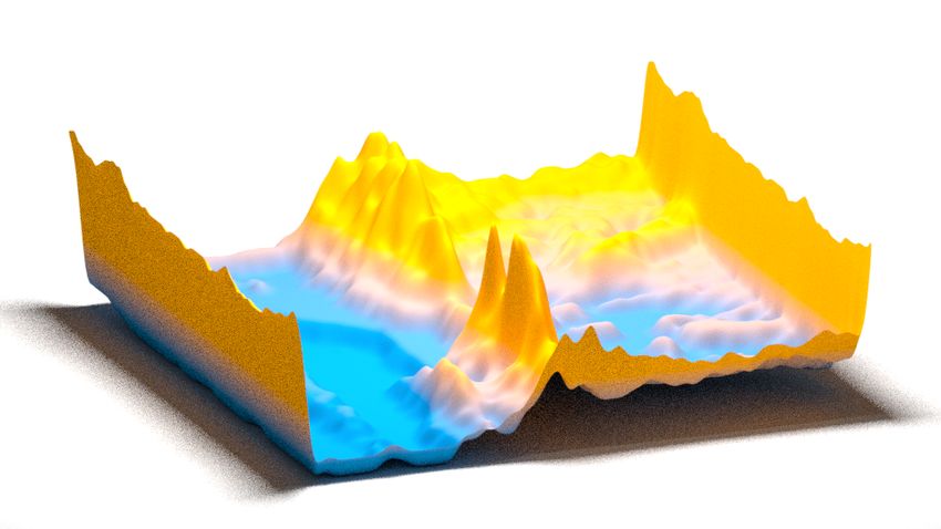
2                                                                INNAMORATI ET AL.: LEARNING ON THE EDGE
a)            b)                        c)                     d)                     e)                        f)
              natural

                                                                                      reflect

                                                                                                                clamp
                                        zero

                                                               mean
     Filter
                        Image   Error          Image   Error          Image   Error             Image   Error           Image   Error
                        World                  World                  World                     World                   World

Figure 1: Applying a feature detection-like filter (a) to an image with different boundary
rules (b–f). We show the error as the ratio of the ideal and the observed response. A bright
value means a low error due to a ratio of 1 i. e., the response is similar to the ideal condition.
Darker values indicate a deterioration.

multiple times and merge the outcome slide. Working in lower or multiple resolutions, the
problem is even stronger, as low-resolution images have a higher percentage of boundary
pixels. In a typical modern encoder-decoder [11], all will eventually become boundary pixels
at some step.

    Having a second thought on what a 2D image actually is, we see, that the ideal boundary
rule would be the one that extends the content exactly to the values an image taken with a
larger sensor would have contained. Such a rule appears elusively hard to come by as it relies
on information not observed. We cannot decide with certainty from observing the yellow part
inside the image in Fig. 1b how the part outside the image continues – what if the yellow
structure really stopped? – and therefore it is unknown what the filter response should be.
However, neural networks have the ability to extrapolate information from a context, for
example in in-painting tasks [10]. Here, this context is the image part inside the boundary.
Given this observation, not every extension is equally likely. Most human observers would
follow the Gestalt assumption of continuity and predict the yellow bar to continue at constant
slope outside the image. Can a CNN do this extrapolation while extracting features?

    Addressing the boundary challenge, and making use of a CNN’s extrapolating power, we
propose the use of a novel explicit boundary rule in CNNs. As such rules will have to
depend on the image content and the spatial location of that content, we advocate to model
them as a set of learned boundary filters that simply replace the non-boundary filters when
executed on the boundary. These boundary filters are supposed to produce exactly the same
feature channels the non-boundary filters produce. Every boundary configuration (upper
edge, lower left corner, etc.) has a different filter. This implies, that they incur no time or
space overhead at runtime. At training-time, boundary and non-boundary filters are jointly
optimized and no additional steps are required.

    It seems, that introducing more degrees of freedom increases the optimization challenge.
However, introducing the right degrees of freedom, can actually turn an unsolvable problem
into separate tasks that have simple independent solutions, as we conclude from a reduction
of error both at the interior and at the edges, when using our method.

    After reviewing previous work and introducing our formalism, we demonstrate how using
explicit boundary conditions can improve the quality across a wide range of possible
architectures (Sec. 4). We next show improvement in performance for tasks such as de-noising
and de-bayering [7], colorization [15] as well as disparity and scene flow [5], in Sec. 5.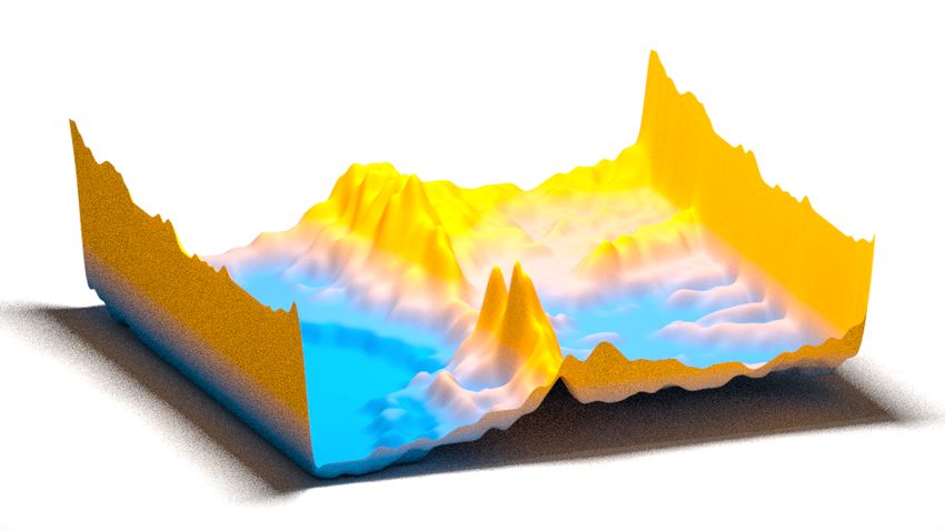
INNAMORATI ET AL.: LEARNING ON THE EDGE                                                          3

2    Previous Work
Our work extends deep convolutional neural networks [8] (CNNs). To our knowledge, the
immediate effect of boundary handling has not been looked into explicitly. CNNs owe a part
of their effectiveness to weight-sharing or shift-invariance property: only a single convolution
needs to be optimized that is applied to the entire image [6]. Doing so, inevitably, the filter
kernel will touch upon the image boundary at some point. Classic CNNs use zero padding
[2], i. e., they enlarge the image by the filter kernel size they use, or directly crop, i. e., run
only on a subset [9] and discard the boundary. Another simple solution is to perform filtering
with an arbitrary boundary handling and crop the part of the image that remains unaffected: if
the filter is centered and 3 pixels wide, a 100×100 pixel image is cropped to 98×98 pixels.
This works in a single resolution, but multiple layers, in particular at multiple resolutions,
grow the region affected by the boundary linearly or even exponentially. For example, the
seminal U-net [11] employs a complicated sliding scheme to produce central patches from a
context that is affected by the boundary, effectively computing a large fraction of values that
are never used. We show how exactly such a U-net-like architecture can be combined with
explicit boundaries to realize a better efficacy with lower implementation and runtime
overhead. Other work has extended the notion of invariance to flips [3] and rotations [14].
Our extension could be seen as adding invariance under boundary conditions. For some
tasks like in-panting, however, invariance is not desired, and translation-variant convolutions
are used [10]. This paper shares the idea to use different convolutions in different spatial
locations. Uhrig et al. have weighted convolutions to skip pixels undefined at test time [13].
In our setting, the undefined pixels are known at train time to always fall on the boundary. By
making this explicit to the learning, it can capitalize on knowing how the image extends.

3    Explicit Boundary Rules
In this section we will define convolutions that can account for explicit boundary rules,
before discussing the loss and implementation options.

Convolution Key to explicit boundary handling is a domain decomposition. Intuitively,
in our approach, instead of running the same filter for every pixel, different filters are run at
the boundary. In any case, they compute the same feature. This is done independently for
every convolution kernel in the network. For simplicity, we will here explain the idea for
a single kernel that computes a single feature. The extension to many kernels and features
is straightforward. Again, for simplicity, we describe the procedure for a 2D convolution,
mapping scalar input to scalar output. The 3D convolution, mapping higher-dimensional input
to scalar output is derived similarly.
    A common zero boundary handling convolution ∗0 of an input image f (in) with the
kernel g is defined as
                                          (
                       (out)                f (in) [x + y] · g[y] if x + y ∈ D
                     f       [x] ∗0 g = ∑                                                     (1)
                                       y∈K 0                      otherwise,

where K is the kernel domain, such as {−1, 0, 1}2 and D is the image domain in pixel
coordinates from zero to image width and height, respectively. We extend this to explicit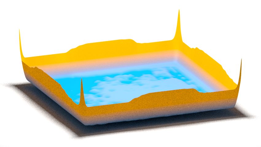
4                                                 INNAMORATI ET AL.: LEARNING ON THE EDGE

                                   g1        g2        g3       g4   g5        g6       g7        g8       g9
       Edge
                                   =               +        +        +    +         +             +    +        +
      Corner

      Interior                     f (out)

 g1           g2       g3         g4              g5            g6        g7                 g8            g9

Figure 2: Example domain decomposition for a 5×5 image. Colors encode different filters.

boundary handling ∗e using a family of kernels g1,...n as
                                           (
                 (out)                       f (in) [x + y] · gs[x] [y] if x + y ∈ D
               f       [x] ∗e g1,...,n = ∑                                                                          (2)
                                        y∈K 0                           otherwise,

where s[x] is a selection function that returns the index from 1 to n of the filter to be used at
position x (Fig. 2). The number of filters n depends on the size of the receptive field: For a
3×3 filter it is 9 cases, for larger fields it is more.

Loss The loss is defined on multiple filter kernel values g1,...n instead of a single kernel. As
this construction comprises of linear operations only (the selection function can be written as
nine multiplications of nine convolution results with nine masks that are 0 or 1 and a final
addition), it is back-propagatable.

Implementation A few things are worth noting for the implementation. First, applying
multiple kernels in this fashion has the same complexity as applying a single kernel. Con-
volution in the Fourier domain, where costs would differ, is typically not done for kernels
of this size. Second, the memory requirement is the same as when running with common
boundary conditions. All kernels jointly output one single feature image. The boundary filters
are never run and no result is stored at the interior. The only overhead is in storing the filter
masks. In practice however, implementation constants might differ between implementations,
in particular for parallel machines (GPUs).
    The first practical option for implementation is the most compatible one that just performs
all nine convolutions on the entire image and later composes the nine images into a single
image. This indeed has compute and memory cost linear in the number of filters, i. e., nine
times more expensive, both for training and deployment
    To avoid the overhead, without having to access the low level code of the framework in
use, the additional kernels can be trained on the specific sub-parts of the input that they act on
and then composited back to form the output.

4     Analysis
We will now analyze the effect of border handling for a simplified task and different networks:
learning how to perform a Gaussian blur of a fixed size. Despite the apparent simplicity,
we will see, how many different variants of a state-of-the-art U-net-like [11] architecture all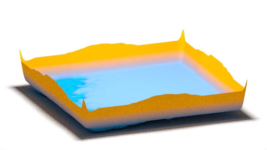
INNAMORATI ET AL.: LEARNING ON THE EDGE                                                         5

suffer from similar boundary handling problems. This indicates, that the deteriorating effect
of unsuccessful boundary handling cannot be overcome by adapting the network structure,
but needs the fundamentally different domain decomposition we suggest.

4.1    Methods
Task The tasks is to learn the effect of a Gauss filter of size 13×13 to 128×128 images,
obtained from the dataset used for the ILSVRC [12] competition, comprising of over one
million images selected from ImageNet [4]. The ground truths were computed over 128 +
12 × 128 + 12 images, which were then cropped to 128×128.

Metrics We compare to the reference by means of the MSE metric, which was also used as
the loss function. The models were selected by comparing the loss values over validation set,
while the reported loss values were separately computed over a test set comprising of 10 k
examples.

Architecture We use a family of architectures to cover both breadth and width of the
network. The breadth is controlled by the number of feature channels and the depth by the
number of layers. More specifically, the architecture comprises of nl layers. Each layer
performs a convolution to produce nf feature channels, followed by a ReLU non-linearity.
We choose such an architecture, to show that the effect of boundary issues is not limited to a
special setting but remains fundamental.

Boundary handling We include our explicit handling, as well as the classic zero
strategy that assumes the image to be 0 outside the domain and reflect padding, that
reflects the image coordinate around the edge or corner.

4.2    Experiments
Here, we study how different architecture parameters affect boundary quality for each type of
boundary handling.

Varying depth When varying depth nl from a single up to 7 layers (Fig. 3a) we find, that our
explicit boundary handling performs best on all levels, followed by reflect boundary
handling and zero. The feature channel count is held fixed at nf = 3.

Varying feature count When varying feature channel count nf , it can be seen that explicit
leads the board, followed by reflect and zero (Fig. 3b). The depth is held fixed at nd = 2.

Varying feature count and depth When varying both depth nl and feature channel count
nf , seen in Fig. 3, c we find, that again no architectural choice can compensate for the boundary
effects. Each of the seven steps increase feature count by 3 and depth by 1.

Statistical analysis A two-sided t test (N = 10, 000) rejects the hypothesis that our method
is the same as any other method for any task with p < .001.
6                                                                           INNAMORATI ET AL.: LEARNING ON THE EDGE

           1         a)                  zero
                                                             1         b)                                   1          c)

                                                                                                                                      Reference
                                                                                      Input
                                         reflect
                                         explicit
         Error

                                                           Error

                                                                                                         Error
           0                                                0                                              0
                 1      2    3   4    5   6       7                1    2   3     4   5       6   7              1/3   2/6   3/9 4/12 5/15 6/18 7/21
                            Feature count                                       Depth                                  Depth + Feature count
                 zero          reflect          explicit         zero           reflect       explicit       zero             reflect             explicit
Result
Error

Figure 3: Analysis of different architectural choices using different boundary handling (colors).
First, (a) we increase feature channel count (first plot and columns of insets). The vertical
axis shows log error for the MSE (our loss) and the horizontal axis different operational
points. Second (b), depth of the network is increased (second plot and first 4 columns of
insets). Third, (c) both are increased jointly. The second row of insets shows the best (most
similar to a reference) result for each boundary method (column) across the variation of one
architectural parameter for a random image patch (input an reference result seen in corner).

5                 Applications
Now, we compare different boundary handling methods in several typical applications.

5.1                  Methods
Architecture We use an encoder-decoder network with skip connections [11] optimized for
the MSE loss using the ADAM optimizer . Details are shown in our supplemental materials.
The architecture is different from the simplified one in the previous section where it was
important to systematically explore many possible variants. The encoding proceeds in 3 × 3
convolution steps 1 to 7, increasing the number of feature channels from 1 to 256. There is
a flat 1×1 convolution at the most abstract representation at stage 8. Decoding happens on
stages 9 to 14. This step resizes the image, convolves with stride 1 and outputs the stated
number of feature, followed by a concatenate convolution by the stated skip ID and finally a
convolution with stride 1 that outputs the stated number of features (ResConv).
     Note, that boundary handling is required at all stages except 8. For the down-branch 1–7
this can be less relevant as strides do not produce all edge cases we handle, e. g., the boundary
pixels on the bottom of the input are skipped in an even resolution scheme.

Measure We apply different task-specific measures: Gauss filtering and Colorization pro-
duce images for human observers and consequently are quantified using DSSIM. De-Bayering,
as a de-noising task, is measured using the PSNR metric while disparity and scene flow are
image correspondence problems with results in pixel units.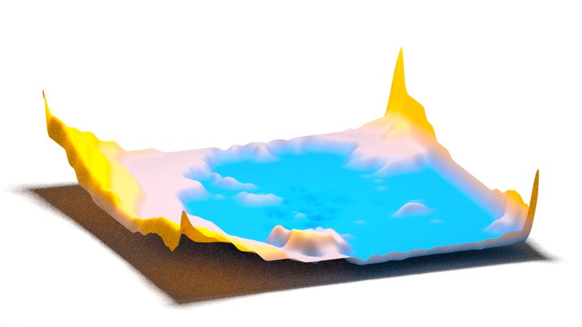
INNAMORATI ET AL.: LEARNING ON THE EDGE                                                           7
Table 1: Quantitative results. Different rows are different tasks. Different columns express
different measures and different methods. Absolute error is measured using different metrics
(eventually not identical to the loss), while the Error ratio is expressed as the ratio of the loss
of our method over the opposing boundary rules. Best is bold. The architecture used for these
tests is described in Sec. 4.
                                     Absolute error                  Error ratio
                                      Other metric                   MSE ratio
       Task         Src      Unit    refl zero          Ours     refl zero       Ours
  Gauss filtering          DSSIM      .0018    .0022    .0016    79 %     83 %     100 %
 De-noise/Bayer     [7]     PSNR      31.46    31.50    31.94    90 %     89 %     100 %
   Colorization     [15]   DSSIM      .1593    .1604    .1577    99 %     98 %     100 %
      Disparity     [5]        px     1.538    1.511    1.403    84 %     88 %     100 %
     Scene flow     [5]        px     1.380    1.183    1.096    56 %     73 %     100 %

    Additionally, we propose to measure the success as the loss ratio between the test loss of
our architecture with and the test loss of an architecture without explicit boundary handling,
using the MSE metric. We suggest to use the ratio as it abstracts away from the unit and the
absolute loss value that depends on the task, allowing to compare effectiveness across tasks.

5.2    Results
Gauss blur Gauss filtering is a simple baseline task with little relevance to any practical
application as we know the solution (Sec. 4.) It is relevant to our exposition, as we know that,
if the network had seen the entire world (and not just the image content) it would be able to
solve the task. It is remarkable, that despite the apparent simplicity of the task – it is a single
linear filter after all – the absolute loss is significant enough to be visible for classic boundary
handling. It is even more surprising, that the inability to learn a simple Gauss filter does not
only result in artifacts along the boundaries, but also in the interior. This is to be attributed
to the inability of a linear filter to handle the boundary. In other words, a network without
explicit boundary handling is unable to learn a task as easy as blurring an image. We will see
that this observation can also be made for more complex tasks in the following sections.

De-noising and De-bayering In this application we learn a mapping from noisy images
with a Bayer pattern to clean images using the training data of Gharbi et al. [7]. The measure
is the PSNR, peak signal-to-noise ratio (more is better). We achieve the best PSNR at 31.94,
while the only change is the boundary handling. In relative terms, traditional boundary
handling can achieve only up to 90 % of MSE.

Colorization Here we learn the mapping from grey images to color images using data
from Zhanget al. [15]. The metric again is DSSIM. We again perform slightly better in both
absolute and relative terms.

Disparity and scene flow Here we learn the mapping from RGB images to disparity and
scene flow using the data from Dosovitskiyet al. [5]. We measure error in pixel distances (less
is better). Again, adding our boundary handling improves both absolute and relative error. In
particular, the error of reflect and zero is much higher for scene flow.
8 INNAMORATI ET AL.: LEARNING ON THE EDGE
zero reflect natural Error histogram
C C C
A A A
B B B
Gauss
C C C
Colorization
C C C
A A A
De-bayering
B B B
B B B
Disparity
C C C
Optical flow
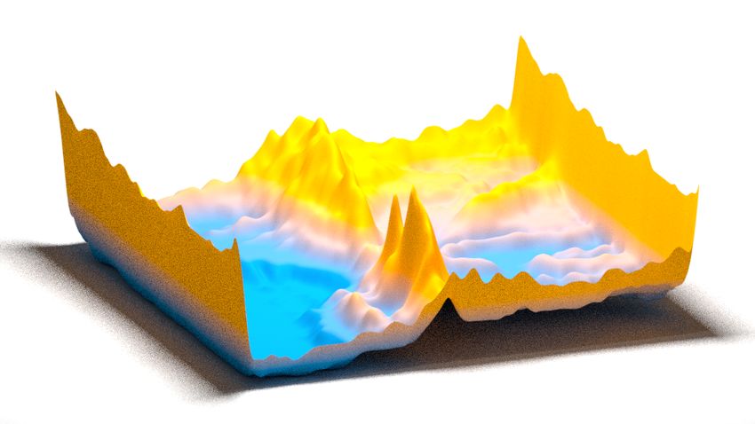
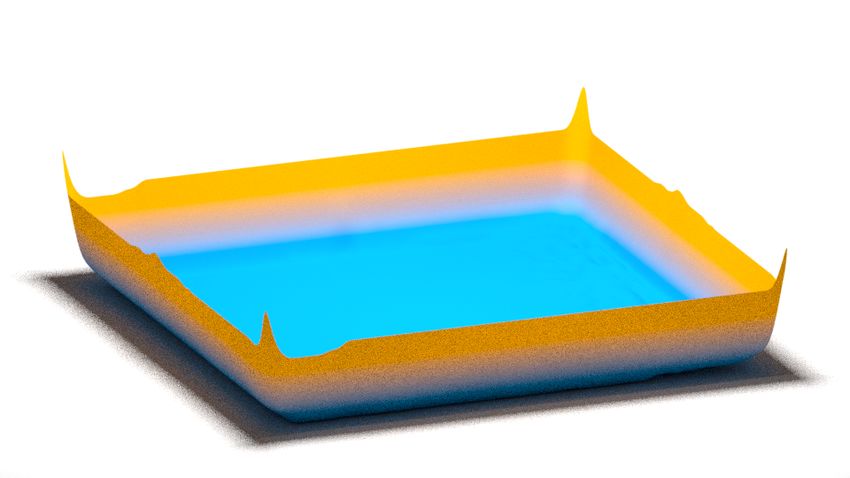
Figure 4: Mean errors across the corpus visualized as height fields for different tasks and
different methods. Each row corresponds to one task each column to one way of handling the
boundary. Arrow A marks the edge that differs (ours has no bump on the edge). Arrow B
mark the interior that differs (ours is flat and blue, others is non-zero, indicting we improve
also inside). Arrow C shows corners, that are consistently lower for us.
6 Discussion
We now will discuss the benefit and challenges of explicit boundary handling.
Overhead Here we study four implementation alternatives for Sec. 3. They were imple-
mented as a combination of OpenGL geometry and fragment shaders. The test was ran on a
Nvidia Gefore 480, on a 3 mega-pixel image and a 3×3 receptive field.
The first method uses a simple zero-padding provided by OpenGL’s sampler2D, in-
voking the GS once to cover the entire domain and applying the same convolution everywhere.
This requires 2.5 ms. This is an upper bound for any convolution code.
The second implementation executes nine different convolutions, requiring 22.5 ms. This
invokes the GS nine times, each invoking all pixels.
The third variant invokes the GS once and a conditional statement for all pixels selects
the kernel weights per-pixel in the domain. This requires 11.2 ms.
The fourth variant, a domain decomposition, invokes the GS nine times to draw nine
quads that cover the respective interior and all boundary cases as seen in recall Fig. 2. Even
after averaging a high number of samples, we could not find evidence for this to be slower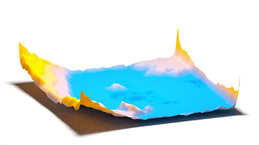
INNAMORATI ET AL.: LEARNING ON THE EDGE                                                          9

than the baseline method i. e., 2.5 ms. This is not unexpected, as the running time for a few
boundary pixels is below the variance of the millions of interior pixels.
     In practice, the learning is limited by other factors such as disk-IO. Our current implemen-
tation in Keras [1], offers a simple form of domain decomposition. We tested the performance
loss over epochs with an average duration of 64 seconds. Our method results in a 0.2%̇
average performance loss over the classic zero rule.

Scalability in receptive field size For small filters, the number of cases is small, but grows
for larger filters. Fortunately, the trend is to rather cascade many small filters in deeper
network, instead of shallower networks with large filters.

Structure Here we seek to understand where spatially in the image the differences are
strongest. While our approach changes the processing on edges, does it also affect the
interior? We compute the per-pixel MAE and average this over all images in the corpus. The
resulting error images are seen in Fig. 4. We found the new method to consistently improve
results in the interior regions. It looks as if the new boundary rules effectively “shield” the
inner regions from spurious boundary influences. The results at the boundaries are very
competitive too, often better than zero and reflect boundary handling. Note, that it is
not expected for any method, also not ours, to have a zero error at the boundary: this would
imply we were able to perfectly predict unobserved data outside of the image.

                                 Convergence Convergence of both our approach and tradi-
        .1          zero         tional zero boundary handling is seen in Fig. 5. We find,
                    reflect
       .01                       that our method is not only resulting in a smaller loss, but
                    explicit
                                 also does so at the same number of epochs. Before we have
Loss

                                 established that the duration of epoch are the same for both
  .001
                                 methods. We conclude there is no relevant training overhead
                                 for our method.
.0001
             0   Epoch     100

                                  Practical alternatives There are simpler alternatives to han-
Figure 5: Convergence rate dle boundaries in an image of n pixels. We will consider a
                                                                      p
with different types of bound- 1D domain as an example here. The first is to crop n pixels
                                                                                            c
ary handling.                     on each side and compute only np − 2nc output pixels. The
cropping nc is to be made sufficiently large, such that no result is affected by a boundary pixel
and nc depends on the network structure. In a single-resolution network of depth nd with a
receptive field size of 2nr + 1, we see, that nc = nd × nr . In a multi-resolution network however,
                                         n
the growth is exponential, so nc = nr d , and for a typical encoder-decoder that proceeds to
a resolution of 1 × 1, every pixel is affected. This leaves two options: either the minimal
resolution is capped and the CNN is applied in a sliding window fashion [11], computing
always only the unaffected result part, incurring a large waste of resources, or the network
simply has to use its own resources to make do with the inconsistent input it receives.

7            Conclusion
In traditional image processing, the choice of boundary rule was never fully satisfying. In
this work, we provide evidence, that CNNs offer the inherent opportunity to jointly extract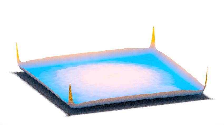
10                                        INNAMORATI ET AL.: LEARNING ON THE EDGE

features and handle the boundary as if the image continues naturally. We do this by learning
filters that are executed on the boundary along with traditional filters executed inside the
image. Incurring little learning and no execution overhead, the concept is simple to integrate
into an existing architecture, which we demonstrate by increased result fidelity for a typical
encoder-decoder architecture on practical CNN tasks.

8    Acknowledgements
We thank Paul Guerrero, Aron Monszpart and Tuanfeng Yang Wang for their technical help
in setting up and fixing the machines used to carry out the experiments in this work. This
work was partially funded by the European Union’s Horizon 2020 research and innovation
programme under the Marie Skłodowska-Curie grant agreement No 642841, by the ERC
Starting Grant SmartGeometry (StG-2013-335373), and by the UK Engineering and Physical
Sciences Research Council (grant EP/K023578/1).

References
 [1] François Chollet et al. Keras. https://keras.io, 2015.
 [2] Dan Ciregan, Ueli Meier, and Jürgen Schmidhuber. Multi-column deep neural networks
     for image classification. In CVPR, pages 3642–49, 2012.
 [3] Taco Cohen and Max Welling. Group equivariant convolutional networks. In ICML,
     pages 2990–9, 2016.
 [4] Jia Deng, Wei Dong, Richard Socher, Li jia Li, Kai Li, and Li Fei-fei. Imagenet: A
     large-scale hierarchical image database. In CVPR, 2009.
 [5] A. Dosovitskiy, P. Fischer, E. Ilg, P. Häusser, C. Hazırbaş, V. Golkov, P. v.d. Smagt,
     D. Cremers, and T. Brox. Flownet: Learning optical flow with convolutional networks.
     In ICCV, 2015.
 [6] Kunihiko Fukushima and Sei Miyake. Neocognitron: A self-organizing neural network
     model for a mechanism of visual pattern recognition. In Competition and cooperation
     in neural nets, pages 267–85. Springer, 1982.
 [7] Michaël Gharbi, Gaurav Chaurasia, Sylvain Paris, and Frédo Durand. Deep joint
     demosaicking and denoising. ACM Trans. Graph., 35(6):191, 2016.
 [8] Ian Goodfellow, Yoshua Bengio, Aaron Courville, and Yoshua Bengio. Deep learning,
     volume 1. MIT press Cambridge, 2016.
 [9] Alex Krizhevsky, Ilya Sutskever, and Geoffrey E Hinton. Imagenet classification with
     deep convolutional neural networks. In NIPS, pages 1097–1105, 2012.
[10] Jimmy SJ Ren, Li Xu, Qiong Yan, and Wenxiu Sun. Shepard convolutional neural
     networks. In NIPS, pages 901–09, 2015.
[11] Olaf Ronneberger, Philipp Fischer, and Thomas Brox. U-net: Convolutional networks
     for biomedical image segmentation. In International Conference on Medical image
     computing and computer-assisted intervention, pages 234–41, 2015.
INNAMORATI ET AL.: LEARNING ON THE EDGE 11
[12] Olga Russakovsky, Jia Deng, Hao Su, Jonathan Krause, Sanjeev Satheesh, Sean
Ma, Zhiheng Huang, Andrej Karpathy, Aditya Khosla, Michael Bernstein, Alexan-
der C. Berg, and Li Fei-Fei. ImageNet Large Scale Visual Recognition Chal-
lenge. International Journal of Computer Vision (IJCV), 115(3):211–252, 2015. doi:
10.1007/s11263-015-0816-y.
[13] Jonas Uhrig, Nick Schneider, Lukas Schneider, Uwe Franke, Thomas Brox, and Andreas
Geiger. Sparsity invariant cnns. arXiv:1708.06500, 2017.
[14] Daniel E. Worrall, Stephan J. Garbin, Daniyar Turmukhambetov, and Gabriel J. Brostow.
Harmonic networks: Deep translation and rotation equivariance. In CVPR, 2017.
[15] Richard Zhang, Phillip Isola, and Alexei A Efros. Colorful image colorization. In ECCV,
2016.You can also read