Level 2 processor and auxiliary data for ESA Version 8 final full mission analysis of MIPAS measurements on ENVISAT
←
→
Page content transcription
If your browser does not render page correctly, please read the page content below
Atmos. Meas. Tech., 15, 1871–1901, 2022
https://doi.org/10.5194/amt-15-1871-2022
© Author(s) 2022. This work is distributed under
the Creative Commons Attribution 4.0 License.

Level 2 processor and auxiliary data for ESA Version 8 final full
mission analysis of MIPAS measurements on ENVISAT
Piera Raspollini1 , Enrico Arnone2,3 , Flavio Barbara1 , Massimo Bianchini4 , Bruno Carli1 , Simone Ceccherini1 ,
Martyn P. Chipperfield5,6 , Angelika Dehn7 , Stefano Della Fera1,8 , Bianca Maria Dinelli2 , Anu Dudhia9 ,
Jean-Marie Flaud10,18 , Marco Gai1 , Michael Kiefer11 , Manuel López-Puertas12 , David P. Moore13,14 ,
Alessandro Piro15 , John J. Remedios13,14 , Marco Ridolfi16 , Harjinder Sembhi14 , Luca Sgheri17 , and Nicola Zoppetti1
1 Istituto di Fisica Applicata Nello Carrara, Consiglio Nazionale delle Ricerche (IFAC-CNR), 50019 Sesto Fiorentino, Italy
2 Istituto di Scienze dell’Atmosfera e del Clima, Consiglio Nazionale delle Ricerche (ISAC-CNR), 40129 Bologna, Italy
3 Department of Physics, University of Turin, 10125 Turin, Italy
4 Istituto dei Sistemi Complessi, Consiglio Nazionale delle Ricerche (ISC-CNR), Section of Florence,

Via Madonna del Piano 10, 50019 Sesto Fiorentino, Italy
5 School of Earth and Environment, University of Leeds, Leeds LS2 9JT, UK
6 National Centre for Earth Observation (NCEO), University of Leeds, Leeds LS2 9JT, UK
7 ESA-ESRIN, 00044 Frascati, Italy
8 Department of Physics and Astronomy, University of Bologna, 40127 Bologna, Italy
9 Department of Physics, University of Oxford, Oxford OX1 3PU, UK
10 Laboratoire Interuniversitaire des Systèmes Atmosphériques (LISA), UMR CNRS 7583, Université de Paris,

Université Paris-Est, 94010 Créteil, Paris, France
11 Karlsruhe Institute of Technology, Institute of Meteorology and Climate Research, Karlsruhe, Germany
12 Instituto de Astrofísica de Andalucía, CSIC, 18008 Granada, Spain
13 National Centre for Earth Observation (NCEO), University of Leicester, Leicester LE4 5SP, UK
14 School of Physics and Astronomy, University of Leicester, Leicester LE1 7RH, UK
15 SERCO SpA c/o European Space Agency ESA-ESRIN, 00044 Frascati, Italy
16 Istituto Nazionale di Ottica, Consiglio Nazionale delle Ricerche (INO-CNR), 50019 Sesto Fiorentino, Italy
17 Istituto per le Applicazioni del Calcolo, Consiglio Nazionale delle Ricerche (IAC-CNR), Section of Florence,

Via Madonna del Piano 10, 50019 Sesto Fiorentino, Italy
18 Institut Pierre-Simon Laplace, 61 avenue du Général de Gaulle, 94010 Créteil CEDEX, France

Correspondence: Piera Raspollini (p.raspollini@ifac.cnr.it) and Marco Gai (m.gai@ifac.cnr.it)

Received: 4 August 2021 – Discussion started: 6 September 2021
Revised: 10 January 2022 – Accepted: 24 January 2022 – Published: 28 March 2022

Abstract. High quality long-term data sets of altitude-          of the processing chain, from the modelling of the measure-
resolved measurements of the atmospheric composition are         ments with the handling of the horizontal inhomogeneities
important because they can be used both to study the evolu-      along the line of sight to the use of the optimal estimation
tion of the atmosphere and as a benchmark for future mis-        technique to retrieve the minor species, from a more sen-
sions. For the final ESA reprocessing of MIPAS (Michelson        sitive approach to detecting the spectra affected by clouds
Interferometer for Passive Atmospheric Sounding) on EN-          to a refined method for identifying low quality products.
VISAT (ENViromental SATellite) data, numerous improve-           Improvements in the modelling of the measurements were
ments were implemented in the Level 2 (L2) processor Op-         also obtained with an update of the used spectroscopic data
timised Retrieval Model (ORM) version 8.22 (V8) and its          and of the databases providing the a priori knowledge of
auxiliary data. The implemented changes involve all aspects      the atmosphere. The HITRAN_mipas_pf4.45 spectroscopic

Published by Copernicus Publications on behalf of the European Geosciences Union.
1872                                                          P. Raspollini et al.: MIPAS L2 v8 processor and auxiliary data

database was finalised with new spectroscopic data verified        as a function of altitude at high vertical resolution. This is
with MIPAS measurements themselves, while recently mea-            mainly driven by the step of the measurement tangent altitude
sured cross-sections were used for the heavy molecules. The        grid and can reach for most trace species the values of 2–3 km
Level 2 Initial Guess (IG2) data set, containing the clima-        in the altitude range 6–40 km, with better performance in the
tology used by the MIPAS L2 processor to generate the ini-         second phase of the mission (see Sect. 2), where the measure-
tial guess and interfering species profiles when the retrieved     ment grid is finer. Middle infrared spectra contain features of
profiles from previous scans are not available, was improved       numerous species: CO2 , used for temperature retrieval; wa-
taking into account the diurnal variation of the profiles de-      ter vapour; ozone and many other longer-lived greenhouse
fined using climatologies from both measurements and mod-          gases; species of interest for ozone chemistry; many nitrogen
els. Horizontal gradients were generated using the ECMWF           and sulfur compounds; gases produced by biomass burning
ERA-Interim data closest in time and space to the MIPAS            and other pollution plumes; and some isotopologues.
data. Further improvements in the L2 V8 products derived              The analysis of MIPAS measurements is performed in two
from the use of the L1b V8 products, which were upgraded           steps: from the interferograms measured by the instrument,
to reduce the instrumental temporal drift and to handle the        the Level 1b (L1b) analysis (Kleinert et al., 2007, 2018)
abrupt changes in the calibration gain. The improvements in-       produces the geolocated and radiometrically calibrated spec-
troduced into the ORM V8 L2 processor and its upgraded             tra. These are then injected into the Level 2 (L2) processor,
auxiliary data, together with the use of the L1b V8 products,      which, starting from these spectra, retrieves the concentration
lead to the generation of the MIPAS L2 V8 products, which          of the atmospheric parameters of interest. The inversion pro-
are characterised by an increased accuracy, better temporal        cedure is based on the simulation (with a full-physics model)
stability and a greater number of retrieved species.               of all atmospheric emission spectra of a limb scan measured
                                                                   by the instrument (computed assuming known atmospheric
                                                                   parameters and information on the instrument response) and
                                                                   on the determination of the atmospheric profiles which min-
1   Introduction                                                   imise the differences between the modelled observations and
                                                                   the real observations. The quality of MIPAS L2 products de-
Atmospheric composition is changing due to the anthro-             pends upon the quality of the L1b products and on the accu-
pogenic emissions of greenhouse gases and pollutants, the          racy of the L2 processor in modelling the observations, tak-
reduction of the ozone-depleting substances regulated by the       ing care that all systematic errors are minimised. The activ-
Montreal Protocol and natural variability, including solar ac-     ities related to the improvements of the L1b and L2 analy-
tivity, volcanic eruptions and pyrocumulonimbus events aris-       ses advanced in parallel during the MIPAS mission, but with
ing from wildfires. Taken together, these changes affect the       large cross-fertilisation between them: detected anomalies in
whole atmosphere from the surface to the thermosphere and          the L2 products motivated investigation into and improve-
largely vary in time, altitude and latitude. High quality long-    ments to the L1b products; changes in the L1b products were
term data sets of global altitude-resolved atmosphere com-         also verified while looking at their impact on the L2 products.
position measurements are essential to understand the in-          The ESA (European Space Agency) L2 processor, based on
teraction between the changes in atmospheric composition           the Optimised Retrieval Model (ORM) algorithm described
and circulation and their impact on climate (IPCC, 2021),          in Ridolfi et al. (2000) and Raspollini et al. (2006), was orig-
weather (see e.g. Kidston et al., 2015) and air quality (see       inally designed to perform near-real-time (NRT) analysis of
e.g. Wang and Fu, 2021). Furthermore, they can be used as a        the MIPAS measurements, with the requirement of a pro-
benchmark for future missions.                                     cessing time of less than 3 h to allow for assimilation of the
   MIPAS (Michelson Interferometer for Passive Atmo-               products by ECMWF (European Centre for Medium-Range
spheric Sounding) was a Fourier transform spectrometer             Weather Forecasts; Dragani, 2012; Thépaut et al., 2012).
(FTS) used for the measurement of atmospheric composition             The end of the mission did not stop the work on improv-
at altitudes from the upper troposphere to the thermosphere,       ing the data, and two sets of full mission reprocessing were
with a special focus on the stratosphere. It was one of few        performed: one with the MIPAS Level 2 Processor Prototype
instruments that allowed for the vertically resolved sounding      (ML2PP) code Version 6 (V6; Raspollini et al., 2013) using
of the infrared emission of the atmosphere over a long period      L1b V5 data, and the second with ML2PP V7 (De Laurentis
(Fischer et al., 2008). It operated on board the ENVISAT           et al., 2016; Valeri et al., 2017) with L1b V7 data. These two
satellite in a sun-synchronous polar orbit for 10 years, tak-      sets of ESA reprocessing were performed with improvements
ing measurements from July 2002 to April 2012. It observed         to the original NRT algorithm, but other independent L2 re-
the atmospheric emission at the limb in the middle infrared        processing was also performed (Dinelli et al., 2010; Dudhia,
spectral region, allowing for continuous measurement during        2008; Kiefer et al., 2021).
both day and night. The sequence of limb observations at dif-         For the final reprocessing of the whole MIPAS mission, a
ferent tangent altitudes provides information about the con-       significant effort was made by the MIPAS Quality Working
centration of the constituents emitting in the middle infrared     Group, supported by ESA, to further improve both L1b and

Atmos. Meas. Tech., 15, 1871–1901, 2022                                             https://doi.org/10.5194/amt-15-1871-2022
P. Raspollini et al.: MIPAS L2 v8 processor and auxiliary data                                                              1873

L2 processors, as well as spectroscopy and a priori knowl-         was the line of sight’s azimuth commanded to the poleward
edge of the atmosphere. The objective was to obtain L2 prod-       side of the flight path. A very small fraction of the measure-
ucts with increased accuracy, reduced instrumental temporal        ments were performed looking sideways on the side opposite
drift, reduced discontinuities in the time series and a greater    to the Sun to explore the possibility of aircraft emission mea-
number of retrieved species.                                       surements (for a sketch of the measurement geometry, see
   The improvements implemented in the L1b V8 processor            Fig. 5 of Fischer et al., 2008).
are described in Kleinert et al. (2018), where the error esti-        With an orbit period of 100.6 min, 14.3 orbits d−1 were
mate of the L1b products is also provided. Here we focus on        performed. The quasi-polar orbit allowed for global cover-
the description of the main features and recent changes im-        age, with MIPAS covering almost the whole globe in 3 days.
plemented in ORM version 8.22 (used for the final full mis-        The instrument has two input ports (one receives the ra-
sion reprocessing and referred to in the rest of the paper as      diation from the atmosphere and the other is designed to
ORM V8 or ESA L2 processor V8), which also includes the            look at a cold target in order to minimise its contribution
use of L1b V8 products. Each implemented improvement is            to the energy load on the detectors) and two output ports,
discussed by analysing its impact on the quality of L2 prod-       each of them equipped with four detectors (A1 to D1 and
ucts. Some of the improvements implemented in the L1b pro-         A2 to D2 for the two ports, respectively) centred at dif-
cessor are also briefly recalled with the intent of highlighting   ferent wavenumbers that together cover the spectral range
their direct impact on the quality of the L2 products. The de-     from 685 to 2410 cm−1 . The spectra from the eight detec-
scription of the implemented improvements is meant to bet-         tors are combined in five spectral bands (denoted A, 685–
ter understand the products of this processor and to inspire       980 cm−1 ; AB, 1010–1180 cm−1 ; B, 1205–1510 cm−1 ; C,
future developers of retrieval codes.                              1560–1760 cm−1 ; D, 1810–2410 cm−1 ) in the L1b products.
   The paper is organised as follows. In Sect. 2 the MIPAS,        The long-wavelength channels A1, A2, B1 and B2 use pho-
onboard the ENVISAT satellite, and the characteristics of the      toconductive mercury cadmium telluride (MCT) detectors,
measurements are briefly recalled, while in Sect. 3 the main       while photovoltaic MCT detectors are used in the short wave-
characteristics of the retrieval program implemented in the        length channels C1, C2, D1 and D2.
L2 processor and its auxiliary data are discussed. The sub-           In the first 2 years of operation (from July 2002 to March
sequent three sections are dedicated to the description of the     2004), MIPAS acquired, nearly continuously, measurements
improvements in the L2 analysis; in particular, Sect. 4 is ded-    at full spectral resolution (FR), with a maximum interfero-
icated to the changes in the modelling of the measurements,        metric optical path difference (MOPD) of 20 cm, correspond-
including the use of an updated spectroscopic database and         ing to an FTS spectral resolution of δσ = 1/(2 × MOPD) =
state-of-the-art knowledge of the atmosphere for the defi-         0.025 cm−1 . A spectrum at this spectral resolution is mea-
nition of initial guess and a priori profiles. Section 5 deals     sured in 4.5 s. On 26 March 2004, FR measurements were
with changes that make possible the retrieval of very minor        discontinued due to a mechanical problem in the interfer-
species, and Sect. 6 deals with the choices adopted to reduce      ometer drive unit. After the detection of this anomaly, on
the number of outliers in the products. Section 7 describes        the basis of in-flight tests, a new safe value of 8 cm was
the impact of improvements implemented in the L1b V8 data          established for the MOPD. With this new MOPD, an un-
on the reduction of both the instrument drift and the error        apodised spectral resolution δσ = 0.0625 cm−1 is achieved,
in the radiometric calibration; Sect. 8 deals with the changes     with a total time of 1.8 s required for the measurement of a
in the format of the output files. Finally, the conclusions are    limb spectrum. The savings in measurement time were then
given in Sect. 9.                                                  exploited both to implement a finer vertical sampling of the
                                                                   atmospheric limb and to acquire additional limb scans within
                                                                   each orbit. Atmospheric measurements with these character-
2   MIPAS on ENVISAT mission                                       istics were resumed in January 2005. Due to this optimised
                                                                   (more dense) spatial sampling, the measurements acquired
MIPAS measured atmospheric limb emission spectra on                from January 2005 onward are referred to as optimised reso-
board the ENVISAT satellite launched by ESA in 2002 (Fis-          lution (OR) measurements.
cher et al., 2008). Flying at about 800 km with a near-circular       The nominal FR (OR) scan pattern consists of 17
polar sun-synchronous orbit inclined of 98.55◦ with respect        (27) sweeps with tangent heights in the range from 6 to 68 km
to the plane of the Equator, it overpassed each region on          (from 5–12 km to 70–77 km according to latitude) with 3 km
Earth at the constant local time of 10:00/22:00, with the day-     (1.5 km) steps in the upper troposphere–lower stratosphere
side measurements being performed during the descending            (UTLS) region. It should be noted that, associated with the
part of the orbit (from north to south) and the nightside mea-     change of the measurement vertical grid occurring in the OR
surements during the ascending one.                                phase, this grid became floating; i.e. the grid moved rigidly
   MIPAS was installed at the rear of ENVISAT, looking             following the lowest tangent altitude determined at each lat-
backwards with respect to the satellite’s flight direction. Only   itude according to a latitude-dependent law in order to better
around the poles, in order to get a better latitude coverage,      follow the tropopause height and to have at least one sweep

https://doi.org/10.5194/amt-15-1871-2022                                            Atmos. Meas. Tech., 15, 1871–1901, 2022
1874                                                           P. Raspollini et al.: MIPAS L2 v8 processor and auxiliary data

below the tropopause. Hence the covered altitude range is              Instrument effects are also taken into account. The instru-
5–70 km in the polar region, 7.05–72.05 km at 45◦ and 12–           ment line shape (ILS) and the instantaneous field of view
77 km at the Equator. Further details are provided in Dinelli       (IFOV) are modelled using an accurate instrument character-
et al. (2021).                                                      isation (Fischer et al., 2008). Scattering is not included in the
   Beyond the nominal measurement modes described above,            radiative transfer integral, and the spectra affected by thick
which are used for most MIPAS measurements in both                  clouds, identified by a cloud filtering algorithm (Spang et al.,
phases of the mission, other measurement modes were ac-             2002, 2004; Raspollini et al., 2006), are not considered in the
quired and processed. Some are focused on the UTLS re-              analysis.
gion, some on the middle atmosphere and some on the upper              The atmosphere is assumed to be in local thermodynamic
atmosphere. Both horizontal and vertical sampling vary for          equilibrium (LTE) and in hydrostatic equilibrium. The im-
the different measurement modes. The horizontal sampling            pact of unaccounted for atmospheric effects (non-LTE, in-
varies from 550 km in the first phase of the mission to about       terfering species, etc.) is minimised through the selection of
410 km in the second phase for the nominal mode, but there          spectral intervals (microwindows) containing relevant infor-
are measurements modes where it is even smaller. Further de-        mation on target parameters and minimising the systematic
tails of the characteristics of the MIPAS measurement modes         errors (Dudhia et al., 2002; Dudhia, 2019). Furthermore, re-
are contained in Dinelli et al. (2021) and references therein.      trievals are performed only up to 78 km as a maximum. Other
Almost all measurement modes are processed by the ESA               algorithms which take non-LTE into account (see e.g. López-
processor.                                                          Puertas et al., 2018, and references therein) perform the anal-
                                                                    ysis for the whole mesosphere and the lower thermosphere.
                                                                       Mutual interference of species that contribute to the same
3   Review of theoretical baseline of the L2 algorithm              spectral region is handled with individual constituents re-
                                                                    trieved according to an order of spectroscopic relevance. In
The ORM Level 2 processor (Ridolfi et al., 2000; Raspollini
                                                                    this way the main interfering species are modelled with a
et al., 2006, 2013) was specifically designed to operate in
                                                                    concentration that has been previously derived from the same
NRT and to use a minimum amount of a priori information
                                                                    atmospheric sample. The only exception to the sequential re-
that may introduce a bias in the profiles. To this end, the al-
                                                                    trieval is the case of the pressure corresponding to the tan-
titude grid of the retrieval coincides with the tangent points
                                                                    gent altitudes and the related temperature values (p, T re-
of the limb measurements (or a subset of them) where the
                                                                    trieval). These two quantities are retrieved simultaneously
sensitivity of the measurements peaks. The retrieval is per-
                                                                    exploiting the external information provided by the hydro-
formed using the global fit method (Carlotti, 1988), consist-
                                                                    static equilibrium and the engineering knowledge of the limb
ing of the simultaneous fit of the whole limb scanning se-
                                                                    scanning steps. Then the altitude grid is rebuilt starting from
quence of the spectra acquired at different tangent altitudes.
                                                                    the lowest engineering tangent altitude corrected using in-
The non-linear least-squares fit is used and the chi-square
                                                                    formation from co-located ECMWF altitude/pressure pro-
(χ 2 ) is minimised using the Gauss–Newton approach with
                                                                    files (see Raspollini et al., 2013 and Dinelli et al., 2021).
an iterative procedure. The ill-conditioned problem of the
                                                                    Therefore, for each scan, the first operation is the simulta-
measurements is handled with the regularising Levenberg–
                                                                    neous p, T retrieval, followed by a sequential retrieval of
Marquardt approach (Levenberg, 1944; Marquardt, 1963;
                                                                    the trace gases’ volume mixing ratio (VMR) profiles (first
Hanke, 1997; Doicu et al., 2010) during the iterations and
                                                                    H2 O, then O3 and then all the other species). The retrieval
with an a posteriori regularisation with a self-adapting con-
                                                                    vector includes, in addition to the species (or p, T ) pro-
straint dependent on the random error of each profile (Cec-
                                                                    file, microwindow-dependent continuum transmission pro-
cherini, 2005; Ridolfi and Sgheri, 2011) applied after con-
                                                                    files and microwindow-dependent but height-independent
vergence. An accurate method, specifically designed for the
                                                                    offset calibration values. The improvements implemented in
regularising Levenberg–Marquardt approach, is used for the
                                                                    the L2 processor ORM V8 involve both the forward and in-
computation of the diagnostic quantities (covariance matrix,
                                                                    verse models, as well as the approach for filtering out spectra
CM; averaging kernel matrix, AKM; Ceccherini and Ridolfi,
                                                                    affected by clouds and for filtering out profiles with bad qual-
2010). The forward model internal to the retrieval code sim-
                                                                    ity.
ulates the atmospheric radiance measured by the spectrom-
eter as the result of the radiative transfer in a non-uniform
medium. In the early versions the medium was non-uniform
in the vertical direction, while it was assumed to be uniform       4   Improvements in the modelling of the measurements
in the horizontal direction, i.e. along the line of sight. Since
                                                                    As stated above, the retrieval of atmospheric parameters from
V8 of the processor (see Sect. 4.1), horizontal gradients of
                                                                    MIPAS remote sensing measurements requires the fit of the
temperature and trace gases have been taken into account
                                                                    simulated measurements to the observations through an itera-
along the line of sight.
                                                                    tive procedure. The fit is performed through the minimisation
                                                                    of the chi-square function, defined as the weighted L2 norm

Atmos. Meas. Tech., 15, 1871–1901, 2022                                              https://doi.org/10.5194/amt-15-1871-2022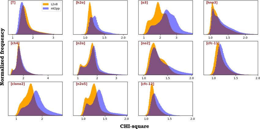
P. Raspollini et al.: MIPAS L2 v8 processor and auxiliary data                                                                    1875

Figure 1. Chi-square distribution of all FR NOM L2 V8 (orange) and L2 V7 (blue) profiles for some representative trace species.

of the residuals (given by the difference between the obser-           a double peak that corresponds to the different impact of in-
vations and the simulations), with the weight given by the in-         terference of non-target gases in the various latitude bands
verse of the CM of the observations. The chi-square function           explored by the measurements along the orbits. For most of
is then normalised with the number of degrees of freedom               the retrieved gases we observe a reduction in the V8 chi-
of the fit (i.e. the number of observations minus the num-             square as compared to V7, indicating a better representation
ber of the retrieved parameters). If optimal estimation (see           of the observations. This improvement is more significant in
Sect. 5.1) is used, the function to be minimised also takes            the OR phase of the mission, where the reduced spectral res-
into account the constraints imposed to the retrieval, namely          olution makes the interference of non target gases more crit-
the square differences between the retrieved parameters and            ical. The retrievals characterised by the largest reduction in
the a priori parameters, weighted by the corresponding a pri-          the chi-square are H2 O (−8 %), O3 (−20 %), HNO3 (−5 %),
ori error.                                                             N2 O (−5 %), NO2 (−7 %), CFC-12 (−6 %), N2 O5 (−9 %)
   Any effort in improving the modelling of the measure-               and ClONO2 (−14 %). According to the results of dedicated
ments helps in reducing the systematic errors, and this leads          sensitivity tests (not presented here), the obtained chi-square
to a better accuracy of the products. These improvements fo-           reduction is mainly due to the modifications in the building
cused on three main aspects:                                           of the profiles of the gases that spectrally interfere with the
                                                                       target gas (see Sect. 4.3). The improved spectroscopic data
  – the handling of the horizontal inhomogeneities along               used in V8 (see Sect. 4.2) and the introduced horizontal gra-
    the line of sight in the forward model;                            dient model (see Sect. 4.1) also contribute, albeit to a lesser
                                                                       extent, to the observed chi-square decrease.
  – the use of more accurate spectroscopic parameters and
    cross-sections for heavy molecules;
                                                                       4.1   Model of the horizontal variability
  – the use of the state-of-the-art representation of the atmo-
    sphere for defining initial guess profiles, assumed pro-           Systematic differences between profiles retrieved from the
    files of the interfering species and horizontal gradients.         measurements acquired in the day and the night parts of the
                                                                       satellite orbit were observed, for species for which a diurnal
   The overall impact of these modifications on the mod-               variability is not expected, in the L2 products V7 and ear-
elling of the observations can be evaluated in terms of the            lier. As described in Sect. 2, with the only exception of high-
reduction of the chi-square with respect to the previous pro-          latitude measurements for which the illumination depends on
cessing version. Figures 1 and 2 compare the chi-square his-           the season, in the MIPAS data set day/night differences are a
tograms of some representative trace gas retrievals obtained           synonym for descending/ascending differences.
from V7 and V8 L2 data sets, for MIPAS FR and OR nomi-                    Systematic day/night differences were first noted by
nal measurements, respectively. Most of the histograms show            Kiefer et al. (2010), who compared zonal averages of MI-

https://doi.org/10.5194/amt-15-1871-2022                                                  Atmos. Meas. Tech., 15, 1871–1901, 2022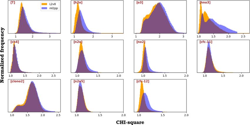
1876                                                            P. Raspollini et al.: MIPAS L2 v8 processor and auxiliary data

Figure 2. Chi-square distribution of all OR NOM L2 V8 (orange) and L2 V7 (blue) profiles for some representative trace species.

PAS measurements owing to the ascending and to the de-                 sults of previous L2 MIPAS/ESA data processing and the
scending parts of the satellite orbit. The observed differences        IG2 database (see Sect. 4.3.1), which includes the climato-
are of the order of the retrieval noise error; therefore they          logical variability with latitude. Sensitivity tests have shown
are only visible when averages of large data sets are com-             that the HGs determined on the basis of the climatological
pared. Kiefer et al. (2010) attributed this effect to the missing      latitude variability tabulated in the IG2 database do not lead
model of the horizontal variability of the atmosphere within           to significant reductions of the ascending/descending differ-
the radiative transfer code. In fact, assuming a linear varia-         ences in the L2 products.
tion of the atmospheric state parameters with latitude, a given           Since the horizontal resolution of MIPAS was of the or-
north–south gradient has opposite-in-sign projections along            der of the horizontal separation between the measured limb
the instrument line of sight, depending on whether the mea-            scans (von Clarmann et al., 2009b), one may argue that at-
surement is acquired in the ascending or in the descending             mospheric variabilities at smaller scales should contribute to
part of the orbit. As a consequence, a forward model as-               the individual measurements with a signal smaller than or of
suming a horizontally homogeneous atmosphere will simu-                the order of the noise. According to this reasoning, we tried
late radiances affected by opposite-in-sign systematic errors          to determine effective HG estimates from the differences be-
in the ascending and in the descending parts of the orbit. In          tween profiles retrieved from adjacent MIPAS scans in ear-
turn, this forward model error will be mapped into system-             lier reprocessing (with the assumption of horizontal homo-
atic overestimates/underestimates of the mean retrieved pro-           geneity). These HGs were actually found to reduce markedly
files in the ascending/descending sections of the orbit. As-           the ascending/descending differences in the L2 products. An-
cending/descending differences were shown (Kiefer et al.,              other estimate of HGs could be determined on the basis of
2010) to vanish when adopting a full tomographic retrieval             the ECMWF profiles. We associated the closest ECMWF
approach (Carlotti et al., 2001), confirming the need to take          profile in space and in time with each MIPAS limb scan.
into account the horizontal variability. Extensive tests (Kiefer       HGs were then determined from the differences between the
et al., 2010; Castelli et al., 2016) showed that modelling the         ECMWF profiles associated with the adjacent limb scans.
horizontal variability of the atmosphere with an externally            The HGs computed with this approach were found to reduce
supplied horizontal gradient (HG) could significantly reduce           the ascending/descending differences exactly as the HGs de-
the systematic mean ascending/descending differences, pro-             termined from previous MIPAS reprocessing. Considering
vided that a proper effective gradient estimate is used. Ac-           that profiles retrieved in earlier MIPAS reprocessing (V7
cording to these results the ORM was modified so that, start-          and earlier) may sporadically show unphysical oscillations,
ing from V8, it models a height-dependent HG of both tem-              for the V8 reprocessing we decided to use HGs determined
perature and gas VMR. HGs are not retrieved; they are com-             on the basis of the ECMWF data set. Specifically, from the
puted from external profile databases. The allowed profile             ECMWF data set, we determined the HGs of temperature,
data sources are the ECMWF database (see Sect. 4.3.2), re-             H2 O and O3 . The HGs of the other gases were set to zero.

Atmos. Meas. Tech., 15, 1871–1901, 2022                                                  https://doi.org/10.5194/amt-15-1871-2022
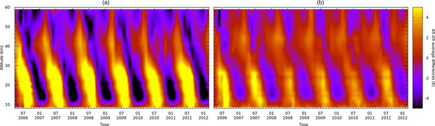
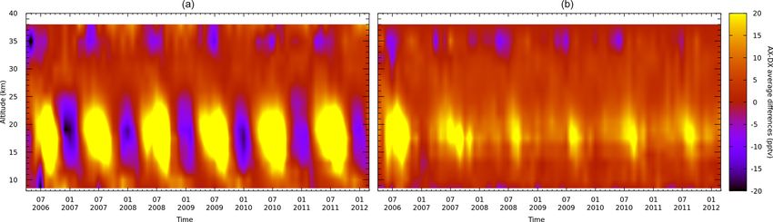
P. Raspollini et al.: MIPAS L2 v8 processor and auxiliary data                                                                  1877

Figure 3. Temperature ascending–descending average difference profiles for V7 (blue) and V8 (red) MIPAS/ESA products. Averaging
extends to the measurements acquired in the month of December of the years 2006 to 2011 (OR part of the mission). The different panels
show different latitude bands as indicated on the top of the panels.

   The HGs are calculated as difference quotients at fixed al-       largest ascending/descending differences. Figures 3 and 4
titudes along the orbit plane. For each scan, we apply the gra-      show the average vertical profiles of ascending/descending
dient to the atmosphere up to a distance δOC from the tangent        differences for temperature and CFC-11, respectively. The
point, where OC (orbital coordinate) is the polar coordinate         averaging period covers the measurements acquired in the
in the orbit plane. We set δOC as the average inter-scan dis-        months of December of the years 2006 to 2011 (i.e. the OR
tance (about 4◦ ). Since the actual angular distance between         part of the mission). The differences were binned into 10 lat-
scans differs from scan to scan, corrective actions have been        itude intervals. We see that, in general, for temperature and
taken to avoid unphysical extrapolations of the atmospheric          CFC-11 the ascending/descending differences in V8 prod-
fields in the OC domain.                                             ucts (red curves) are significantly smaller than in V7 products
   Removing the assumption of horizontal homogeneity of              (blue curves). Specifically, the introduced HG model reduces
the atmosphere implies that Snell’s law could not be ex-             the temperature systematic differences (by about 1 to 2 K)
ploited any longer at the edge of the atmospheric layers, as         at mid- to higher latitudes, while preserving the real ascend-
in the earlier ORM versions. As a consequence, a new ray-            ing/descending (night/day) differences at the tropics, due to
tracing algorithm has been developed in order to calculate           solar tides.
the Curtis–Godson (Curtis, 1952; Godson, 1953) integrals,               The systematic ascending/descending differences are
defining the equivalent quantities of each layer and allow-          linked to the meridional variability of the atmosphere and,
ing for relatively coarse discretisation of the atmosphere (Ri-      therefore, as expected, they depend on the season. The sea-
dolfi et al., 2000). The new ray-tracing algorithm (Ridolfi and      sonality of these differences is illustrated in Figs. 5 and 6.
Sgheri, 2014) solves the eikonal equation in Cartesian coor-         For a selected latitude band (45–60◦ S), these figures show
dinates using a multi-step predictor–corrector method, with          the time series of the monthly average temperature (Fig. 5)
an adaptive step that depends on the curvature of the ray-           and CFC-11 (Fig. 6) ascending/descending difference pro-
paths.                                                               files for V7 (left panel) and V8 (right panel). Although still
   Temperature and CFC-11 were identified by Kiefer et al.           visible, the seasonality of the ascending/descending differ-
(2010) as the most critical target parameters, showing the           ences is much less pronounced in V8 data as compared to

https://doi.org/10.5194/amt-15-1871-2022                                               Atmos. Meas. Tech., 15, 1871–1901, 2022
1878                                                             P. Raspollini et al.: MIPAS L2 v8 processor and auxiliary data

Figure 4. CFC-11 ascending–descending average difference profiles for V7 (blue) and V8 (red) MIPAS/ESA products. Averaging extends to
the measurements acquired in the month of December of the years 2006 to 2011 (OR part of the mission). The different panels show different
latitude bands as indicated on the top of the panels.

Figure 5. Time series of monthly average temperature ascending–descending difference profiles for V7 (a) and V8 (b) MIPAS/ESA products.
The images cover the latitude band from 45 to 60◦ S.

V7. The remaining seasonality in latitude band averages of             4.2   Updated spectroscopic data
V8 measurements could be due to the fact that our model
of the horizontal variability of the atmosphere is a first-order       Full-physics modelling of the measurements requires the
model with a gradient, i.e. we only model an inter-scan lin-           knowledge of the spectroscopic parameters of the trace
ear variation of the atmospheric state. Un-modelled smaller-           species emitting in the spectral region to be simulated. In-
scale atmospheric variabilities, while contributing with a sig-        deed, errors in the spectroscopic parameters are estimated to
nal below the noise in the individual measurements, could              provide one of the major contributions to the total error bud-
cause a visible effect in the averages.                                get of the retrieved profiles (Dudhia, 2019). The crucial role
                                                                       played by the quality of spectroscopy in the quality of re-

Atmos. Meas. Tech., 15, 1871–1901, 2022                                                  https://doi.org/10.5194/amt-15-1871-2022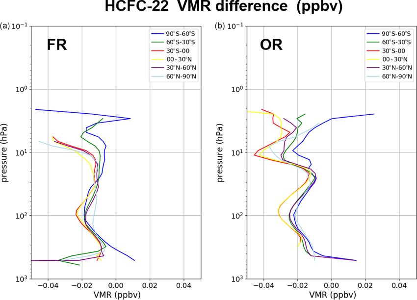
P. Raspollini et al.: MIPAS L2 v8 processor and auxiliary data                                                                1879

Figure 6. Time series of monthly average CFC-11 ascending–descending difference profiles for V7 (a) and V8 (b) MIPAS/ESA products.
The images cover the latitude band from 45 to 60◦ S.

trieved profiles has motivated the development of a dedicated      CFC-114, CFC-115, CCl4 , ClONO2 , N2 O5 , HNO4 and SF6 .
spectroscopic database for MIPAS with an activity that pro-        Among these, new cross-sections have been used in ORM
ceeded in parallel with the development of the L2 processor.       V8 for CFC-12, CFC-14, HCFC-22, CCl4 , ClONO2 , HNO4 ,
For the analysis with ORM V8, the MIPAS dedicated spec-            taken from HITRAN 2016 (Rothman et al., 2017), CFC-11
troscopic database HITRAN_mipas_pf4.45 was used, which             (Harrison, 2018), CFC-113 (Le Bris et al., 2011) and SF6
is the evolution of the HITRAN_mipas_pf3_2 spectroscopic           (Driddi et al., 2022).
database used for the processing of V6 and V7 L2 data sets.           It is important to note that MIPAS measurements them-
The format of the spectroscopic database pf4.45 is compliant       selves were used for some molecules to verify that the new
with HITRAN 2004.                                                  spectroscopic parameters obtained by laboratory measure-
   HITRAN_mipas_pf4.45 is based on HITRAN08 (Roth-                 ments allowed for the reduction of the differences between
man et al., 2009), but spectroscopic parameters for the            observed and simulated spectral features and, thanks to the
molecules O2 , SO2 , OCS, CH3 Cl, C2 H2 and C2 H6 are taken        broadband spectra of MIPAS, checking of the consistency of
from HITRAN 2012 (Rothman et al., 2012). The spectro-              the line parameters of a given molecule in its different ab-
scopic parameters of HNO3 were derived by Perrin et al.            sorption bands. This is the case for HNO3 , for which an ab-
(2016), and the spectroscopic data for COCl2 were derived          solute intensity calibration was performed to “convert” the
by Tchana et al. (2015). Both HNO3 and COCl2 data are now          relative line intensities at 7.6 µm to absolute intensities. This
contained in HITRAN 2016 (Gordon et al., 2017). Spectro-           was done by comparing the HNO3 VMR profiles retrieved
scopic data for the new molecule C3 H8 (Flaud et al., 2010;        from the MIPAS radiances in either the 7.6 or 11 µm regions.
Nixon et al., 2009), which are not present in the HITRAN           A multiplicative factor was applied to all the line intensi-
data set up to 2016, have been included in the pf4.45 data         ties at 7.6 µm so that in the height range of the HNO3 VMR
set. Among the species for which spectroscopic data have           peak (21–24 km), the VMR retrieved using the 7.6 µm inter-
changed significantly with respect to the previous MIPAS           val matched the one retrieved using the 11 µm region, leading
spectroscopic database, HITRAN_mipas_pf3_2, we have to             to better consistency between the 11 and 7.6 µm regions (Per-
mention HCN (see Sect. 4.2.2). Spectroscopic line data rela-       rin et al., 2016).
tive to HOBr are still excluded from the database as the avail-       In Figs. 7, 8 and 9 three examples are shown of spectral
able data are for pure rotational transitions and are outside      intervals selected for the retrieval of HNO3 , COF2 and CFC-
the MIPAS bands. Line data relative to CF4 are also still ex-      12 VMR, where differences in the residuals come from the
cluded from the database since their quality is very poor.         changed spectroscopic data only. It is evident that the use of
   For molecules which exhibit very dense line-by-line spec-       the new spectroscopic database and the new cross-sections
tra that are extremely difficult to model, or for which the        significantly reduces the residuals.
individual transitions have not been assigned, are not accu-
rate enough or are of poor quality, cross-sections measured        Impact on retrieved species
in the laboratory for atmospheric pressure and temperature
ranges are used. It is worth noting that cross-sections also       We have shown some examples of how the use of the new
have the advantage of incorporating various spectroscopic          spectroscopic parameters and cross-sections improves the
effects, such as line coupling and pressure shifts. Measured       spectral simulations of the observations, but they also lead
cross-sections are used for the following molecules: CFC-11,       to significant changes in the retrieved profiles. The valida-
CFC-12, CFC-13, CFC-14, HCFC-21, HCFC-22, CFC-113,                 tion of the retrieved profiles is outside the scope of this pa-

https://doi.org/10.5194/amt-15-1871-2022                                             Atmos. Meas. Tech., 15, 1871–1901, 2022
1880 P. Raspollini et al.: MIPAS L2 v8 processor and auxiliary data
Figure 9. (a) Observed spectrum (black curve, under the blue one)
Figure 7. (a) Observed spectrum (black curve, under the blue and simulations at 15 km with the old and the new spectroscopic pa-
one) and simulations at a limb tangent height of 24 km with the rameters for a microwindow used for CFC-12 retrieval of FR mea-
old (red curve) and the new (blue curve) spectroscopic parame- surements. (b) Residuals obtained with simulations generated with
ters for a microwindow used for HNO3 retrieval of FR measure- the old spectroscopic database (red curve) and the new one (blue
ments. (b) Residuals obtained with simulations generated with the curve), compared with the measurement noise (grey curves).
old spectroscopic database (red curve) and the new one (blue curve),
compared with the measurement noise (grey curves).
Spectroscopic line data updates mostly affect HNO3 , HCN
and COCl2 . The use of the updated spectroscopic database
for HNO3 causes systematically larger profiles between 100
and 10 hPa, with the largest differences being 0.7 (0.2) ppbv
for the FR (OR) measurements around the peak of the profile
in the Antarctic region (see Fig. 10), corresponding to differ-
ences of about +5 % (2.5 %) for the FR (OR) measurements.
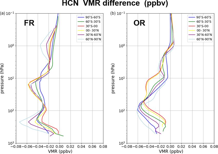
For HCN the changed spectroscopy is responsible for an
even larger difference, greater than 20 pptv between 200 and
10 hPa (see Fig. 11), corresponding to 15 %–20 %. The rea-
son is that a major update has been accomplished for the hy-
drogen cyanide line list since HITRAN 04. Line positions
and intensities throughout the infrared have been revisited
by Maki et al. (1996, 2000). The improvements apply to the
three isotopologues present in HITRAN in the pure rotation
region and in the infrared from 500 to 3425 cm−1 . The new
intensities are about 1.16 times larger than the previous ones.
For the impact of the changes in COCl2 spectroscopy on
Figure 8. (a) Observed spectrum (black curve, under the blue one) the retrieved profiles, we refer the reader to Pettinari et al.
and simulations at 18 km with the old (red curve) and the new (blue (2021).
curve) spectroscopic parameters for a microwindow used for COF2 Systematic differences in the retrieved trace species at-
retrieval of FR measurements. (b) Residuals obtained with simula- tributable to changes in the used cross-sections are found in
tions generated with the old spectroscopic database (red curve) and CCl4 , CFC-11, CFC-12 and HCFC-22 retrieved profiles. In
the new one (blue curve), compared with the measurement noise general, for all the four trace species the new cross-sections
(grey curves).
are characterised by a higher spectral resolution and better
signal-to-noise ratio at low pressure than the previous ones.
The use of the new cross-sections for HCFC-22 (Harrison,
per. Here we only describe the impact of the changes in the 2016) leads, above 200 hPa, to retrieved HCFC-22 VMRs
spectroscopic line data and the cross-sections on the retrieved between 10 and 25 pptv, smaller than with the old cross-
profiles for the most-affected trace species. sections (Prasad Varanasi, private communication, 2000;
Atmos. Meas. Tech., 15, 1871–1901, 2022 https://doi.org/10.5194/amt-15-1871-2022P. Raspollini et al.: MIPAS L2 v8 processor and auxiliary data 1881 Figure 10. Absolute difference between the mean HNO3 profiles retrieved using the new (mipas_pf4.45) and the old (mipas_pf3.2) spec- troscopic databases at different latitude bands for selected orbits in the full resolution (FR) phase (a) and in the optimised resolution (OR) phase (b). Figure 11. Same as Fig. 10, but for the HCN profiles. Clerbaux et al., 1993; see Fig. 12), corresponding to dif- lar, differences can be due to the extended pressure coverage ferences of about 10 %. A possible explanation for this dif- of the new cross-sections. ference is that the Q branches are reasonably sharp, espe- Concerning the other retrieved profiles, V8 CFC-11 VMRs cially near 829 cm−1 , and very sensitive to pressure. So even obtained with the new cross-sections (Harrison, 2018) are though the overall integrated band strength is the quite simi- up to 20–30 pptv smaller than with the old ones (Prasad https://doi.org/10.5194/amt-15-1871-2022 Atmos. Meas. Tech., 15, 1871–1901, 2022
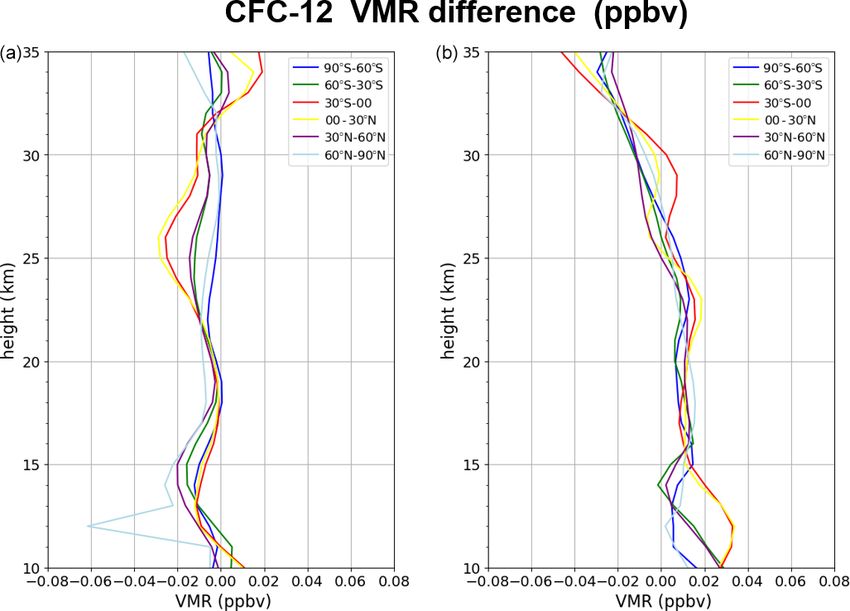
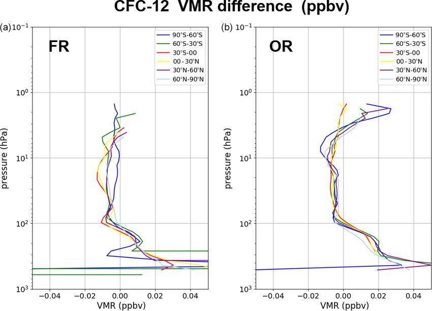
1882                                                         P. Raspollini et al.: MIPAS L2 v8 processor and auxiliary data

Figure 12. Same as Fig. 10, but for the HCFC-22 profiles.

Figure 13. Same as Fig. 10, but for the CFC-11 profiles.

Varanasi, private communication, 2000; see Fig. 13), corre-       new CFC-12 cross-sections (Harrison, 2015) are responsible
sponding to a percent difference of up to 5 %. Differences in     for an increase in the retrieved CFC-12 profiles with respect
CCl4 VMRs retrieved with the new (Harrison et al., 2016)          to the old cross-sections (Prasad Varanasi, private communi-
and the old (Prasad Varanasi, private communication, 2000)        cation, 2000), which is maximal at the lowest altitudes and
cross-sections vary from very small values at 100 hPa for the     equals about 50 pptv; then the difference gradually reduces
tropical bands to −5 to −10 pptv from 200 to 20 hPa for the       with altitude, becoming negligible at 100 hPa, and slightly
other latitude bands and altitudes (see Fig. 14). Finally, the    negative above (Fig. 15).

Atmos. Meas. Tech., 15, 1871–1901, 2022                                           https://doi.org/10.5194/amt-15-1871-2022
P. Raspollini et al.: MIPAS L2 v8 processor and auxiliary data                                                         1883

Figure 14. Same as Fig. 10, but for the CCl4 profiles.

Figure 15. Same as Fig. 10, but for the CFC-12 profiles.

   For CFC-12, it is interesting to compare the differences   mented in the code, produces differences between V8 and V6
in the retrieved profiles between V8 and V6 products with     of the opposite sign in the two phases of the mission (positive
the results of the validation of V6 data with the balloon     in the OR, negative in the FR; Fig. 16), which compensates
BONBON measurements (Engel et al., 2016), which uses          for the bias between MIPAS V6 and BONBON measure-
gas chromatography, for an indirect verification of the im-   ments (negative in the OR, positive in the FR; see Fig. 13
provements implemented in the V8 processor. The use of the    of Engel et al., 2016) leading to a better agreement.
new cross-sections, combined with the other changes imple-

https://doi.org/10.5194/amt-15-1871-2022                                       Atmos. Meas. Tech., 15, 1871–1901, 2022
1884                                                           P. Raspollini et al.: MIPAS L2 v8 processor and auxiliary data

Figure 16. Absolute difference between MIPAS V8 and MIPAS V6 CFC-12 profiles at different latitude bands for selected orbits in FR (a)
and OR (b) phases.

   For the other species validated with the same technique,             – The IG2 data set, consisting of a set of climatologi-
namely CH4 , N2 O and CFC-11 (Engel et al., 2016), the de-                cal profiles of the global atmosphere for six latitude
tected biases of V6 products with respect to BONBON (up                   bands, four seasons (January, April, July and October)
to 300 ppbv at 15 km for FR measurements in CH4 , up to                   and for all years of the MIPAS mission in both nighttime
50 ppbv at 15 km for FR measurements in N2 O and up to                    and daytime conditions. These profiles are available for
40 pptv for CFC-11 in both phases of the mission) were al-                all targets and interfering species in the altitude range
ready partially reduced in V7 products thanks to the use                  0–120 km. The methodology used for generating these
of new N2 O and CH4 microwindows for the analysis of                      data is based on Remedios et al. (2007), and the im-
FR measurements and to the handling of the interference of                provements implemented in version V5.4 (used for the
COCl2 in CFC-11 retrievals (De Laurentis et al., 2016). Fur-              L2 V8 reprocessing) are described in Sect. 4.3.1.
thermore, no significant differences are found in V8 CH4 and
N2 O with respect to the corresponding V7 products, and the             – Profiles from ECMWF ERA-Interim reanalysis that
effect of the new cross-sections for CFC-11 is smaller than               have been chosen for each scan as the closest to MIPAS
the effect of the unaccounted COCl2 interference in V6 CFC-               measurements: this data set includes pressure, temper-
11 profiles.                                                              ature, water vapour and ozone profiles in the altitude
                                                                          range 0–65 km. The way they are selected is described
4.3    Use of a priori knowledge of the atmosphere                        in Sect. 4.3.2.
                                                                        – For the target species, retrieved in sequence from each
In order to perform the retrieval, it is necessary to define the
                                                                          measured scan, the following profiles can also be used,
initial and a priori state of the atmosphere. The atmosphere
                                                                          if available and of “good” quality (see Sect. 6.2): pro-
is described by the vertical distribution of pressure and tem-
                                                                          files from previous retrievals of the current measure-
perature, as well as of the VMR of both the retrieval targets
                                                                          ment scan; retrieved profiles from the previous scan; re-
and the interfering species, and, with the handling of hor-
                                                                          trieved profiles from previous MIPAS reprocessing.
izontal inhomogeneities, also of the horizontal (latitudinal)
gradients of the considered species. The choice of these pro-           Among the different databases, only the IG2 profiles are
files, in particular of the ones which are not target of the re-     available for the altitude range from 0 to 120 km, the others
trieval, is important, because a wrong assumption may intro-         being defined by a restricted altitude range. The extension
duce systematic errors in the retrieved quantities. In general,      of these profiles outside their native range is performed with
the following databases have been developed for defining the         the IG2 profiles which, in order to avoid discontinuities, are
state of the atmosphere.                                             scaled by the ratio between the value of the profile at each

Atmos. Meas. Tech., 15, 1871–1901, 2022                                                https://doi.org/10.5194/amt-15-1871-2022
P. Raspollini et al.: MIPAS L2 v8 processor and auxiliary data 1885
edge of its native altitude range and the corresponding cli- expected for some species. This is done by changing some
matological value interpolated at the same altitude. of the input data sets to accommodate other data sources that
The code uses a priority system to determine the best pos- possess day and night variations. In particular, in the lowest
sible choice for the target species and the interfering species altitude range, the diurnal variation from either the Univer-
(see Dinelli et al., 2021). sity of Leeds SLIMCAT model (see below) or the climatol-
ogy from MIPAS products were implemented into the V5
4.3.1 IG2 data set profile creation procedure, while the IAA data set (see be-
low) was mainly used above this altitude range. The output
The IG2 database (Remedios et al., 2020) consists of the cli- results in two profiles created per gas (per season and per
matological profiles for the following six latitude bands: 90 latitude band) rather than a single mean profile.
to 65◦ N, 65 to 20◦ N, 20◦ N to 0, 0 to 20◦ S, 20 to 65◦ S The University of Leeds SLIMCAT model is a 3D strato-
and 65 to 90◦ S for the four seasons each represented by its spheric chemical transport model that calculates atmospheric
central month January, April, July and October. Profiles are abundances of a number of chemical species (Chipperfield,
represented on a 1 km step vertical grid from 0 km to 120 km 2006). In a combination with TOMCAT, the inclusive TOM-
for pressure (hPa), temperature (K) and volume mixing ra- CAT/SLIMCAT model calculates the global chemical tracer
tios (ppmv) of the following species: N2 , O2 , C2 H2 , C2 H6 , fields from the surface to 80 km for short-lived chemical
C3 H8 , CO2 , O3 , H2 O, CH4 , N2 O, CFC-11, CFC-12, CFC- species, and steady state and source gases, using meteo-
13, CFC-14, CFC-21, HCFC-22, CFC-113, CFC-114, CFC- rological fields from ECMWF. Here, for the stratosphere,
115, CH3 Cl, CCl4 , HCN, NH3 , SF6 , HNO3 , HNO4 , NO, vertical transport is calculated by the CCMRAD (Briegleb,
NO2 , SO2 , CO, HOCl, ClO, H2 O2 , N2 O5 , OCS, ClONO2 , 1992) radiation scheme that encompasses the longwave and
COF2 , COCl2 , HDO and PAN. Daytime and nighttime pro- shortwave radiation domains (from the surface to top-of-
files are provided for the trace gas species that display strong atmosphere). Advection of chemical tracers is performed
diurnal signatures, namely CH4 , ClO, ClONO2 , H2 O, HNO3 , by the Prather scheme (Prather, 1986). A diurnally varying
HNO4 , HOCl, N2 O5 , N2 O, NO2 and O3 . For specific gases SLIMCAT data set was computed specifically for the cre-
(i.e. chlorofluorocarbons and CO2 ), trends are accounted for ation of IG2 diurnally varying profiles. Chemical calcula-
in the IG2 climatology. Although the profiles are tabulated tions were performed on a monthly scale from pre-Pinatubo
only for a limited set of latitude bands and for each season years to years including ENVISAT coverage (1990–2008),
of the years 2002 to 2012 in the IG2 database, discontinu- driven by ECMWF reanalysis, and calculated on a 1 km ver-
ities in the L2 products are avoided by using linear interpo- tical grid extending from the surface to 60 km (1999–2005)
lation. Specifically, for each processed limb scan, the ORM and 80 km (2006–2008). The chemical tracers included in
V8 builds the corresponding IG2 profile estimates by linearly these calculations are O3 , O, O(1 D), N, NO, NO2 , NO3 ,
interpolating the IG2 tabulated profiles to the time and the N2 O5 , HNO3 , ClONO2 , ClO, HCl, HNO4 , HOCl, Cl, Cl2 O2 ,
geolocation of the considered measurement. OClO, Br, BrO, BrONO2 , BrCl, HBr, H2 O2 , HOBr, CO,
The creation of the IG2 profiles follows the methodology CH4 , N2 O, H, OH, HO2 , H2 O, H2 SO4 , CFC-11, CFC-12,
of Remedios et al. (2007), in which several data sources are CH3 Br, CH2 O, HF, COF2 and COFCl. Data are provided as
selected for specific regions of the atmosphere and merged to zonally averaged day and night concentration profiles, zonal
create a full vertical concentration profile from the ground to minimum/maximum day and night profiles and standard de-
120 km. The following data sets are used for the creation of viation day and night profiles. Data are gridded onto a 5◦ lat-
the V5 IG2 profiles: URAP (UARS Reference Atmosphere itude grid ranging from 85◦ S to 85◦ N and on a 1 km vertical
Project) profiles (Remedios, 1998), ACE-FTS on SCISAT grid.
v3.6 data set (Bernath et al., 2003), SLIMCAT model profiles Climatology from MIPAS products was generated for a
(see description below), GEOS-Chem model profiles (Bey et check on diurnal variation provided by SLIMCAT. In partic-
al., 2001 and, for NH3 , Molod et al., 2012), IAA profiles de- ular, MIPAS-Oxford profiles (Dudhia, 2008) were used. A
rived for upper altitudes and diurnal variations as required for Z test filter (Daszykowski et al., 2007) was applied to the
non-LTE calculations (see description below) and mean pro- MIPAS-Oxford data to remove any outliers. Some control
files calculated from ensembles of MIPAS-Oxford profiles tests performed with ORM, consisting of pressure and tem-
(2008–2009) for the MIPAS target species (Dudhia, 2008). perature retrievals for selected orbits covering the four sea-
A summary of the input data used for IG2 V5 profiles is pro- sons, performed using the climatological profiles taken from
vided in Table 1. CFCs and organics are constrained by the either the V4.1 IG2 database or the new diurnally varying
V3 ACE-FTS data set with further filtering to remove neg- IG2 database as the interfering species profiles, revealed that
ative volume mixing ratios. Variable smoothing lengths, de- larger chi-square values were found compared to the V4.1
pending on species and atmospheric lifetime, are required to IG2 database when using N2 O5 profiles derived by SLIM-
smooth out small-scale vertical variability. CAT, with the largest discrepancies in the polar regions. It
For the generation of a day and night data set, the creation was found that the N2 O5 profiles generated by SLIMCAT
of V5 differs only so as to incorporate the diurnal differences did not appear to suitably represent the diurnal variation
https://doi.org/10.5194/amt-15-1871-2022 Atmos. Meas. Tech., 15, 1871–1901, 20221886 P. Raspollini et al.: MIPAS L2 v8 processor and auxiliary data
Table 1. Summary of input data for IG2 V5 profiles. For previous versions, we refer the reader to Remedios et al. (2007). The standard
atmosphere (SA) database is a set of climatological profiles that represent the global atmosphere under conditions of varying atmospheric
state (Remedios et al., 2007). Other data sets used are described in the text.
IG2 species Data source IG2 species Data source
C2 H2 ACE-FTS v3.6 CFC-115 URAP
C2 H6 ACE-FTS v3.6 H2 O MIPAS-Oxford, IAA
C3 H8 ACE-FTS v3.6 H2 O2 URAP, SA
CCl4 ACE-FTS v3.6 HCN ACE-FTS v3.6
CH3 Cl URAP HDO ACE-FTS v3.6
CH4 MIPAS-Oxford, IAA HNO3 MIPAS-Oxford, IAA
ClO URAP, IAA HNO4 SLIMCAT, IAA
ClONO2 MIPAS-Oxford, IAA HOCl SLIMCAT, IAA
CO SLIMCAT, IAA N2 URAP
CO2 URAP, IAA N2 O MIPAS-Oxford, IAA
COCl2 ACE-FTS v3.6 N2 O5 SLIMCAT, IAA
COF2 ACE-FTS v3.6 NH3 GEOS-Chem
CFC-11 ACE-FTS v3.6 NO URAP, IAA
CFC-12 ACE-FTS v3.6 NO2 MIPAS-Oxford, IAA
CFC-13 URAP O2 URAP
CFC-14 ACE-FTS v3.6, URAP O3 MIPAS-Oxford, IAA
CFC-21 URAP OCS ACS-FTS v3.6
HCFC-22 ACE-FTS v3.6, URAP PAN ACS-FTS v3.6, SLIMCAT
CFC-113 ACE-FTS v3.6, URAP SF6 ACS-FTS v3.6, URAP
CFC-114 URAP SO2 URAP, SA
(10:00/22:00) expected for these species, especially in the nal variations, the calculations for particular reference days
polar regions, despite good apparent agreement with the twi- were performed (see Table 2 in López-Puertas et al., 2009)
light occultation observations of ACE-FTS. In the end, mean within the corresponding season (i.e. March–May for April)
profiles calculated from ensembles of MIPAS-Oxford N2 O5 at 10:00/22:00 local time. These reference days were chosen
profiles (2008–2009) were preferred over SLIMCAT profiles such that solar zenith angle (SZA) at 10:00/22:00 reflects the
in defining the diurnal information for generating the V5 average SZA of all MIPAS observations in the corresponding
IG2 profiles. To keep consistency between all of the diurnal latitudinal and seasonal band in day (SZA < 90◦ ) and night
species retrieved by MIPAS, similar V5 IG2 profiles were (SZA > 90◦ ) conditions. The photo-dissociation coefficients,
generated for all operational species (O3 , N2 O, ClONO2 , J , were calculated in the IAA box model with the TUV
H2 O, CH4 , HNO3 and NO2 ). model (Madronich and Flocke, 1998), except for JNO , which
Above 80 km, the IAA data set (López-Puertas, 2009) is was taken from the Minschwaner and Siskind (1993) param-
mainly used. This supplies a set of climatological profiles eterisation. More details on the generation of this data set
extending from the surface up to 200 km for the same six lat- can be found in López-Puertas et al. (2009) and in Sect. 3.1
itude bands, four seasons and nighttime and daytime condi- of Funke et al. (2012).
tions of the IG2 database. For the generation of these profiles,
the SLIMCAT profiles available up to 80 km were extended 4.3.2 ECMWF data set
and/or modified up to 200 km as detailed in Table A1. The
data set contains profiles for (a) pressure and temperature, The ECMWF data set is taken from ECMWF ERA-Interim
which were taken from the IG database version V4 (Reme- (Dee et al., 2011), the latest global atmospheric reanalysis of
dios et al., 2007) below 70 km, and from the MSIS model ECMWF model results available at the start of MIPAS data
(Picone et al., 2002) above that altitude; (b) VMR profiles reprocessing. The data set covers the period 1979 to 2019
for H2 O, CO2 , O3 , N2 O, CO, CH4 , NO, NO2 , HNO3 , OH, with a spatial resolution of approximately 79 km (T255 spec-
ClO, HO2 , O, O(1 D), N, H, N2 , O2 and HCN; and (c) non- tral) over 60 vertical levels from the surface up to 0.1 hPa.
LTE relevant parameters as the photo-dissociation rates of O2 ERA-Interim data include temperature, humidity and ozone
and NO, JO2 and JNO , respectively. profiles, which are made available as 6-hourly atmospheric
To generate this data set, we used a simple 1D chemistry fields.
model (the IAA box model), MSIS model (Picone et al., Data on model levels were adopted instead of pressure lev-
2002), the 2D model of Garcia and Solomon (1994) and the els in order to obtain a greater vertical coverage since they
NOEM (Marsh et al., 2004) for NO. Concerning the diur- are released up to 0.1 hPa (about 65 km altitude) versus 1 hPa
Atmos. Meas. Tech., 15, 1871–1901, 2022 https://doi.org/10.5194/amt-15-1871-2022You can also read