LOCALIZATION OF COCHLEAR IMPLANT ELECTRODES FROM CONE BEAM COMPUTED TOMOGRAPHY USING PARTICLE BELIEF PROPAGATION

Page created by Steven Perez
 
CONTINUE READING
LOCALIZATION OF COCHLEAR IMPLANT ELECTRODES FROM CONE BEAM COMPUTED TOMOGRAPHY USING PARTICLE BELIEF PROPAGATION
LOCALIZATION OF COCHLEAR IMPLANT ELECTRODES FROM CONE BEAM
                                                    COMPUTED TOMOGRAPHY USING PARTICLE BELIEF PROPAGATION

                                                  Hendrik Hachmann?∗                        Benjamin Krüger†             Bodo Rosenhahn?              Waldo Nogueira†
                                                                                        ?
                                                                                 Leibniz University Hanover, Germany
                                                       †
                                                           Department of Otorhinolaryngology, Hannover Medical School, Hanover, Germany
                                                                      †
                                                                        Cluster of Excellence ‘Hearing4All’, Hanover, Germany
arXiv:2103.10434v1 [cs.CV] 18 Mar 2021

                                                                     ABSTRACT
                                         Cochlear implants (CIs) are implantable medical devices that
                                         can restore the hearing sense of people suffering from pro-
                                         found hearing loss. The CI uses a set of electrode contacts
                                         placed inside the cochlea to stimulate the auditory nerve with
                                         current pulses. The exact location of these electrodes may
                                                                                                                      Fig. 1: Comparison of 2 synthetic (a,b) and 2 real (c,d) CBCT
                                         be an important parameter to improve and predict the perfor-
                                                                                                                      data-sets of cochlear implants (CIs). (a) is an example of a
                                         mance with these devices. Currently the methods used in clin-
                                                                                                                      closely-spaced EA, while (b,c,d) represents distantly-spaced
                                         ics to characterize the geometry of the cochlea as well as to
                                                                                                                      EAs. Both synthetic data-sets include a high number of false
                                         estimate the electrode positions are manual, error-prone and
                                                                                                                      positives to evaluate the robustness of localization algorithms.
                                         time consuming.
                                             We propose a Markov random field (MRF) model for CI
                                         electrode localization for cone beam computed tomography
                                                                                                                      oped [1]. A CI consists of an external sound processor and an
                                         (CBCT) data-sets. Intensity and shape of electrodes are in-
                                                                                                                      electrode array (EA). Latter is implanted inside the cochlea,
                                         cluded as prior knowledge as well as distance and angles be-
                                                                                                                      which is a spiral-shaped bone cavity making 2.5 turns around
                                         tween contacts. MRF inference is based on slice sampling
                                                                                                                      its axis with a length that ranges between 32 and 43.5 mm
                                         particle belief propagation and guided by several heuristics.
                                                                                                                      [2]. The EAs are manufactured with lengths ranging from
                                         A stochastic search finds the best maximum a posteriori esti-
                                                                                                                      10 to 31 mm including 12-22 electrode contacts. Long EAs
                                         mation among sampled MRF realizations.
                                                                                                                      may achieve up to two full turns of insertion to reach low-
                                             We evaluate our algorithm on synthetic and real CBCT
                                                                                                                      frequency stimulation [3]. After surgery, CBCT scans are
                                         data-sets and compare its performance with two state of the
                                                                                                                      recorded to determine the position of the EA contacts rela-
                                         art algorithms. An increase of localization precision up to
                                                                                                                      tive to the ear anatomy. This information may be useful for
                                         31.5% (mean), or 48.6% (median) respectively, on real CBCT
                                                                                                                      different relevant tasks when programming or fitting CI de-
                                         data-sets is shown.
                                                                                                                      vices, i.e. it may be useful to deactivate electrodes [4] or to
                                             Index Terms— Automatic localization, Cochlear im-                        reduce their current strength in electric-acoustic stimulation
                                         plant, Markov random fields, Electrode                                       (EAS) subjects [5, 6]. CI arrays use contacts spacing rang-
                                                                                                                      ing from around 0.8 mm to 2 mm. CBCT scanners typically
                                                               1. INTRODUCTION                                        used in the clinical routine have a resolution ranging from
                                                                                                                      0.1 to 0.3 mm3 . This relatively low resolution in relation to
                                         Cochlear implants (CIs) are implantable medical devices that                 the contact spacing together with image reconstruction dis-
                                         are used to restore the sense of hearing for people with pro-                tortions and artifacts in the surrounding of the electrode array
                                         found deafness given that the auditory anatomy is fully devel-               cause that manual localization of individual electrode contacts
                                                                                                                      from CBCT scans becomes inaccurate. This manual labor
                                            ∗ H.H. and B.R. were partly funded by the Lower Saxony Ministry of Sci-
                                                                                                                      is tedious and time consuming and not applicable for large
                                         ence and Culture under grant number ZN 3491 within the Lower Saxony
                                         “Vorab“ of the Volkswagen Foundation and by the Federal Ministry of Ed-      data-sets [7]. For this purpose an automatic method to assess
                                         ucation and Research (BMBF), Germany under the project LeibnizKILabor        electrode location (e.g. [8, 9, 10, 11]) would be very use-
                                         (grant no. 01DD20003) and the Center for Digital Innovations (ZDIN). W.N.    ful, but remains challenging. The main contributions in this
                                         and B.K. received funding for this research from the Deutsche Forschungs-
                                         gemeinschaft (DFG, German Research Foundation) under Germany’s Excel-
                                                                                                                      paper are a synthetic CI data-set generator, the MRF-based
                                         lence Strategy EXC 2177/1 ’Hearing4all’, DFG project numbers 390895286       CI localization algorithm (MRF-A) and its comparison with
                                         and 396932747 (PI: W.N.).                                                    state-of-the-art algorithms.
LOCALIZATION OF COCHLEAR IMPLANT ELECTRODES FROM CONE BEAM COMPUTED TOMOGRAPHY USING PARTICLE BELIEF PROPAGATION
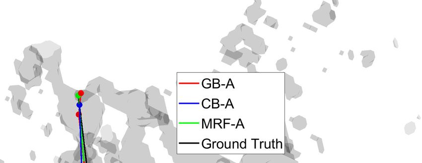
2. STATE-OF-THE-ART                                cal expert using the OsiriX MD software (Pixmeo, Geneva,
                                                                    Switzerland) for 3D reconstruction and visualization.
Two categories of data-sets brought up different strategies to          Similar to Bouix et al. [15] we evaluate algorithms on
automatically locate electrodes from CBCT volumes. The              synthetic data-sets with the advantage that the ground truth
first one contains closely-spaced EAs, i.e. CBCT scans in           (GT) is precisely known. An EA is characterized as a se-
which there is no contrast difference between electrode con-        quence of electrode contacts, each causing high intensity val-
tacts, while vice versa there are distantly-spaced EAs with         ues in CBCT data-sets. Wire leads, receiver coils, and bone
varying intensities between electrode contacts. Noble et al.        structures can have similar appearance, especially in low in-
[12] apply gradient vector flow snakes to locate 3D center-         tensity lCTs [18]. A EA follows a helix structure, due to the
lines (as in [13]), on which the EA is registered by a thin-plate   anatomy of the cochlea. We create synthetic EAs in a two-
spline transformation. Other algorithms use a blob detector as      step procedure: (I) GT electrode positions xn are generated,
Frangi et al. [14] or a surface-based centerline point extrac-      which (II) are used to create a synthetic CBCT volume Isyn .
tion similar to Bouix et al. [15] as a preprocessing step. For          (I) Assume a Cartesian coordinate system with axis
instance, Noble et al. [10] propose a graph-based algorithm         u, v, w. Starting at an initial seed position xn=0 , the EA
that sequentially adds centerline candidates to a growing set       is created by successively adding further electrodes with
of paths, which are than evaluated and pruned to a fixed num-       every iteration n. In
ber of candiates. The predicted EA is refined by a second run
using new candidates sampled from a grid around the previ-            xn+1 (u, v, λ1 · (n + 1)) = xn (u, v, λ1 · n)
ously found EA locations. Braithwaite et al. [9] focused on                    + [cos(λ2 · n · α), sin(λ2 · n · α), 1] · lprior , (1)
the problem of locating distantly-spaced electrode arrays, by
individually locating electrodes in a given volume of interest      lprior is the distance between electrodes and λ2 -weighted α
(VOI). Three filters are sequentially applied: a thresholding       is an angle controlling increasing curvature with n. Thus Eq.
filter, a spherical filter and a Gaussian filter. Detected con-     (1) creates a helix that screws in or out of the u,v-plane as a
tacts are reordered based on a prior knowledge of the type          factor of λ1 . These electrode positions are altered by several
of electrode array. Bennink et al. [8] use a filter which en-       parameters: mirroring (λmirror ∈ {0, 1}) to imitate left or
hances small blob-like structures (Lindeberg [16]), followed        right ear CIs and 3D rotations (θu ,θv ,θw ) for arbitrary orien-
by a curve tracking stage that sequentially includes maximum        tations. These synthetic EA positions are considered GT.
intensity voxels form a predicted VOI. The estimated curve              (II) We create an empty equilateral high resolution syn-
is smoothed and correlation with the CI specifications is con-      thetic volume I0 that comprises all EA contacts positions, also
ducted to estimate the final electrode location. More recently,     adding a guard interval at all borders. 20 electrode positions
Chi et al. [17] used conditional generative adversarial net-        xn and a number of nbones randomly inserted bone-like struc-
works (cGANs) to generate likelihood maps in which voxel            tures xb are added by
values are proportional to the distance to the nearest candidate        I0 (x ∈ {xn ∪ xb }) = 1 ∧ I0 (x ∈
                                                                                                        / {xn ∪ xb }) = 0.         (2)
contact. Using a high threshold on the map, electrode posi-
tions can be extracted. With decreasing threshold, electrodes       I0 is smoothed by a Gaussian filter Gσ1 (·) with standard de-
are merged together, which is tracked and the connection of         viation σ1 , downsampled by S↓ (·) to a target size using cu-
electrodes is found. All preexisting algorithms localize elec-      bic interpolation. Intensities are scaled and shifted by λ3
trodes sequentially, while our approach is the first to jointly     and λ4 and white noise N1 is added to generate Isyn = λ3 ·
optimize all electrode positions, mutual distances and angles.      S↓ (Gσ1 (I0 )) + λ4 + N1 . A diverse CI data-set is generated
                                                                    ([Isyn , GT]-pairs, see Fig 1 and Table 1) using randomly sam-
                                                                    pled parameters (λ1−4 , λmirror , θu−w , αn , σ1 , nbones and
    3. SYNTHETIC AND REAL CBCT DATA-SETS                            N1 ) from suitable ranges. The synthetic data-set and its gen-
                                                                    erator are available1 .
Post-operative temporal bone CBCT scans were collected
from ten CI users denoted as CBCT1 to CBCT10. The CI
users were implanted with a MidScala (CBCT1 and CBCT2)                    4. ELECTRODE ARRAY LOCALIZATION
or a SlimJ (CBCT3 to CBCT10) electrode array (Advanced
                                                                    We propose a MRF-based algorithm (MRF-A), that estimates
Bionics, Valencia, CA). The arrays include 16 electrode con-
                                                                    the 3D positions of electrodes inside a user specified VOI with
tacts that are equally spaced with a distance of approximately
                                                                    the most basal contact marked. The VOI size is around 1 cm3
1 mm. CBCT scans were collected using a Xoran MiniCat
                                                                    and must contain all EA contacts. The MRF model energy is
(Ann Arbor, MI, USA) for CBCT1 and CBCT2 and a 3D
                                                                    defined as
Accuitomo 170 (J. Morita. Mfg. Corp., Kyoto, Japan) for                       X                  X       X
CBCT3 to CBCT10 with an isotropic voxel resolution of                E(x) =           ψs (xs ) +                   ψs,t (xs , xt ), (3)
                                                                                  s∈V                 s∈V     t∈Ns
0.3 mm and 0.125 mm, respectively. The manually determi-
nation of electrode localization was performed by a clini-            1 https://github.com/hendrik-hachmann/synCIg
0.6

                                                                                                                                                 0.5          GB-A (metric a)

                                                                                                         Error (metric a and metric b) [in mm]
                                                                                                                                                              CB-A (metric a)
                                                                                                                                                              MRF-A (metric a)
                                                                                                                                                              GB-A (metric b)
                                                                                                                                                 0.4          CB-A (metric b)
                                                                                                                                                              MRF-A (metric b)

                                                                                                                                                 0.3

Fig. 2: Binary potential in MRF-A: The distance ratio
dst2 /dst1 between nodes xn constrains the angles αn .                                                                                           0.2

                                                                                                                                                 0.1

in which V is a set of nodes with neighbors Ns . The random
variable xs is the 3D position of node s. The unary potential                                                                                     0
                                                                                                                                                       5         10        15
                                                                                                                                                       Electrode number

      ψs (xs ) = Θ1 · Gσ2 (I(xs )) + Θ2 · GBlob (I(xs ))       (4)
                                                                      Fig. 3: Qualitative comparison of the algorithms GB-A (based
takes a CBCT intensities I into account, where Gσ2 (I) is             on [10]), CB-A (based on [8]), MRF-A and the ground truth
a smoothed (Gaussian filter, standard deviation σ2 ) and              (GT) on the data-set CBCT3. The corresponding per electrode
GBlob (I) a blob filter-enhanced version of I. All Θx are             localization errors along the electrode array (EA) are given on
empirically set weighting parameters. The binary potential            the right. Index 1 is the most basal electrode. For CB-A and
                    (                     2                           MRF-A dashed and solid lines run coincidently. In Table 1
                      Θ3 kxs − xt − dst1 k2 for t ∈ N1,s
  ψs,t (xs , xt ) =                                                   metric a) and b) errors are averages per data-set.
                                          2
                      Θ4 kxs − xt − dst2 k2 for t ∈ N2,s
models relationships between node xs and a neighboring node           analytically from the potentials ψs and ψs,t , and particles xns
xt in the EA. The neighborhood N1,s is used to constrain the          are sampled from the uniform distribution UA .
node distance to match the prior known distance dst1 for a                 However, PBP gives the opportunity to encode further CI
specific EA. The second order neighborhood N2,s is used to            a priori knowledge in the form of particle sets that guides the
form an angular constraint as illustrated in Fig. 2. We en-           optimization and improves convergence. In each PBP itera-
force an decreasing angle αn of the EA in apical direction by         tion n, the most likely configuration x̂t is used to augment the
successively reducing the ratio dst2 /dst1 .                                                                           (1)      (p)
                                                                      current slice sampling particle set Pt = {xt , · · · , xt } of
    In order to efficiently minimize the MRF energy (Eq. (3)),        node t containing p particles: Pt,augmented = Pt ∪Pmobility ∪
we approximate the maximum a posterior (MAP) probabil-                PCI ∪ Protated ∪ Pknn . At each PBP iteration, Pmobility
ity using of max-product particle belief propagation (PBP) as         adds the positions x̂t of each direct neighbor to the particle
Pacheco et al. [19]. Following the notation of Besse et al.           set as well as predicted positions at the apical end of the EA,
[20], for a set of particles (i) and PBP iteration n ∈ 1, · · · , N   based on position, length and angle of the two most apical
                                         (i)
we minimize the log disbelief Bsn (xs ) to obtain the most            nodes. In that way, Pmobility provides additional mobility to
                                              (i)
likely configuration x̂s = arg min BsN (xs ) after N itera-           the MRF model in longitudinal direction along the EA. The
tions of belief propagation. Since our binary potential ψs,t          particles sets PCI attempt to predict the whole EA making use
consists of loops (e.g. x1 x2 , x2 x3 , and x1 x3 in Fig. 2) we       of its helix shape. From the positions x̂t , a low energy section
optimize via message passing (Wainwright et al. [21]):                (evaluating Eq. (3)) of 4 to 6 consecutive nodes is extracted,
                              X                                       angles in this sequence are calculated and a helix shape is fit.
   Bsn (x(i)           (i)
          s ) = ψs (xs ) +
                                          n
                                       Mt→s  (x(i)
                                                s ) and               The predicted helix positions are added to PCI . Electrode
                                 t∈Ns
 n                                   n−1          n−1                 positions may be predicted in the wrong way direction, e.g.
Mt→s (x(i)
       s ) = min [ψs,t (xs , xt ) + Bt   (xt ) − Ms→t (xt )].
                xt ∈Pt                                                predicting a clockwise CI counter-clockwise. To encounter
      (i)                                                      (i)
                                                                      this problem, we add Protated to the particle set, a 180 de-
Bsn (xs ) is iteratively calculated by messages Mt→s   n
                                                           (xs )      gree rotated version of x̂t along the vector: basal node x0 to
sent from node t to node s at iteration n.                            center position of x̂t . The particle set Pknn includes the k
    The performance of PBP is heavily dependent on sam-               nearest candidate points, generated by the algorithm of Broix
pling good particles xns from the target log-disbelief distribu-      et al. [15], and thus attracts model towards these locations.
tion xns ∼ Bsn (xs ). Each particle xns is sampled using Markov       The particle set is decimated by diverse particle max-product
                                              (i)
chain Monte Carlo (MCMC) sampling {xs                 }m=1,···,M      [23] to remain constant in size. Due to its stochastic nature,
with m MCMC iterations. We apply slice sampling particle              each optimization of the particle-based MRF can be seen as
belief propagation (S-PBP) as in Müller et al. [22]. Slice sam-      a random walk of the CI model, thus providing different esti-
pling estimates an interval A on the estimated belief distribu-       mates at multiple runs. This can be used in a random search,
tion, which defines a slice u. The interval A can be computed         e.g. run the algorithm Nruns times and take the best solution
Table 1: EA localization score, metric a) and metric b) [in mm] measured for 11 synthetic and 10 CBCT data-sets. On CBCT data-sets, the MRF-A achieves a
                                                                                                  mean score of 0.50 mm, which is 28.6% better than the second best algorithm (median: 0.31 mm, 43.6% increase; 31.5% and 48.6% compared to third method).
                                                                                                  On synthetic data-sets MRF-A achieves a mean score of 0.34, a 44.3% to 54.7% mean and a 56.9% to 63.8% median increase. While most EAs can be classified as
                                                                                                  distantly spaced, the yellow highlighted data-sets have increasingly closer spaced EAs. No data-set has a pure no contrast EA. Average runtimes for MRF-A are 21
in terms of lowest MAP energy. Each MRF run is initialized

                                                                                0.25
                                                                                0.24
                                                                                0.24
                                                                                0.23
                                                                                0.59
                                                                                0.83
                                                                                0.29
                                                                                0.25
                                                                                0.45
                                                                                0.28
                                                                                0.24
                                                                                0.36
                                                                                0.25
                                                                                 b)
at the most basal electrode and pointing randomly inwards the

                                                                                                  minutes (Nruns set to 100), GB-A 2 minutes (α9 = 3 and P = 500) and CB-A 1.4 seconds, using M ATLAB implementations and a Xeon W-2145 processor.
VOI. The current MRF state x̂t can degenerate, e.g. reach a

                                                                     MRF-A
folded prediction of the EA, and no change in MAP energy

                                                                      0.25
                                                                      0.24
                                                                      0.24
                                                                      0.23
                                                                      0.43
                                                                      0.80
                                                                      0.29
                                                                      0.25
                                                                      0.40
                                                                      0.28
                                                                      0.24
                                                                      0.33
                                                                      0.25
                                                                       a)
is detected. In this case we reinitialize ties between electrode
positions by calculating the shortest path between electrodes.

                                                                                score
                                                                                0.25
                                                                                0.24
                                                                                0.24
                                                                                0.23
                                                                                0.51
                                                                                0.82
                                                                                0.29
                                                                                0.25
                                                                                0.43
                                                                                0.28
                                                                                0.24
                                                                                0.34
                                                                                0.25
           5. EXPERIMENTS AND RESULTS

                                                                                1.41
                                                                                0.89
                                                                                3.32
                                                                                0.30
                                                                                0.26
                                                                                1.52
                                                                                0.52
                                                                                0.25
                                                                                1.04
                                                                                1.84
                                                                                0.99
                                                                                1.12
                                                                                0.99
                                                                                 b)
MRF-A is compared with a graph-based algorithm GB-A,

                                                                     CB-A

                                                                     0.39
                                                                     0.58
                                                                     0.51
                                                                     0.30
                                                                     0.26
                                                                     0.41
                                                                     0.37
                                                                     0.25
                                                                     0.30
                                                                     0.35
                                                                     0.38
                                                                     0.37
                                                                     0.37
similar to Noble et al. [10] and with a correlation-based al-

                                                                      a)
gorithm CB-A, similar to Bennink et al. [8]. Parameters of
all algorithms are optimized empirically, for GB-A and CB-A

                                                                                score
                                                                                0.90
                                                                                0.73
                                                                                1.92
                                                                                0.30
                                                                                0.26
                                                                                0.96
                                                                                0.45
                                                                                0.25
                                                                                0.67
                                                                                1.10
                                                                                0.69
                                                                                0.75
                                                                                0.69
starting in the vicinity of the parameters specified in the corre-
sponding papers. We perform the algorithm evaluation based
on two localization error metrics. For each predicted elec-

                                                                                0.92
                                                                                0.43
                                                                                0.72
                                                                                0.64
                                                                                0.70
                                                                                1.61
                                                                                1.61
                                                                                0.87
                                                                                0.64
                                                                                0.43
                                                                                0.86
                                                                                0.86
                                                                                0.72
                                                                                 b)
trode, we calculate the Euclidean distance a) to the nearest GT
electrode position and b) to the GT electrode position with the

                                                                     GB-A

                                                                     0.39
                                                                     0.43
                                                                     0.39
                                                                     0.52
                                                                     0.54
                                                                     0.22
                                                                     0.25
                                                                     0.29
                                                                     0.41
                                                                     0.35
                                                                     0.31
                                                                     0.37
                                                                     0.39
                                                                      a)
same label or electrode number. While metric a) represents a
mean electrode localization error, it does not appropriately re-
flect errors like EA folding, since the folded electrodes can be                score
                                                                                0.65
                                                                                0.43
                                                                                0.55
                                                                                0.58
                                                                                0.62
                                                                                0.91
                                                                                0.93
                                                                                0.58
                                                                                0.52
                                                                                0.39
                                                                                0.58
                                                                                0.61
                                                                                0.58
near other GT positions. Also if the whole predicted EA is
shifted by one electrode, this error is underestimated. Thus,
                                                                     Data-set

                                                                                Median
                                                                                Synth10
                                                                                Synth11
we evaluate on metric b) as well. Using the average of metric
                                                                                Synth1
                                                                                Synth2
                                                                                Synth6
                                                                                Synth8

                                                                                Synth3
                                                                                Synth7
                                                                                Synth9
                                                                                Synth4
                                                                                Synth5
                                                                                Mean
a) and b) we create an overall score. Results can be seen in
Table 1. Although MRF-A needs a lot of computation power,
the EA localization is an automatic task where runtimes are of

                                                                                0.25)
                                                                                0.36
                                                                                1.99
                                                                                0.09
                                                                                0.24
                                                                                0.56
                                                                                2.59
                                                                                0.26
                                                                                0.65
                                                                                0.17

                                                                                         0.72
                                                                                         0.31
minor importance. Fig. 3 presents a comparison of the local-
                                                                                 b)

ization results obtained with the GB-A, CB-A and MRF-A on
                                                                     MRF-A

the CBCT3 data-set, with corresponding errors on metrics a)
                                                                      0.36
                                                                      0.49
                                                                      0.09
                                                                      0.24
                                                                      0.36
                                                                      0.22
                                                                      0.26
                                                                      0.37
                                                                      0.17
                                                                      0.25

                                                                                         0.28
                                                                                         0.25
                                                                       a)

and b) along the EA shown on the right. In this example, all
three algorithms provide a low metric a) scores, while GB-A
                                                                                score
                                                                                0.36
                                                                                1.24
                                                                                0.09
                                                                                0.24
                                                                                0.46
                                                                                1.41
                                                                                0.26
                                                                                0.51
                                                                                0.17
                                                                                0.25

                                                                                         0.50
                                                                                         0.31
has two electrode detections at the most basal electrode, lead-
ing to further electrodes being shifted from the GT and larger
than 0.6 mm metric b) errors. Similar errors can be found for
                                                                                0.73
                                                                                2.00
                                                                                0.16
                                                                                0.27
                                                                                0.83
                                                                                2.34
                                                                                0.27
                                                                                0.32
                                                                                2.54
                                                                                1.07

                                                                                         1.05
                                                                                         0.78
                                                                                 b)

all algorithms in Table 1, indicated by high metric b) values.
                                                                     CB-A

                                                                     0.41
                                                                     0.63
                                                                     0.16
                                                                     0.27
                                                                     0.44
                                                                     0.21
                                                                     0.27
                                                                     0.31
                                                                     0.42
                                                                     0.31

                                                                                         0.34
                                                                                         0.31
                                                                      a)

                      6. CONCLUSION
                                                                                score
                                                                                0.57
                                                                                1.32
                                                                                0.16
                                                                                0.27
                                                                                0.63
                                                                                1.27
                                                                                0.27
                                                                                0.31
                                                                                1.48
                                                                                0.69

                                                                                         0.70
                                                                                         0.60

In this work, we have proposed an MRF-based algorithm
(MRF-A) for CI electrode localization that optimizes the
EA contacts positions by satisfying the CI constraints: high
                                                                                2.06
                                                                                0.41
                                                                                2.16
                                                                                0.24
                                                                                0.34
                                                                                0.52
                                                                                1.85
                                                                                0.32
                                                                                1.20
                                                                                2.76

                                                                                         1.19
                                                                                         0.86
                                                                                 b)

CBCT intensity and blob-shape of electrodes, distance and
angle between electrodes as well as angle increase in apical
                                                                     GB-A

                                                                     0.33
                                                                     0.40
                                                                     0.13
                                                                     0.24
                                                                     0.34
                                                                     0.16
                                                                     0.28
                                                                     0.32
                                                                     0.20
                                                                     0.28

                                                                                         0.27
                                                                                         0.28

direction. The particle-based optimization is guided by sev-
                                                                      a)

eral CI-adapted heuristics to increase convergence. Using the
                                                                                mean

stochastic nature of MRF-A, we created a pool of candidate
                                                                                1.19
                                                                                0.41
                                                                                1.15
                                                                                0.24
                                                                                0.34
                                                                                0.34
                                                                                1.06
                                                                                0.32
                                                                                0.70
                                                                                1.52

                                                                                         0.73
                                                                                         0.55

EAs and the best candidate is selected. We compared our
algorithms with two implementations based on state-of-the-
                                                                                CBCT10
                                                                     Data-set

art algorithms (GB-A, CB-A) using synthetic data-sets, for
                                                                                         Median
                                                                                CBCT1
                                                                                CBCT2
                                                                                CBCT3
                                                                                CBCT4
                                                                                CBCT5
                                                                                CBCT6
                                                                                CBCT7
                                                                                CBCT8
                                                                                CBCT9

                                                                                         Mean

which a precise GT is known, and real CBCT data-sets from
10 subjects. Two metrics show that MRF-A is robust and
achieves low error rates.
7. COMPLIANCE WITH ETHICAL STANDARDS                            [11] Y. Zhao, B. M. Dawant, R. F. Labadie, and J. H. Noble,
                                                                       “Automatic localization of closely spaced cochlear im-
This is a numerical simulation study for which no ethical ap-          plant electrode arrays in clinical cts,” Medical Physics,
proval was required.                                                   vol. 45, no. 11, pp. 5030–5040, 2018.

                                                                  [12] J. Noble, T. Schuman, C. Wright, R. Labadie, and
                    8. REFERENCES
                                                                       B. Dawant, “Automatic identification of cochlear im-
                                                                       plant electrode arrays for post-operative assessment,”
 [1] T. Lindeberg, C. C. Finley, D. T. Lawson, R. D. Wolford,
                                                                       Proc SPIE Med Imaging, vol. 796217, 03 2011.
     D. K. Eddington, and W. M. Rabinowitz, “Better speech
     recognition with cochlear implants,” Nature, vol. 352,       [13] H. Hachmann, M. Awiszus, and B. Rosenhahn, “3d
     no. 6332, pp. 236–238, 1991.                                      braid guide hair reconstruction using electroluminescent
                                                                       wires,” Vis. Comput., 2018.
 [2] W. Würfel, H. Lanfermann, T. Lenarz, and O. Majdani,
     “Cochlear length determination using cone beam com-          [14] A. F. Frangi, W. J. Niessen, K. L. Vincken, and M. A.
     puted tomography in a clinical setting,” Hearing Re-              Viergever, “Multiscale vessel enhancement filtering,”
     search, vol. 316, pp. 65 – 72, 2014.                              MICCAI, pp. 130–137, 1998.
 [3] I. Hochmair, E. Hochmair, P. Nopp, M. Waller, and            [15] S. Bouix, K. Siddiqi, and A. Tannenbaum, “Flux driven
     C. Jolly, “Deep electrode insertion and sound coding in           automatic centerline extraction,” Medical Image Analy-
     cochlear implants,” Hearing Research, vol. 322, 2014.             sis, vol. 9, no. 3, pp. 209 – 221, 2005.
 [4] Y. Zhao, B. M. Dawant, and J. H. Noble, “Automatic           [16] T. Lindeberg, “Scale-space theory: A basic tool for
     selection of the active electrode set for image-guided            analysing structures at different scales,” Journal of Ap-
     cochlear implant programming image-guided cochlear                plied Statistics, vol. 21, pp. 224–270, 09 1994.
     implant programming,” Journal of Medical Imaging,
     vol. 3, no. 3, 2016.                                         [17] Y. Chi, J. Wang, Y. Zhao, J. Noble, and B. Dawant,
                                                                       “A deep-learning-based method for the localization of
 [5] M. Imsiecke, B. Krüger, A. Büchner, T. Lenarz, and              cochlear implant electrodes in ct images,” ISBI, 2019.
     W. Nogueira, “Electric-acoustic forward masking in
     cochlear implant users with ipsilateral residual hearing,”   [18] Y. Zhao, S. Chakravorti, R. F. Labadie, B. M. Dawant,
     Hearing Research, vol. 364, pp. 25 – 37, 2018.                    and J. H. Noble, “Automatic graph-based method for
                                                                       localization of cochlear implant electrode arrays in clin-
 [6] B. Krüger, A. Büchner, and W. Nogueira, “Simultane-             ical ct with sub-voxel accuracy,” Medical Image Analy-
     ous masking between electric and acoustic stimulation             sis, vol. 52, pp. 1 – 12, 2019.
     in cochlear implant users with residual low-frequency
     hearing,” Hearing Research, vol. 353, 06 2017.               [19] R. Kothapa, J. Pacheco, and E. Sudderth, “Max-product
                                                                       particle belief propagation,” Brown University, 2011.
 [7] H. Hachmann, P. Faltin, T. Kraus, and K. Chaisaowong,
     “3d-segmentierungskorrektur unter berücksichtigung          [20] F. Besse, C. Rother, A. Fitzgibbon, and J. Kautz, “Pmbp:
     von bildinformationen für die effiziente und objektive           Patchmatch belief propagation for correspondence field
     erfassung pleuraler verdickungen,” in Bildverarbeitung            estimation,” BMVC, 2012.
     für die Medizin, Mar. 2013, pp. 296–301.                    [21] M. J. Wainwright, T. S. Jaakkola, and A. S. Will-
 [8] E. Bennink, J. P. M. Peters, A. W. Wendrich, E. Vonken,           sky, “MAP estimation via agreement on (hyper)trees:
     G. A. van Zanten, and M. A. Viergever, “Automatic lo-             Message-passing and linear programming,” CoRR, vol.
     calization of cochlear implant electrode contacts in ct.,”        abs/cs/0508070, 2005.
     Ear and hearing, vol. 38 6, pp. e376–e384, 2017.             [22] O. Müller, M. Y. Yang, and B. Rosenhahn, “Slice sam-
                                                                       pling particle belief propagation,” ICCV, 2013.
 [9] B. Braithwaite, H. M. Kjer, J. Fagertun, M. A. G.
     Ballester, A. Dhanasingh, P. Mistrik, N. Gerber, and         [23] J. Pacheco and E. Sudderth,   “Proteins, particles,
     R. R. Paulsen, “Cochlear implant electrode localization           and pseudo-max-marginals: A submodular approach,”
     in post-operative ct using a spherical measure,” ISBI,            ICML, 2015.
     2016.

[10] J. H. Noble and B. M. Dawant, “Automatic graph-based
     localization of cochlear implant electrodes in ct,” MIC-
     CAI, pp. 152–159, 2015.
You can also read