Macroeconomic Outcomes and COVID-19: A Progress Report - Brookings Institution
←
→
Page content transcription
If your browser does not render page correctly, please read the page content below
BPEA Conference Drafts, September 24, 2020

Macroeconomic Outcomes and COVID-19: A
Progress Report

Jesús Fernández-Villaverde, University of Pennsylvania
Charles I. Jones, Stanford University

    DO NOT DISTRIBUTE – ALL PAPERS ARE EMBARGOED UNTIL 9:00PM ET 9/23/2020
of Interest
Conflict of InterestDisclosure:
Disclosure: The authors
Disclosure: The authors did not receive financial support from from any
any firm
firm or
or person
personfor
forthis
this
paper or
paper or from
fromanyanyfirm
firmororperson
personwith
with a financial
a financial or or political
political interest
interest in this
in this paper.
paper. TheyThey are currently
are currently not an
not officers,
officer, director,
directors, ormembers
or board board member
of any of any organization
organization with anwith an interest
interest in this in this paper.
paper.Macroeconomic Outcomes and COVID-19:
A Progress Report
Jesús Fernández-Villaverde Charles I. Jones⇤
UPenn and NBER Stanford GSB and NBER
September 13, 2020 — Version 0.5
Abstract
This paper combines data on GDP, unemployment, and Google’s COVID-19 Com-
munity Mobility Reports with data on deaths from COVID-19 to study the macroe-
conomic outcomes of the pandemic. We present results from an international per-
spective using data at the country level as well as results for individual U.S. states
and key cities throughout the world. The data from these different levels of geo-
graphic aggregation offer a remarkably similar view of the pandemic despite the
substantial heterogeneity in outcomes. Countries like Korea, Japan, Germany, and
Norway and cities such as Tokyo and Seoul have comparatively few deaths and low
macroeconomic losses. At the other extreme, New York City, Lombardy, the United
Kingdom, and Madrid have many deaths and large macroeconomic losses. There
are fewer locations that seem to succeed on one dimension but suffer on the other,
but these include California and Sweden and potentially offer useful policy lessons.
⇤
We are grateful to Andy Atkeson and Jim Stock for many helpful comments and discussions...MACROECONOMIC OUTCOMES AND COVID-19 1
1. Introduction
This paper combines data on GDP, unemployment, and Google’s COVID-19 Commu-
nity Mobility Reports with data on deaths from COVID-19 to study the macroeconomic
outcomes of the pandemic. We present results from an international perspective us-
ing data at the country level as well as results for individual U.S. states and key cities
throughout the world.
The evidence to date can be summarized in a stylized way by Figure 1. On the
horizontal axis is the number of deaths (per million population) from COVID-19. The
vertical axis shows a cumulative measure of the macroeconomic losses apart from the
value of the loss in life; for simplicity here we call this the “GDP loss.” Throughout this
paper, we will show data for various countries, U.S. states, and global cities to fill in this
graph quantitatively. We will also show the dynamics of how countries traverse through
this space over time. For now, though, we simply summarize in a stylized way our main
findings.
Figure 1: Summary of the Trade-off Evidence
GDP LOSS
New York City
Lombardy
California
[lucky? too tight?] United Kingdom
Madrid
[unlucky? bad policy?]
Germany, Norway
Japan, S. Korea
China, Taiwan Sweden
[unlucky? too loose?]
Kentucky, Montana
[lucky? good policy?]
COVID DEATHS
One can divide the graph into four quadrants, based on many versus few deaths
from COVID-19 and on large versus small losses in GDP. Our first interesting finding is
that there are communities in all four quandrants.
In the lower left corner of the diagram — the quadrant with the best outcomes —2 FERNÁNDEZ-VILLAVERDE AND JONES are Germany, Norway, China, Japan, South Korea, and Taiwan as well as U.S. states such as Kentucky, Montana, and Idaho. Some combination of good luck and good policy means that these locations have experienced comparatively few COVID deaths as a fraction of their populations while simultaneously keeping the losses in economic activity relatively low. In the opposite quadrant — the one with the worst outcomes — New York City, Lombardy, the United Kingdom, and Madrid are emblematic of places that have had comparatively high death rates and large macroeconomic losses. Some combination of bad luck and policy mistakes is likely responsible for the poor performance on both dimensions. These locations were unlucky to be hit relatively early in the pandemic, perhaps by a strain of the virus that was more contagious. Being hit early also meant that communities often did not take appropriate measures in nursing homes and care facilities to ensure that the most susceptible were adequately protected and that the medical protocols at hospitals were less well-develop. The other two quadrants of the chart stand out in interesting ways, having good performance on one dimension and poor performance on the other. Compared to New York, Lombardy, Madrid, and the U.K., Sweden and Stockholm had comparable death rates with much smaller losses in economic activity. But of course, that is not the only comparison: relative to Norway and Germany, Sweden had many more deaths and comparable losses in economic activity. Relative to the worst outcomes in the northeast quadrant, Sweden is a success. But relative to what was possible — as illustrated by Germany and Norway — Sweden could have done better. California, in the quadrant opposite of Sweden, also makes for an interesting com- parison. Relative to New York, California had similarly large losses in economic activ- ity but far fewer deaths. In recent months, both states had unemployment rates on the order of 15 percent. But New York had 1700 deaths per million residents while California had just 300. From New York’s perspective, California looks enviable. On the other hand, California looks less successful when compared to Germany, Norway, Japan, and South Korea. These places had similarly low deaths but much smaller losses in economic activity. Once again, relative to what was possible — as illustrated by the best-performing places in the world — California could have done better. One of the most important caveats in this analysis is that the pandemic continues.
MACROECONOMIC OUTCOMES AND COVID-19                             3

This chart and the graphs below that it is based on may very well look quite different six
months from now. One of the most important dimensions of luck is related to whether
a location was hit early by the pandemic or has not — yet? — been severely affected.
Will a vaccine or cheap, widespread testing end the pandemic before these places are
impacted?
   Still, with this caveat in mind, probably the most important lesson of the paper is
that there are a good number of places in the lower-left quadrant of the graph: with
the right policies, good outcomes on both the GDP and COVID mortality outcomes
are possible. Places like China, Germany, Japan, Norway, South Korea and Taiwan are
heterogeneous on various dimensions. The set includes large, dense cities such as
Seoul and Tokyo. The set includes nations that were forewarned by experiences with
SARS and MERS, but also countries like Germany and Norway that did not have this
direct experience. There are places that were hit early, like China and South Korea,
and places that were hit later, like Germany and Norway. Our paper does not highlight
precisely what they did to get these good outcomes, but it suggests where to look for
these deeper lessons.
   In the remainder of the paper, we present the detailed evidence that underlies this
stylized summary. Section 2 lays out a basic framework for thinking about this diagram.
Section 3 presents evidence for countries using data on GDP from the first and second
quarters of 2020 to measure the macroeconomic outcomes. It also shows evidence
for U.S. states using monthly unemployment rates. Section 4 then turns to a comple-
mentary source of data on economic activity, the Google Community Mobility Reports.
We show that these economic activity measures are highly correlated with GDP and
unemployment rates. The Google measures have additional advantages, however. In
particular, they are available for a large number of locations at varying geographic levels
of aggregation, are reported at the daily frequency, and are reported with a lag of only
just a few days, a particularly important feature given the natural lags in NIPA reporting.
We reproduce our earlier findings using the Google data and also produce new charts
for key cities around the world. The city-level data is important because of concerns
about aggregating to, say, the national level across regions of varying densities. Sec-
tion 5 shows the dynamic version of our graphs at the monthly frequency using the
Google data, so we can see how different locations are evolving over time. Finally,
4                         FERNÁNDEZ-VILLAVERDE AND JONES

Section 6 offers some closing thoughts.

Literature Review. Over the last few months, a gigantic literature on COVID-19 and
economics has appeared. It is beyond our scope to review such literature, which touches
on multiple questions, from the design of optimal mitigation policies (Acemoglu, Cher-
nozhukov, Werning and Whinston, 2020) to COVID-19’s impact on gender equality (Alon,
Doepke, Olmstead-Rumsey and Tertilt, 2020). Instead, we highlight three sets of papers
that have explored the interaction between COVID-19, the policy responses to it, and
economic outcomes.
   The first set of papers has extended standard economic models to incorporate an
epidemiological block. Among those, early efforts include Álvarez, Argente and Lippi
(2020), Eichenbaum, Rebelo and Trabandt (2020), Glover, Heathcote, Krueger and Rı́os-
Rull (2020), and Farboodi, Jarosch and Shimer (2020). In this tradition, the contribu-
tions of models with many different sectors (Baqaee and Farhi, 2020a,b; Baqaee, Farhi,
Mina and Stock, 2020) are particularly interesting for the goal of merging microdata
with aggregate outcomes and the design of optimal reopening policies. These models
will also serve, in the future, as potential laboratories to measure the role of luck vs.
policy that we discuss above.
   A second set of papers has attempted to measure the effects of lockdown policies.
This measurement is vital to distinguish between the reduction in economic activity
triggered by economic agents’ endogenous reactions (e.g., the voluntary cancellation
of travel) versus government-imposed mandates (e.g., an international travel prohibi-
tion). A growing consensus suggests that voluntary changes in behavior are the primary
driver of outcomes. For example, Goolsbee and Syverson (2020) compare consumer
behavior within the same commuting zones but across boundaries with different policy
regimes to conclude that legal restrictions account only for 7 percentage points (p.p.)
of the overall reduction of over 60 p.p. in consumer traffic. However, the authors docu-
ment that legal mandates shift consumer activity across different industries (e.g., from
restaurants into groceries). Equivalent results are reported using smartphone data by
Gupta, Nguyen, Rojas, Raman, Lee, Bento, Simon and Wing (2020b) and vacancy post-
ing and unemployment insurance claims in the U.S. by Forsythe, Kahn, Lange and
Wiczer (2020), although Gupta, Montenovo, Nguyen, Rojas, Schmutte, Simon, Wein-
MACROECONOMIC OUTCOMES AND COVID-19                                       5

berg and Wing (2020a) find larger effects of government-mandated lockdowns on em-
ployment.1
    Similar findings regarding the preponderance of voluntary changes in behavior are
reported for Europe by Chen, Igan, Pierri and Presbitero (2020), South Korea by Aum,
Lee and Shin (2020), and Japan by Watanabe and Yabu (2020).2 Atkeson, Kopecky and
Zha (2020) highlight, using a range of epidemiological models, that a relatively low
impact of government mandates is the only way to reconcile the observed data on the
progression of COVID across a wide cross-section of countries with theory.
    On the other hand, the results using Chinese data in Fang, Wang and Yang (2020) in-
dicate that early and aggressive lockdowns can have large effects in controlling the epi-
demic and findings using German data by Mitze, Kosfeld, Rode and Wälde (2020) point
out to the effectiveness of face masks in slowing down contagion growth. Amuedo-
Dorantes, Kaushal and Muchow (2020) study U.S. county-level data to argue that non-
pharmaceutical interventions have a significant impact on mortality and infections.
    A subset of these papers has dealt with Sweden’s case, a country that implemented a
much more lenient lockdown policy than its Northern European neighbors. Among the
papers that offer a more favorable assessment of the Swedish experience, Juranek, Paet-
zold, Winner and Zoutman (2020) have gathered administrative data on weekly new
unemployment and furlough spells from all 56 regions of Sweden, Denmark, Finland,
and Norway. Using an event-study difference-in-differences, Juranek, Paetzold, Winner
and Zoutman (2020) conclude that Sweden’s lighter approach to lockdowns translated
into between 9,000 and 32,000 seasonally and regionally adjusted cumulative unem-
ployment plus furloughs per million population by week 21 of the pandemic. If we
compare, for example, Sweden with Norway, these numbers suggest a crude trade-off
(without controlling for any other variable) of around 61 jobs lost per life saved.3 On

   1
     Since many of these papers rely heavily on smartphone data, Couture, Dingel, Green, Handbury and
Williams (2020) show that this data is a reliable snapshot of social activities.
   2
     Notice that even if most of the reduction in mobility comes from voluntary decisions, we might still
be far from a social optimum (as agents do not fully account for the contagion externalities they create)
or that the government information cannot play a role in shaping agents’ beliefs about the state of the
epidemic and, therefore, influence voluntary behavior. Furthermore, government-mandated policies
may increase the risky behavior by agents through a version of the Peltzman effect: if all non-essential
businesses are closed, there is less reason to be cautious when patronizing an essential business, as the
total contagion exposure is lower.
   3
     Among many other elements, this computation does not control for the possibility that Sweden, by
getting closer to herd immunity, might have saved future deaths or, conversely, that higher death rates
today might have long-run scarring effects on Swedish GDP and labor market.
6 FERNÁNDEZ-VILLAVERDE AND JONES the negative side, Born, Dietrich and Müller (2020) and Cho (2020), using a synthetic control approach, find that stricter lockdown measures would have been associated with lower excess mortality in Sweden by between a quarter and a third. The third set of papers has studied how to monitor the economy in real time (Ca- jner, Crane, Decker, Grigsby, Hamins-Puertolas, Hurst, Kurz and Yildirmaz, 2020; Stock, 2020), how the sectoral composition of each country matters for the reported output and employment losses (Gottlieb, Grobovsek, Poschke and Saltiel, 2020), and the im- pact of concrete policy measures. Among the latter, Chetty, Friedman, Hendren, Step- ner and Team (2020) argue that stimulating aggregate demand or providing liquidity to businesses might have limited effects when the main constrained in the unwillingness of households to consume due to health risks and that social insurance programs can be a superior mitigation tool.
MACROECONOMIC OUTCOMES AND COVID-19                            7

2.    Framework

We focus on two outcomes in this paper: the loss in economic activity, as captured
by reduced GDP or increased unemployment, and the number of deaths from COVID-
19. Even with just these simple outcome measures, it is easy to illustrate the subtle
interactions that occur in the pandemic.

     Figure 2: Economic Policy Trade Off, Holding Health Policy and Luck Constant
           GDP LOSS (PERCENT)

                           Shut down economy

                                                              Keep economy open

                                                     COVID DEATHS PER MILLION PEOPLE

           Note: Holding health policy and “luck” constant, economic policy implies a
           tradeoff between economic activity and deaths from COVID-19.

     To begin, Figure 2 illustrates a simple tradeoff between economic activity and deaths
from the pandemic. In the short term, economic policy can shut the economy down
sharply, which increases the economic losses on the vertical axis but saves lives on
the horizontal axis. Alternatively, policy could focus on keeping the economy active
to minimize the loss in GDP at the expense of more deaths from the pandemic.
     Figure 3 shows that the story is more complicated when health policy and luck are
brought under consideration. There can be a positive correlation between economic
losses and COVID deaths. Good health policy — for example, masks, protecting nursing
homes, and targeted reductions in super-spreader events such as choirs, bars, night-
clubs, and parties — can reduce the number of deaths. Furthermore, by reducing the
death rate, such policies encourage economic activity and allow people to return safely
8 FERNÁNDEZ-VILLAVERDE AND JONES
Figure 3: Health Policy Decisions and Luck Can Shift the Trade-off
GDP LOSS (PERCENT)
Bad policy
or bad luck
Good policy
or good luck
COVID DEATHS PER MILLION PEOPLE
Note: Health policy and luck can shift the tradeoff between economic activity
and deaths from COVID-19.
to work and to the marketplace.
Similarly, luck plays an important but not yet fully-understood role. Where does the
coronavirus strike early versus late? Perhaps a country is in the lower left corner today
with low deaths and little loss in GDP but only because it has been lucky to avoid a
severe outbreak. Two months from now, things may look different. Alternatively, is a
region hit by a strain that is less infectious and deadly, or more (see our next subsec-
tion)? This is another dimension of luck.4
Finally, all of these forces play out over time, which gives rise to important dynamic
considerations. For example, a community may keep the economy open in the short
term, which may lead to a wave of deaths, and then be compelled to shut the economy
down to prevent even more deaths. Two communities can end up with large economic
losses, but very different mortality outcomes, because of these timing considerations.
This can be thought of as being embodied in Figure 3.
Figure 4 puts these mechanisms together in a single chart. It reveals that the corre-
lation between economic losses and COVID deaths that we see in the data is governed
4
Also, simple demographic differences, given the steep age pattern of COVID-19 mortality rates, move
the trade-off between deaths and GDP losses in significant ways.MACROECONOMIC OUTCOMES AND COVID-19 9
Figure 4: Economic Activity, Covid Deaths, Health Policy, and Luck
GDP LOSS (PERCENT)
Bad policy
Shut down economy
or bad luck
Good policy
Keep economy open
or good luck
COVID DEATHS PER MILLION PEOPLE
Note: Putting the two together explains why the data can be hard to interpret.
by a sophisticated collection of forces, both static and dynamic. When we see a cloud
of data points in the empirical versions of this graph, we can think about how these
various forces are playing out.
Evidence on the Role of Mutation. We have mentioned several times that a simple
mechanism behind luck is the strain of virus that attacked one location. From March to
May of 2020, a SARS-CoV-2 variant carrying the Spike protein G614 that likely appeared
in some moment in February replaced D614 as the dominant virus form globally (Kor-
ber et al., 2020).
While the global transition to the G614 variant is a well-established fact, its practical
consequences are still debated. Korber et al. (2020) present experimental evidence that
the G614 variant is associated with greater infectivity and clinical evidence that the new
variant is linked with higher viral loads, although not with greater disease severity. Hu et
al. (2020), Ozono et al. (2020), and Zhang et al. (2020) report similar findings. However,
these latter results regarding greater infectivity and higher viral load are not yet the
consensus among scientists (Grubaugh et al., 2020).
In other words, there is some evidence — although not conclusive — that indi-10 FERNÁNDEZ-VILLAVERDE AND JONES cates that the pandemic’s timing may have played a role determining the quadrant where each place falls in Figure 1. If indeed the original D614 variant is less infectious, Asian countries (who were exposed more to this earlier form of the virus) faced a more straightforward trade-off between containing the epidemic and sustaining economic activity. Even within the U.S., California, likely due to its closer ties to Asia, experienced a higher prevalence of lineages of D614 at the start of the health crisis than New York, closer to Europe, and thus it had better outcomes regardless of the policies adopted.
MACROECONOMIC OUTCOMES AND COVID-19                                               11

3.        Cumulative Deaths and Cumulative Economic Loss

This section shows the empirical versions of the trade-off graphs for various countries
and U.S. states using GDP and unemployment as measures of the economic outcomes.

3.1        International Evidence

We use GDP data from the OECD (2020)5 and death data from Johns Hopkins University
CSSE (2020) to study the international evidence on COVID-19 deaths and GDP. Figure 5
plots the COVID-19 deaths per million population as of August 24 against the loss in
GDP. “GDP Loss” is the cumulative loss in GDP since the start of 2020 (we currently
have data from Q1 and Q2) and is annualized. For example, a value of 6 means that the
loss since the start of 2020 is equivalent to a six percent loss in annual GDP.

                               Figure 5: International Covid Deaths and Lost GDP
           GDP LOSS (PERCENT YEARS)

            7                                                                         Spain
                      Philippines
                       India                                    France               United Kingdom
            6
                                                                                  Italy
                                     Portugal
            5                                                       Mexico
                 Slovakia                                                                                   Belgium
                      Estonia
            4     Greece
                          Austria
                 Singapore Germany
            3    Fin.      Israel
                             Denmark                  Netherlands            United States
                China
                      Poland
                      Norway                                                    Sweden
            2    Japan                                                          Chile
                 Korea, South
            1

            0
                    Taiwan
           -1
                0            100     200        300   400           500         600           700     800   900
                                                                          COVID DEATHS PER MILLION PEOPLE

     Note: “GDP Loss” is the cumulative loss in GDP since the start of 2020 and is annualized. For
     example, a value of 6 means that the loss since the start of 2020 is as if the economy lost six percent
     of its annual GDP.

         Before discussing our findings, some warnings are appropriate. First, we only have
     5
   We also use data from various national statistical agencies for several countries that have released
2020Q2 data that has not been integrated in the OECD database yet; see Appendix A.
12 FERNÁNDEZ-VILLAVERDE AND JONES
observations from a limited number of countries, as the 2020Q2 data is still being re-
leased. Second, these early numbers are likely to be revised substantially. Even in
normal times, the revisions of GDP early releases are considerable (Aruoba, 2008). The
difficulties in data collection during the last few months suggest that the revisions for
2020 are bound to be even larger.6 Third, GDP is only an imperfect measure of eco-
nomic activity. There are reasons to believe that those imperfections are even more
acute during a pandemic.
Think, consider government consumption. This item is measured by the sum of
employee compensation, consumption of fixed capital, and intermediate goods and
services purchased. Many government services, from the local DMV to public schools,
were not offered (or only offered under a very limited schedule) during the lockdowns.
However, most government employees were still paid (furloughs were rare in OECD
countries), and the consumption of fixed capital is imputed according to fixed depreci-
ation tables. Thus, except for some reduction of intermediate goods and services pur-
chased, government consumption remained unchanged from the perspective of GDP.
Indeed, in the U.S., real government consumption increased 0.6% in 2020Q2 while GDP
dropped 9.5%. While part of the increase can be attributed to the fiscal stimulus and
the fight against COVID-19, a substantial part of government consumption operated
well below normal levels during that quarter and such a change has had little impact
on measured GDP.
With these considerations in mind, Figure 5 suggests that there has not been a
simple tradeoff between deaths and GDP. Rather, countries can be seen to fall into
several groups.
First, we have countries with low deaths and moderate GDP losses: Taiwan (with
actual GDP growth), Korea, Indonesia, Norway, Japan, China, Poland, and Germany.
Such countries illustrate an important lesson from the crisis: it was possible to emerge
with relatively good performance on both dimensions. Importantly, this group is het-
erogeneous. It includes countries in both Asia and Europe. It includes countries with
large, densely populated cities. And it includes countries that are globally highly con-
6
Recall, for example, the note on the Coronavirus (COVID-19) Impact on June 2020 Establishment and
Household Survey Data: “The household survey is generally collected through in-person and telephone
interviews, but personal interviews were not conducted for the safety of interviewers and respondents.
The household survey response rate, at 65 percent, was about 18 percentage points lower than in months
prior to the pandemic.” https://www.bls.gov/cps/employment-situation-covid19-faq-june-2020.pdf.MACROECONOMIC OUTCOMES AND COVID-19 13 nected to the rest of the world, including Germany and China, the two major export powerhouses of the world economy. Other countries nearby in the diagram include Poland, Greece, and Estonia. Presumably, both good policy and good luck play important roles here. For exam- ple, Greece, a dense country with a poor track record in terms of economic governance and a public health system starved of resources after a decade of budget cuts, has performed surprisingly well, despite a recent increase in cases. Greece’s government approved restrictive measures when the number of cases was minimal and directed a well-coordinated health strategy. At the same time, Greece is less well connected with the rest of the European Union and has a fragmented geography, which has slowed down the virus’s spread. Uncovering the explanation for Greece’s success could yield important lessons. Next, in the upper-right part of the graph, we have countries with high death rates and large GDP losses: France, Spain, Italy, the U.K., and Belgium. Some combination of bad luck and imperfect policy led these regions to suffer on both dimensions during the pandemic. The United Kingdom, as an example, has suffered from more than 600 deaths per million people and already lost the equivalent of 6 percent of a year’s GDP. Also, high COVID-19 incidence might trigger nonlinear effects on mortality. There is evidence that the Italian and Spanish health systems were overwhelmed in March 2020, leading to many deaths that could have been avoided. Ciminelli and Garcia-Mandicó (2020) show that mortality in the Italian municipalities that were far from an ICU was up to 50% higher and argue that this was a proof the congestion of the emergency care system during those crucial weeks. A few countries in Figure 5 are harder to classify. India and the Philippines have experienced a considerable reduction in GDP, but comparatively few deaths per million people. As we will see later, however, the situation in India is still very much evolving. The United States and Sweden also stand out, with many COVID-19 deaths but smaller reductions in GDP than France, Italy, or Spain. As with India, however, the dynamic graphs we show later suggests that the position of the United States is still evolving. The case of Sweden is particularly interesting because its government defied the consensus among other advanced economies and imposed a much milder set of re- strictions and explicitly aimed for herd immunity. When compared to the U.K., Spain,
14                           FERNÁNDEZ-VILLAVERDE AND JONES

or Italy, Sweden looks like a success story: it has a comparable number of deaths when
normalized by population, but a significantly smaller loss in GDP. The shutdown in the
U.K., Spain, and Italy has already cost these economies the equivalent of 6 percent of
their annual GDP, while the loss in Sweden has been just 2 percent of GDP.
      On the other hand, with an alternative comparison, Sweden looks worse. In terms of
deaths, Sweden has had around 575 deaths per million population vs. 49 in Norway, 60
in Finland, 107 in Denmark, and 110 in Germany. The other Nordic countries are a nat-
ural comparison group in terms of socio-economic conditions, although differences in
population distribution and mobility within this group should not be underestimated.
Regarding economic outcomes, Norway and Sweden both report GDP losses of around
2 percent, while Denmark, Germany, and Austria are only slightly larger.
      In the case of the U.S., the current high levels of infection and deaths mean that
the country is still moving to the right in Figure 5. The recent rise in cases in Western
Europe (e.g., Spain and Germany) is at such an early stage that it is impossible to gauge
whether these countries will also witness significant levels of additional deaths.
      Finally, notice that Figure 5 correlates COVID-19 deaths and GDP losses without
controlling for additional variables (initial income per capita, industrial sectoral com-
position, density, demographics, etc.). We checked for the effects of possible controls,
and we did not find any systematic pattern worth reporting.

3.2        U.S. States and Unemployment

We now consider economic outcomes and deaths from COVID-19 across U.S. states. In
this case, our measure of economic activity is the unemployment rate. Figure 6 shows
the unemployment rate for U.S. states from July 2020 plotted against the number of
deaths per million people as of August 24.7
      The heterogeneity in both the unemployment rate and in COVID deaths is remark-
able. States like New York, Massachusetts, and New Jersey have more than 1200 deaths
per million residents as well as unemployment rates of 14 percent or more in July. In
contrast, states like Utah, Idaho, Montana, and Wyoming have very few deaths and
unemployment rates of between 4 and 7 percent.
      Figure 7 cumulates the unemployment losses since February to create a more infor-
  7
      Note: Unemployment data for August will be released Friday September 18.
MACROECONOMIC OUTCOMES AND COVID-19 15
Figure 6: U.S. States: Covid Deaths and the Unemployment Rate
UNEMPLOYMENT (PERCENT)
18
16 MA NY
14 NV
PA NJ
HI CA
NM
12 AK IL
RI FL
MS
OR WA DE AZ CT
10 ME
WV TN
OH LA
NC SC MI
VT TX DC
8 NH
VA IN MD
KS
OK MN GA
WY MOAR CO
IA
MT SD
ND
6 KY
ID
NE
UT
4
0 200 400 600 800 1000 1200 1400 1600 1800
COVID DEATHS PER MILLION PEOPLE
Note: The unemployment rate is from July 2020.
mative measure of the macroeconomic cost of the pandemic. In particular, we mea-
sure “cumulative excess unemployment” by summing the deviations from each state’s
February 2020 rate for each month and then dividing by 12 to annualize. In other words,
a number like 6 in the graph implies that the loss to date is equivalent to having the
unemployment rate be elevated by 6 percentage points for an entire year.
In this figure, it is interesting to compare New York, California, and Washington
DC. Both New York and California have had large declines in economic activity, the
equivalent of having the unemployment rate be elevated by about 5 percentage points
for an entire year. However, the number of deaths is very different in these two states.
New York has around 1700 deaths per million people, while California has around 300
as of August 24. What combination of luck and policy explains this outcome? Both
states got hit relatively early by the coronavirus. Was California lucky to get a strain from
Asia that was less contagious and less deadly while New York got a strain from Europe
that was more contagious and more deadly? Or did the policy differences between New
York and California have enormous effects?
When compared to New York, California looks like a resounding success. On the
other hand, one can also compare California to states like Washington and Minnesota,16 FERNÁNDEZ-VILLAVERDE AND JONES
Figure 7: U.S. States: Covid Deaths and Cumulative Excess Unemployment
CUMULATIVE EXCESS UNEMPLOYMENT (PERCENT YEARS)
7 NV
6 HI
MA
5 MI NY
CA NJ
RI
IL
4 OR WA NH
FL PA
VT DE
OH IN
TN SC
3 WV TX
AZ LA
AK NM MS
ME GA
KS IA CT
AR MN MD
2
WY
MT MO
SD
UT ID KY DC
NE
1
0 200 400 600 800 1000 1200 1400 1600 1800
COVID DEATHS PER MILLION PEOPLE
Note: Cumulative excess unemployment adds the deviations from each state’s February 2020 rate
for each month and then divides by 12 to annualize. In other words the loss to date is equivalent to
having the unemployment rate be higher by x percent for an entire year.
not to mention Kentucky and Nebraska. All of these other states had similar death rates
but smaller employment losses. Did California shut down too much? Or were Nebraska
and Minnesota lucky? Or did population density play an imporant role?
Finally, Washington DC stands out as a state with relatively small employment losses
— equivalent an unemployment rate that is elevated by just 2 percentage points for a
year — but substantial deaths. DC looks a bit like Sweden in this graph, but when we
turn to the Google activity data below, the story will be a bit different: the prevalence of
government jobs with stable employment may have limited the rise in the DC unem-
ployment rate.
3.3 International Comparisons of Unemployment
Given our previous analysis, it would seem natural to compare the evolution of unem-
ployment rates among the advanced economies. However, such a comparison is not
too informative in gauging the effects of COVID-19.
Many countries have passed generous government programs to induce firms to
keep workers on the payroll even during lockdowns, count workers on furloughs withMACROECONOMIC OUTCOMES AND COVID-19 17
reduced pay as being employed, or classify workers who lost their jobs as out of the
labor force if they are not searching for a new job due to the “stay-at-home” orders.
Furthermore, severance costs make firing workers after a relatively transitory shock
unattractive: firms might end up paying more in severance packages than just keep-
ing their workers at home with pay for a few months. That means that the measured
unemployment rate in some of the most severely hit countries has only increased by a
few percentage points (from 13.6% in February 2020 to 15.6% in June 2020 in Spain) or
even fallen (from 9.2% in February 2020 to 8.8% in June 2020 in Italy).8
The big exception is the U.S., with a very different labor market regulation: un-
employment jumped from 4.4% in February 2020 to 14.7% in March 2020 and start a
decline to 8.4% in August 2020.
4. Activity from the Google Mobility Report Data
GDP and unemployment rates are standard macroeconomic indicators that are ex-
tremely useful. However, they also suffer from some limitations related to frequency
and availability. In this section, we turn to another source of evidence: the COVID-
19 Community Mobility Report data from Google (2020). For shorthand, we will refer
to this as the “Google activity” measure. These data show how daily location activ-
ity changes over time in a large number of countries and regions. The outcomes are
grouped according to several destinations: retail and recreation, grocery and phar-
macy, parks, transit stations, workplaces, and residences.
The Google activity measure has several key advantages relative to GDP or unem-
ployment. First, it is available at a daily frequency, rather than quarterly. Second, it is
reported with a very short lag of just a few days. By comparison, we only have 2020Q2
GDP data for a handful of countries and our latest unemployment rate data for U.S.
states is from July. Finally, the Google data is also available at a very disaggregated
geographic level, allowing us to look at cities as well as states and countries. In what
follows, we focus on Google activity, defined as the equally-weighted average of the
“retail and entertainment” and “workplace” categories.
8
Similar arguments would apply to a comparison of employment rates. The number of hours worked
is reported by the OECD only at an annual frequency.18 FERNÁNDEZ-VILLAVERDE AND JONES
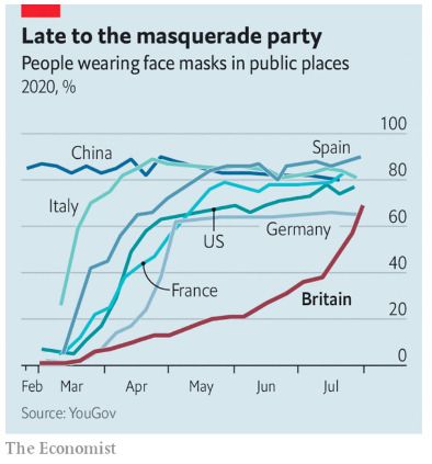
Figure 8: Google Activity: International Evidence
20
Percent change relative to baseline
0
Germany
-20
-40 Italy U.S.
-60 U.K.
-80 Spain
-100
Feb Mar Apr May Jun Jul Aug Sep
2020
Note: Google activity is the equally-weighted average of the “retail and entertainment” and
“workplace” categories. The data are smoothed with an HP filter with smoothing parameter 400.
4.1 Google Activity over Time
Figures 8 shows the (smoothed) Google activity data over time for a large number of
countries, highlighting a few. Italy and Spain show very sharp declines in activity start-
ing quite early compared to the declines in the U.S., the U.K., and Germany. Activity re-
covers somewhat in May in Italy and Spain, but only gradually in the U.K. This appears
to be a case of the U.K. being slow to get the pandemic under control, suffering from
more deaths as a result, and being forced to keep its economy shut down for longer.
The U.S. and Germany are also interesting, in comparison. They have somewhat
similar changes in activity, but, as we’ve seen, very different COVID outcomes. Among
the highlighted countries, Germany had the smallest loss in economic activity and the
fewest deaths.
Next, consider Figure 9 which highlights the Scandinavian countries. These coun-
tries have even milder shutdowns than Germany and the United States. Sweden’s shut-
down is initially the mildest but by the end of June it trails Germany, Denmark, and
Norway slightly.MACROECONOMIC OUTCOMES AND COVID-19 19
Figure 9: Google Activity: Northern Europe
20
Percent change relative to baseline
0
Denmark
Sweden
-20
Norway
U.S.
-40
Germany
-60
-80 Spain
-100
Feb Mar Apr May Jun Jul Aug Sep
2020
Note: Google activity is the equally-weighted average of the “retail and entertainment” and
“workplace” categories. The data are smoothed with an HP filter with smoothing parameter 400.
Global Cities. Figure 10 shows the Google activity measure for 14 key international
cities or regions. Lombardy and Seoul have very early shutdowns with 20 percent de-
clines in activity by the first of March. Madrid and Paris and then New York City and fi-
nally London follow them down, with all four seeing activity down by around 80 percent
as of April 1. Seoul recovers very quickly, while Tokyo sees a slow decline. Stockholm
also has mild losses according to the Google activity measure.
U.S. States. Figure 11 shows the Google activity data for U.S. states. The heterogeneity
of experience stands out, with some states close to “normal” by early August while
others are 30 to 40 percent below baseline. Interestingly, Washington DC stands out:
it has the largest decline of any state at virtually all dates, with activity more than 50
percent below baseline even as of mid August. Recall the contrast with the unemploy-
ment data shown earlier in Figures 6 and 7. As the nation’s capital, Washington DC is
a special place: a large fraction of jobs are in the government sector and so therefore
experienced small declines, while many employees are highly mobile, both nationally
and internationally, resulting in large losses in Google activity.20 FERNÁNDEZ-VILLAVERDE AND JONES
Figure 10: Google Activity for Key Global Cities
20
Percent change relative to baseline
0
Seoul
Stockholm
-20 Tokyo
-40 Lombardy
London
-60
NYC
-80 Madrid
Paris
-100
Feb Mar Apr May Jun Jul Aug Sep
2020
Note: Google activity is the equally-weighted average of the “retail and entertainment” and
“workplace” categories. The data are smoothed with an HP filter with smoothing parameter 400.
Figure 11: Google Activity for Key U.S. States
20
Percent change relative to baseline
0
Texas
-20
Florida
Arizona
-40 California
New York D.C.
-60
-80
Feb Mar Apr May Jun Jul Aug Sep
2020
Note: Google activity is the equally-weighted average of the “retail and entertainment” and
“workplace” categories. The data are smoothed with an HP filter with smoothing parameter 400.MACROECONOMIC OUTCOMES AND COVID-19 21
Figure 12: Google Activity for Key U.S. States and Countries
20
Percent change relative to baseline
0
Germany
-20
Florida
New York California
-40 Italy
-60 U.K.
-80
Feb Mar Apr May Jun Jul Aug Sep
2020
Note: Google activity is the equally-weighted average of the “retail and entertainment” and
“workplace” categories. The data are smoothed with an HP filter with smoothing parameter 400.
Finally, Figure 12 combines some of the key states and countries into a single graph
for ease of comparison. The declines in Google activity in Italy and the U.K. are sub-
stantially larger than the declines in New York state and California, while Germany
stands out as having even milder declines in activity than Florida. While the U.K. was
slower than Italy (and slower than Spain and Germany — see Figure 8) to shut down, it
was as fast as New York and contracted economic activity more severely. New York state
had much worse outcomes in terms of deaths (1700 versus 700), and this is true even if
we compare New York City (2800) versus London (650)22 FERNÁNDEZ-VILLAVERDE AND JONES
4.2 Correlating Economic Activity and Google Mobility
Figure 13: Cumulative Google Activity and Lost GDP
GDP LOSS (PERCENT YEARS)
7 Spain
OLS Slope = 0.230
France U.K. India
6 Std. Err. = 0.041
R2 = 0.53 Italy
Portugal
5 Mexico
Slovakia Belgium
Estonia
4 Hungary Greece Austria
Czechia Singapore
Germany
Finland
3 Denmark U.S. Israel
Poland
Japan Indonesia
2 Sweden Norway Chile
Korea, South
1
0
Taiwan
-1
0 5 10 15 20 25
GOOGLE CUMULATIVE REDUCED ACTIVITY
Note: “GDP Loss” reports the cumulative loss in GDP since the start of 2020 as a percent of annual GDP.
“Google Cumulative Reduced Activity” measures the total amount of lost Google activity at an annual rate.
The correlation in the graph is 0.73.
Before showing the “tradeoff” graphs with the Google activity measure, we first
demonstrate that this measure is correlated with the GDP loss and cumulative excess
unemployment. The correlation with the GDP loss is shown in Figure 13. Here and
in what follows, we add up the areas in the Google activity graphs shown above to
get a cumulative loss in Google activity. In particular, “Google Cumulative Reduced
Activity” measures the total amount of lost Google activity at an annual rate. A value
of 20 indicates that, relative to baseline, it is as if activity at retail, entertainment, and
workplace locations was reduced by 20 percent for an entire year. For example, a 40
percent reduction in activity each month for six months would deliver this value.
Figure 13 illustrates that the Google activity measure is a useful proxy for economic
activity. The correlation between the loss in GDP and the cumulative reduction in
activity is 0.73 (the square root of 0.54).
Figure 14 shows this same kind of evidence for U.S. states, only this time for cumu-MACROECONOMIC OUTCOMES AND COVID-19 23
Figure 14: Cumulative Google Activity and Cumulative Unemployment
CUMULATIVE EXCESS UNEMPLOYMENT (PERCENT YEARS)
7 NV
OLS Slope = 0.171
Std. Err. = 0.041
6 HI R2 = 0.26
MA
5 MI NY
NJ
CA
RI IL
4 PA FL
NH DE ORVT WA
IN OH
SC
TN CO
3 WV TX
AK AL LA
NCNM VAAZ
OK GA
MS ME WI
IA CT
ND
AR KS MN MD
2 SD MTID MO
KY UT
WY DC
NE
1
6 8 10 12 14 16 18 20 22 24 26
GOOGLE CUMULATIVE REDUCED ACTIVITY (PERCENT YEARS)
Note: The correlation is 0.51; it rises to 0.71 if Washington DC is dropped.
late excess unemployment. The correlation with Google activity is 0.51 if Washington
DC is included, but the “outlier” nature of the District of Columbia has already been
mentioned. The correlation rises to 0.71 if this outlier is dropped.24 FERNÁNDEZ-VILLAVERDE AND JONES
Figure 15: Covid Deaths (Latest) and Cumulative Google Activity (August)
CUMULATIVE REDUCED ACTIVITY(PERCENT YEARS)
25
India
United Kingdom
Spain
20
France Italy
Portugal Belgium
Mexico
15 Austria Switzerland
United States
Indonesia Germany
Norway
10
Japan Denmark Sweden
5 Korea, South
Taiwan
0
0 100 200 300 400 500 600 700 800 900
COVID DEATHS PER MILLION PEOPLE
Note: Google activity is the equally-weighted average of the “retail and entertainment” and
“workplace” categories. “Cumulative” refers to the fact that we add up the losses for every month
since February 2020.
4.3 Cumulative Results
Countries. Figure 15 shows the cumulative lost activity according to the Google mo-
bility data as of August 15. The first thing to appreciate is that the graph looks very
similar to the GDP loss graph in Figure 5. This is of course just another way of saying
that the GDP data and Google data are highly correlated.
The key takeaways from this figure are therefore also similar. Belgium, the U.K.,
Spain, and Italy have both very high deaths and very large losses in macroeconomic
activity. Taiwan, Korea, and Japan, as well as Denmark, Norway, and Germany are in the
lower left of the graph, with good performance on both dimensions. Sweden stands out.
It looks successful compared to countries like the U.K., Spain, and Italy, with similar
deaths but much smaller losses in GDP. On the other hand, compared to Norway and
Germany, Sweden looks much less successful, with similar losses in economic activity
but far more deaths. The United States is a similar case in that it has fewer deaths
and smaller losses in economic activity than the U.K., Spain, and Italy, but looks much
worse than Norway and Germany. India stands out in the “northwest” quadrant of theMACROECONOMIC OUTCOMES AND COVID-19 25
Figure 16: Global Cities: Covid Deaths and Cumulative Google Activity
CUMULATIVE REDUCED ACTIVITY(PERCENT YEARS)
35
New York City
30 SF Bay Area
Paris
London
Madrid, Spain
25
Boston Lombardy, Italy
20
Los Angeles
Miami
Tokyo, Japan Chicago
15
Houston
Stockholm
10
Seoul, Korea
5
0 500 1000 1500 2000 2500 3000
COVID DEATHS PER MILLION PEOPLE
Note:
graph, having large losses in economic activity with comparatively few deaths. The
U.S. and India have the additional disadvantage — discussed more below — that their
situations are still very much evolving.
Cities. Figure 16 shows one of advantages of the Google data by disaggregating to the
city level for a collection of key cities around the world. Broadly speaking, we see the
same types of outcomes for cities that we saw for countries and states with the earlier
macroeconomic data. New York City has by far the highest death rate in the world
at around 2800 per million people. Interestingly, it also has the largest cumulative
economic loss, equivalent to around 32 percent of a year’s activity.
The economic loss is only slightly larger than losses in other cities such as London,
Paris, and San Francisco. These cities have far fewer deaths than New York City, how-
ever, at around 600 per million for London and Paris and just 150 for the San Francisco
Bay Area.
Madrid, Boston, and Lombardy stand out the way Spain and Italy did before, with a
high death rate and large economic losses. In contrast, Seoul and Tokyo are much like
South Korea and Japan. Stockholm also plays the same role that Sweden did.26 FERNÁNDEZ-VILLAVERDE AND JONES
Figure 17: U.S. States: Covid Deaths and Cumulative Google Activity
CUMULATIVE EXCESS REDUCED ACTIVITY (PERCENT YEARS)
26
DC
24
22
20
NY
18 HI CA NJ
16 MA
WA NV MD
FL AZ
14 VT VA
CO PA IL MI
OR MN TX CT
12 RI UT NC NM
WI GA DE LA
KY OH
KS TN NH ALINSC
10 ME NE IA
MO
WV OK
NDAR
8 ID
MS
MT
6
WY AK SD
0 200 400 600 800 1000 1200 1400 1600 1800
COVID DEATHS PER MILLION PEOPLE
Note:
Finally, cities such as Los Angeles, Miami, and Chicago lie in the middle, with deaths
somewhat similar to Paris and London, but with noticeably less cumulative loss in
economic activity.
U.S. States. Figure 17 shows the Google activity data and deaths for U.S. states. Apart
from Washington D.C. — where the large decline in activity contrasts with the small rise
in the unemployment rate, as noted above —the pattern is quite similar to what we saw
in the unemployment data back in Figure 7.MACROECONOMIC OUTCOMES AND COVID-19 27
5. Dynamic Versions of the Trade-off Graphs
We now take advantage of the high-frequency nature of both the Google activity data
and the Covid data to examine the dynamic evolution of our outcomes. In what fol-
lows, we show our outcomes at the monthly frequency, from March through the latest
available data (currently August 15). Each dot in the graph is a monthly observation,
connected in order, and with the location name highlighted next to the most recent
observation. After experimenting with different ways of showing these data, we focus
on plots for the current (flow) Google activity measure instead of the cumulative loss in
economic activity.9
Figure 18: Monthly Evolution from March to August
REDUCED ACTIVITY (PERCENT)
80
70
60
50
40
30 United Kingdom
United States
20
Italy
Norway Germany Sweden
10
0
1 2 4 8 16 32 64 128 256 512 1024 2048
COVID DEATHS PER MILLION PEOPLE
Note: Omits February to make more readable. log(1+deaths), deaths from the 15th of each month.
Countries. Figure 18 shows the dynamics for the flow of Google activity for a small
set of countries, focused on the U.S. and some key European economies. The general
pattern is that between March and April, countries move sharply up and to the right,
as Covid deaths explode and the economies severely restrict economic activity. After
April, countries break in two directions. Italy, Germany, Norway, and the U.K. see their
9
These latter graphs with cumulative activity are shown in Appendix B.3.28 FERNÁNDEZ-VILLAVERDE AND JONES
Covid deaths stabilize either by May or certainly by June, and economic activity starts
to recover: the dynamics take the lines sharply downward. In Sweden and the United
States, in contrast, the pandemic continues: deaths continue to increase and economic
activity recovers much less; the movement is more to the right instead of straight down.
Figure 19 shows this same kind of graph for an additional dozen countries including
Taiwan, South Korea, India, Japan, Mexico, France, and Spain. The same two types of
experiences are seen among these additional countries. Most have a large sharp move
up and to the right followed by a recovery in economic activity and a stabilization of
deaths, illustrated by the vertical nature of the lines in the graph. In contrast, Mexico,
India, and Indonesia experience a persistent move to the right as the pandemic contin-
ues and deaths have yet to stabilize.
Figure 19: Monthly Evolution from March to August
REDUCED ACTIVITY (PERCENT)
80
70
60
50
India
40
30 Mexico
Belgium
Spain
20 France
Switzerland
Japan Indonesia Austria Portugal
10 Korea, South
Taiwan Denmark
0
1 2 4 8 16 32 64 128 256 512 1024 2048
COVID DEATHS PER MILLION PEOPLE
Note: Omits February to make more readable. log(1+deaths), deaths from the 15th of each month.
Global cities. Figure 20 shows similar dynamics for key cities around the world. New
York City, Lombardy, Madrid, London, and Paris all move sharply up and to the right
with the onset of the pandemic. By May, however, the stabilization of deaths and the
gradual reopening of the economies is apparent in the vertical portion of the curve.
Stockholm is an interesting contrast in that Google activity declines by only aboutMACROECONOMIC OUTCOMES AND COVID-19 29
Figure 20: Global Cities: Monthly Evolution from March to August
REDUCED ACTIVITY (PERCENT)
90
80
70
60 New York City
50 Paris
London
40 Madrid, Spain
Lombardy, Italy
30 Tokyo, Japan
Stockholm
20
Seoul, Korea
10
0
1 2 4 8 16 32 64 128 256 512 1024 2048
COVID DEATHS PER MILLION PEOPLE
Note: log(1+deaths), deaths from the 15th of each month.
20 to 30 percent for the entire spring, far less than in many other cities. On the other
hand, the rightward move continues for longer, resulting in appreciably more deaths.
Finally, Tokyo and Seoul are interesting to compare. Tokyo had a much larger de-
cline in economic activity peaking at around 45 percent in April and May. By compari-
son, Seoul saw reductions of 15 percent or less each month. While both cities end with
enviably low deaths, the death rate in Seoul is less than 2 per million versus more than
ten times larger at 24 per million in Tokyo.
Figure 21 shows a similar graph for several other cities in the United States. Here
the continued rightward moves in Houston, Miami, Los Angeles, and San Francisco are
evidence that the pandemic is not yet under control.
U.S. states. The next two figures show the dynamics for U.S. states, confirming the
two types of patterns we’ve seen in countries and cities. Figure 22 shows that in states
like New York, New Jersey, Massachusetts, Michigan, and Pennsylvania, deaths have
stabilized. By contrast, Figure 23 shows many states where this is not true.30 FERNÁNDEZ-VILLAVERDE AND JONES
Figure 21: Global Cities: Monthly Evolution from March to August
REDUCED ACTIVITY (PERCENT)
80
70
60
SF Bay Area
50
40 Boston
Los Angeles
Miami
30
Houston Chicago
20
10
1 2 4 8 16 32 64 128 256 512 1024 2048
COVID DEATHS PER MILLION PEOPLE
Note: log(1+deaths), deaths from the 15th of each month.
Figure 22: U.S. States: Monthly Evolution from April to August
REDUCED ACTIVITY (PERCENT)
65
60
55
50
DC
45
40
35
CA
30
NY
25 WA MA NJ
20 PA
MI
15
1 2 4 8 16 32 64 128 256 512 1024 2048
COVID DEATHS PER MILLION PEOPLE
Note: Omits March to make more readable. log(1+deaths), deaths from the 15th of each month.MACROECONOMIC OUTCOMES AND COVID-19 31
Figure 23: U.S. States: Monthly Evolution from April to August
REDUCED ACTIVITY (PERCENT)
50
40
30 FL AZ
VA TX
GA
20 NC
KY OH
AL
10
MT
0
SD
-10
1 2 4 8 16 32 64 128 256 512 1024 2048
COVID DEATHS PER MILLION PEOPLE
Note: Omits March to make more readable. log(1+deaths), deaths from the 15th of each month.32 FERNÁNDEZ-VILLAVERDE AND JONES
6. Conclusion
We have combined data on GDP, unemployment, and Google’s COVID-19 Community
Mobility Reports with data on deaths from COVID-19 to study the pandemic’s macroe-
conomic outcomes.
Our main finding is that most countries/regions/cities fall in either of two groups:
large GDP losses and high fatality rates (New York City, Lombardy, United Kingdom,..)
or low GDP losses and low fatality rates (Germany, Norway, Kentucky, ...). Only a few
exceptions, mainly California and Sweden, depart from this pattern.
This correlation has a simple explanation at a mechanical level. Either through
government mandates or voluntary changes in behavior, those areas that suffered high
mortality reduced economic activity dramatically to lower social contacts and slow
down the spread of the pandemic.
Also, this observation would suggest that controlling the epidemic is also vital to
mitigate GDP losses. It is easy to be sympathetic with this view, as it seems to avoid the
classical trade-offs in economics between alternative ends. With COVID-19, it might be
possible to do better in terms of GDP and mortality.
At the same time, it is incredibly challenging, given our current data, to tell whether
a low death toll was the product of bad luck or bad policy. South Korea and Germany
have been praised by their early and aggressive testing programs and intensive use of
contact tracing. But South Korea might have been hit by a less contagious form of the
virus, and much of the circulation of SARS-CoV-2 in Germany might have occurred
among younger cohorts than in other European countries.
These arguments also work in reverse when we analyze the two main outliers in our
data set: California and Sweden. California seems to have lost too much GDP given the
severity of the health crisis it faced. Sweden could have reduced its mortality without
too much GDP loss, at least as suggested by its Nordic neighbors’ performance. But
again, California was hit early by the first form of virus, perhaps less contagious. From
the perspective of California’s policymakers, the decisions taken ex ante in March might
be fully justified even if too tight ex post. Sweden’s might have suffered from higher
density in Stockholm and other social differences with its neighbors.
Finally, we should notice that COVID-19 has policy spillovers. Had Italy controlled
its epidemic earlier, France and Germany might have suffered a much milder healthMACROECONOMIC OUTCOMES AND COVID-19 33 crisis. And if China had not undertaken draconian measures in Wuhan, South Korea might look today very differently. Before rushing to judgment, these spillover effects must be analyzed in more detail. Our conclusions are subject to a fundamental caveat. Health professionals in China started to suspect the presence of a new respiratory disease in the last week of Decem- ber 2019. The first public message regarding the pandemic occurred on December 31, 2019, and was reported as a minor news item by a few Western media outlets. Only nine months have passed since that news. Furthermore, the pandemic continues and, even in the best-case scenarios were effective vaccines and fast antigens become widely available by early 2021, we still face, at the very least, several more months of the current situation. All the graphs that we have reported may very well look quite different six months from now. Furthermore, by then, it would be much more transparent how much of the divergence in outcomes was driven by luck or policy.
You can also read