Magnetosheath plasma flow model around Mercury - ANGEO
←
→
Page content transcription
If your browser does not render page correctly, please read the page content below
Ann. Geophys., 39, 563–570, 2021
https://doi.org/10.5194/angeo-39-563-2021
© Author(s) 2021. This work is distributed under
the Creative Commons Attribution 4.0 License.

Magnetosheath plasma flow model around Mercury
Daniel Schmid, Yasuhito Narita, Ferdinand Plaschke, Martin Volwerk, Rumi Nakamura, and Wolfgang Baumjohann
Space Research Institute, Austrian Academy of Sciences, Graz, Austria

Correspondence: Daniel Schmid (daniel.schmid@oeaw.ac.at)

Received: 3 January 2021 – Discussion started: 8 January 2021
Revised: 26 April 2021 – Accepted: 27 April 2021 – Published: 24 June 2021

Abstract. The magnetosheath is defined as the plasma re-        tial equations of an unmagnetized fluid around an obstacle,
gion between the bow shock, where the super-magnetosonic        represented by the magnetosphere. It has successfully been
solar wind plasma is decelerated and heated, and the outer      tested against in situ spacecraft data (Song et al., 1999; Sta-
boundary of the intrinsic planetary magnetic field, the so-     hara et al., 1993; Spreiter and Alksne, 1968) and applied to
called magnetopause. Based on the Soucek–Escoubet mag-          model the magnetospheres of various planets in our solar sys-
netosheath flow model at the Earth, we present an analyti-      tem (see Stahara, 2002, for a review). A decisive drawback
cal magnetosheath plasma flow model around Mercury. The         of this model, however, is the high complexity and computa-
model can be used to estimate the plasma flow magnitude         tional demands to calculate numerically a set of differential
and direction at any given point in the magnetosheath exclu-    equations.
sively on the basis of the plasma parameters of the upstream       To reduce the computational complexity, several analyt-
solar wind. The model serves as a useful tool to trace the      ical plasma flow models have alternatively been proposed
magnetosheath plasma along the streamline both in a forward     (Russell et al., 1983; Kallio and Koskinen, 2000; Romashets
sense (away from the shock) and a backward sense (toward        et al., 2008). An analytical magnetosheath flow model, which
the shock), offering the opportunity of studying the growth     has successfully been tested against spacecraft observations
or damping rate of a particular wave mode or evolution of       at Earth, has been implemented by Soucek and Escoubet
turbulence energy spectra along the streamline in view of up-   (2012). This model is based on the magnetic field model
coming arrival of BepiColombo at Mercury.                       developed by Kobel and Flückiger (1994) and later modi-
                                                                fied and extended by Génot et al. (2011) to obtain a mag-
                                                                netosheath plasma flow model. The essential advantage of
                                                                this model is its compatibility with a wide range of bow
1   Introduction                                                shock and magnetopause models while retaining the sim-
                                                                plicity and computational efficiency of the original magnetic
The magnetosphere of a planet constitutes an obstacle to        field model. Furthermore, the model allows us to calculate
the super-magnetosonic solar wind. Upstream of the planet       the plasma flow velocity at any point in the magnetosheath
a bow shock emerges, because the interplanetary magnetic        using only the spacecraft position and solar wind parameter
field (IMF), embedded in the solar wind, cannot simply          upstream of the bow shock.
penetrate the magnetosphere. At the bow shock the super-           In this work we follow the procedure proposed by Soucek
magnetosonic solar wind plasma is decelerated and heated.       and Escoubet (2012) and rescale their terrestrial magne-
The region with the subsonic, heated plasma downstream of       tosheath flow model to the space environment at Mercury.
the bow shock is called magnetosheath. The magnetosheath        First, we introduce the Hermean bow shock and magne-
plays an important role in the interaction between bow shock    topause model, used to obtain the magnetosheath plasma
and magnetosphere as it conveys energy between the solar        flow model. Second, we revisit the magnetic field model
wind and the planetary magnetosphere.                           of Kobel and Flückiger (1994) which Soucek and Escoubet
   One of the earliest magnetosheath plasma flow models         (2012) used to determine the plasma velocity direction in the
is the hydrodynamic model introduced by Spreiter et al.         magnetosheath. Third, we extend the model by the Rankine–
(1966). Basically the model solves the gas-dynamic differen-

Published by Copernicus Publications on behalf of the European Geosciences Union.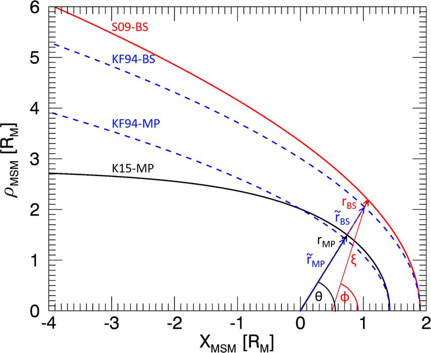
564 D. Schmid et al.: Mercury Streamline Model
Hugoniot relations in a similar way as Génot et al. (2011) to
determine the velocity magnitude downstream of the shock.
The aim of this paper is to provide a tool to estimate the
plasma flow at a given point of spacecraft observation inside
the Hermean magnetosheath on the basis of the solar wind
conditions.
2 Bow shock and magnetopause model at Mercury
In the following we use an aberrated Mercury Solar Mag-
netospheric (MSM) coordinate system. This coordinate sys-
tem is based on the Mercury Solar Orbital (MSO) coordi-
nate system, but its origin is shifted northward by 479 km
from the MSO origin to account for Mercury’s dipole off-
set and rotated into the solar wind velocity direction. In the
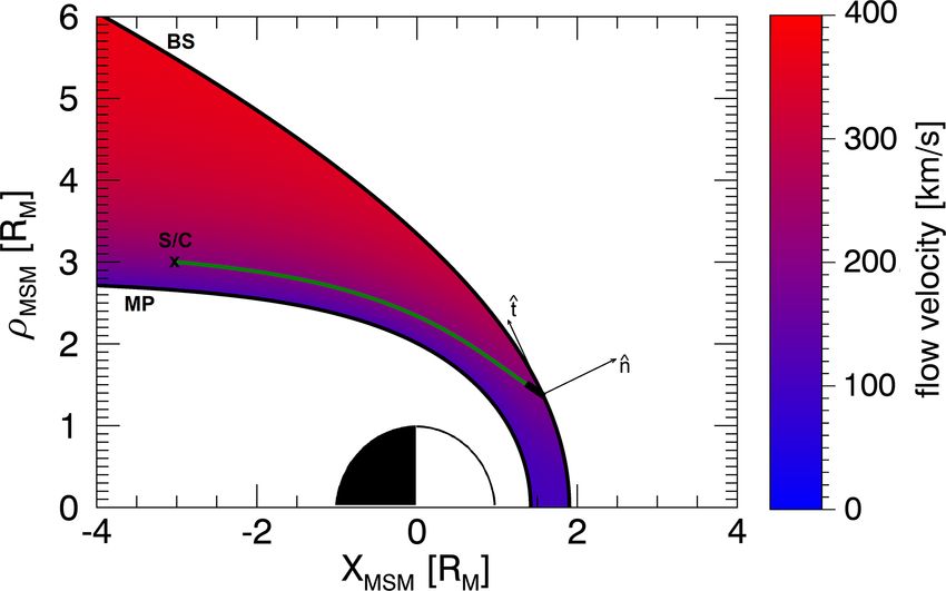
MSO coordinate system the XMSO axis points sunward, the Figure 1. Schematic representation of the parameters used in the
YMSO axis points antiparallel to Mercury’s orbital velocity formulation of the bow shock and magnetopause in the MSM equa-
and ZMSO = XMSO × YMSO completes the right-handed sys- torial plane. The solid red line is the bow shock evaluated from
tem. To compensate for the aberration of the solar wind Eq. (2) (S09-BS; Slavin et al., 2009). The solid black line repre-
direction due to the orbital motion of Mercury around the sents the magnetopause determined by Eq. (3) (K15-MP; Korth
et al., 2015). The dashed blue lines are the bow shock and magne-
sun, the XMSO axis is rotated antiparallel to the solar wind
topause determined by Eq. (4) from the KF94 model (Kobel and
flow velocity direction. In the MSM coordinate system the
Flückiger, 1994).
bow shock and magnetopause models are considered to be
cylindrically symmetric around the XMSM axis, reducing the
three dimensions {XMSM ,qYMSM , ZMSM } to two dimensions Figure 1 shows a schematic illustration of the parameters ξ ,
{XMSM , ρMSM } with ρ = YMSM 2 2
+ ZMSM . φ, rBS and θ , which are used in the formulation of the bow
Slavin et al. (2009) modeled the bow shock at Mercury by shock.
a conic section of the form Korth et al. (2015) used the magnetopause model proposed
q
p from Shue et al. (1997) and found that the MESSENGER
ξ = (xBS − x0 )2 + ρBS 2 = , (1) observations of magnetopause crossing are best fit by
1 + cos φ
α
2
q
with x0 being the distance of the focus of theqconic sec- rMP = 2 + ρ2
xMP = RMP , (3)
MP
2 + z2 1 + cos θ
tion from the dipole center along XMSM , ρBS = yBS BS
being the distance from the XMSM axis, p being the focal with α = 0.5 being the best-fit flaring parameter, and RMP =
parameter and being the eccentricity. With the advent of 1.42 RM being the subsolar stand-off magnetopause distance.
the MESSENGER (MErcury Surface, Space ENvironment, Figure 1 shows the Slavin et al. (2009) bow shock model
GEophysics and Ranging; Solomon et al., 2007) spacecraft (S09-BS) and Korth et al. (2015) magnetopause model (K15-
in an orbit around Mercury, it was possible to characterize MP) evaluated from Eqs. (2) and (3), respectively.
the spatial location of the bow shock and magnetopause sta-
tistically. Winslow et al. (2013) determined that the best-fit
parameters to the bow shock are given by x0 = 0.5 RM , p = 3 The KF94 magnetic field model
2.75 RM and = 1.04. With these parameters the extrapo-
lated subsolar bow shock stand-off distance is RBS = 1.9 RM To obtain the magnetosheath plasma flow direction, we fol-
(Mercury radii, 1 RM ∼ 2440 km). For this work, it is advan- low the procedure proposed by Soucek and Escoubet (2012)
tageous to transform Eq. (1) into the origin of the MSM co- and use the magnetic field model developed by Kobel and
ordinate system with Flückiger (1994). In the following we denote this model
q as KF94 model and mark all quantities pertaining to the
rBS = (ξ cos φ + x0 )2 + (ξ sin φ)2 , KF94 model by a tilde, e.g., r̃. In the KF94 model the bow
shock (BS) and magnetopause (MP) at Mercury are modeled
ξ cos φ + x0
θ = arccos , (2) by parabolic surfaces at a common focus with
rBS
q
where rBS is the distance from the dipole center to the bow − cos θ + cos2 θ + 4R{BS,MP} b{BS,MP} sin2 θ
r̃{BS,MP} = , (4)
shock, and θ is the angle between rBS and the XMSM axis. 2b{BS,MP} sin2 θ
Ann. Geophys., 39, 563–570, 2021 https://doi.org/10.5194/angeo-39-563-2021D. Schmid et al.: Mercury Streamline Model 565
with bBS = 1/(4RBS − 2RMP ) and bMP = 1/(2RMP ) defined 1. As a first
p step, we calculate the angle θ =
by the stand-off distances R{BS,MP} . arccos(x/ x 2 + ρ 2 ) between r and the XMSM axis.
Under the assumption that the IMF is parallel to the solar
wind, the magnetic field lines of the KF94 model represent 2. Then we estimate the fractional distance, F, of r be-
the flow lines of the solar wind and magnetosheath plasma. tween the bow shock and magnetopause from Eqs. (2)
Using the magnetic field vector direction in the KF94 model, and (3) with
Soucek and Escoubet (2012) determined the flow velocity r(θ ) − rBS (θ )
vector at a given position r = (x, ρ) by F= . (9)
rBS (θ ) − rMP (θ )
ṽx = vm (C/2d − C/RMP ),
3. Now we change into the KF94 model and calculate
ṽρ = vm (Cρ/[2d(d + x − RMP /2)]), (5) r̃BS (θ ) and r̃MP (θ ) from Eq. (4) with the angle θ . Note
that the stand-off distances (RBS and RMP ) and the fo-
where vm corresponds to the flow velocity magnitude, d = cus (r 0 = (RMP /2, 0)) in Eq. (4) are the best-fit values
|r − r 0 | is the difference between the given position in from Eqs. (2) and (3).
the magnetosheath and the parabolic surface focus r 0 =
(RMP /2, 0) and C = RMP (2RBS −RMP )/(2RBS −2RMP ) is a 4. In a next step we determine the fractional position
constant defined by the bow shock and magnetopause stand- within the magnetosheath in the KF94 model with
off distances.
r̃(θ ) = F[r̃BS (θ ) − r̃MP (θ )] + r̃BS (θ ), (10)
4 The magnetosheath plasma flow model around according to Eq. (9).
Mercury 5. Using Eq. (5) we evaluate the KF94 flow velocity vec-
tor, ṽ for ṽ = (ṽx , ṽρ ) at the position r̃(θ ). Note that the
To obtain the magnetosheath plasma flow at a specific point velocity magnitude vm is determined in a later step.
(r = (x, ρ)) in the magnetosheath at Mercury, we evaluate
the plasma flow direction first and then determine the magni- 6. With the obtained flow velocity vector, v, we are able to
tude of the velocity vector from the Rankine–Hugoniot rela- estimate the new position of an adjacent point along the
tion across the bow shock. same flow line r̃ 0 = r̃ + ṽ1t, by choosing an infinitesi-
A magnetic field model is used to describe the plasma flow mally small time increment 1t.
here. The reason for this is explained as follows. Assump-
tions are made such that there are no proton sinks or sources 7. Next we determine the angle between the new position
in the magnetosheath. Strictly speaking, this assumption is and the XMSM axis, θ 0 , and the fractional distance inside
only weakly justified because of the neutral particles such as the KF94 magnetosheath, F 0 , using Eq. (9).
the hydrogen corona and the sodium exosphere around Mer- 8. Finally we transform the new position r̃ 0 (θ 0 ) back from
cury. A stationary case is taken in the fluid picture. The con- the KF94 model to the original MSM reference frame
tinuity equation reads then as where the magnetosheath is confined by Eqs. (2) and
(3). The new position, r 0 , inside this magnetosheath is
∇ · (nU ) = 0, (6)
then given by
where n and U are the density and velocity of protons, re- r 0 = F 0 [r BS (θ 0 ) − r MP (θ 0 )] + r BS (θ 0 ), (11)
spectively. Now we make an analogy such that
and thus the plasma flow direction can be determined by
(nU ) −→ B, (7) v = (r 0 − r)/1t.
holds, and Eq. (6) is equivalent to the divergence-free condi- Applying recursively this procedure (steps 1–8) yields the
tion of magnetic field: plasma flow line within Mercury’s magnetosheath. In Fig. 2
five examples of flow lines are shown.
∇ · B = 0. (8)
4.2 Plasma flow magnitude
For a more detailed discussion, see e.g., Génot et al. (2011).
To evaluate the magnetosheath plasma velocity magnitude,
4.1 Plasma flow direction vm , we apply the Rankine–Hugoniot (RH) equations, which
relate the upstream (u) with the downstream (d) plasma con-
Following the procedure proposed by Soucek and Escou- ditions. The downstream plasma flow velocity directly be-
bet (2012), we rescale the plasma flow direction from the hind the bow shock, v d , is derived by the following proce-
KF94 model to Mercury’s space environment as follows: dure:
https://doi.org/10.5194/angeo-39-563-2021 Ann. Geophys., 39, 563–570, 2021566 D. Schmid et al.: Mercury Streamline Model
sion ratio between the upstream and downstream mass
density, θVn = arctan(vtu /vnu ) is the angle between the
upstream velocity vector and the shock normal, θBn =
arctan(Btu /Bnu ) is the angle between upstream magnetic
√ u
field vector and shock normal, and MAu = vnu µB0uρ is
n
the upstream Alfvén Mach number.
4. In Eq. (13) all parameters pertain to the upstream side,
except the compression ratio R. However, R can also
be expressed by exclusively upstream parameters with
(see e.g., Anderson, 1963)
(MAu 2 − R)2 (γ β u R + MAu 2 cos2 θBn [(γ − 1)
R − (γ + 1)]) + RMAu 2 sin2 θBn ([γ + (2 − γ )R]
Figure 2. Schematic representation of the flow lines (red) in the MAu 2 + R[(γ − 1)R − (γ + 1)]) = 0 (14)
MSM equatorial plane. The solid black lines are the bow shock and
magnetopause evaluated from Eqs. (2) and (3), respectively. where β u = (2µ0 p u )/B u 2 is the ratio of the upstream
thermal to magnetic pressures, and γ is the polytropic
index which is typically assumed to be γ = 5/3. Equa-
1. From the given spacecraft position in the magne- tion (14) is equivalent to Eq. (2.43) in Anderson (1963)
tosheath, r = (x, ρ), we trace the flow line back to the with different notations. The solution is given in the
bow shock. Thereto we iteratively apply steps (1)–(8) form of compression ratio as a function of the shock
from above, with reversed increments r̃ 0 = r̃ − ṽ1t in angle θBn . Solutions exist for a compression ratio in the
step (6), until the bow shock is reached (F 0 = 0). Then range 1 ≤ R ≤ 4 when using Eq. (14). Another class of
we calculate the angle θBS between the XMSM axis and solutions also exists for the expansion (R < 1) with a
the bow shockq intersection at (xBS , ρBS ) with θBS = decrease of entropy from the upstream onto the down-
2 + ρ 2 ).
arccos(xBS / xBS stream side. The latter case is not physically relevant
BS
and is not considered here. The upper limit of com-
2. In a next step we determine the bow shock tangent t̂ and pression ratio (R = 4) corresponds to the limit of high
normal n̂ unit vectors where the back-traced flow line Alfvén Mach number (MA → ∞) under a polytropic in-
intersects the bow shock. For any point along the bow dex of γ = 5/3.
shock, the normal, n, and tangent, t, vector can easily
5. By solving Eq. q(14) for R the downstream velocity
be computed by 2
2
magnitude vd = vnd + vtd is therefore entirely deter-
drBS drBS
t=
dθ
cos θ − rBS sin θ êx +
dθ
sin θ + rBS cos θ êρ , mined by only the upstream plasma parameters.
drBS drBS Since the detailed density profile along the flow line is
n= sin θ + rBS cos θ êx − cos θ + rBS sin θ êρ , (12)
dθ dθ
unknown, we assume in a first approximation a constant
where drdθBS is numerically calculated from two consec- plasma density and thus a constant velocity magnitude along
utive points along the bow shock given by Eq. (2). The the flow line. Therefore, the velocity magnitude at a given
shock frame of reference is then defined by the normal- point r directly corresponds to the velocity magnitude down-
ized normal and tangent vector at θBS . stream of the shock, and vm = vd . Although this assumption
has the tendency to underestimate the velocity close to the
3. In the shock reference frame the RH equations can be magnetopause, it yields satisfactory results in a first approach
combined to determine the downstream velocity vector (Génot et al., 2011).
component parallel v dn and perpendicular v dt to the shock The entire procedure from above is implemented in an
normal (see e.g., Génot, 2008): IDL computer program which can be retrieved from OSF
1 (Schmid, 2020). The program is designed to evaluate the
v dn = v un , plasma flow velocity vector at a given observation point of
R
a spacecraft inside the Hermean magnetosheath exclusively
1 − 1/R on the basis of the upstream solar wind conditions. As the so-
v dt = v un tan θVn + h i tan θBn , (13)
MAu 2 /(Rcos2 θBn ) − 1 lar wind input parameters, we use the solar wind propagation
model of Tao et al. (2005), which is modified by the orbital
where v un is the upstream velocity vector component motion of Mercury. The model is a one-dimensional magne-
parallel to the shock normal, R = ρ d /ρ u is the compres- tohydrodynamic model and takes the OMNI dataset as input
Ann. Geophys., 39, 563–570, 2021 https://doi.org/10.5194/angeo-39-563-2021D. Schmid et al.: Mercury Streamline Model 567
to compute propagation at all solar system bodies including
Mercury. The correction for the orbital motion is achieved
by adding the solar wind velocity vector, V SW , (which is
radially away from the Sun) and the orbital motion veloc-
ity vector of Mercury, V mercury , with V = V SW + V mercury .
To obtain V mercury , we use the dataset provided from the
Navigation and Ancillary Information Facility (NAIF; Ac-
ton, 1996), which provide the distance between Mercury and
Sun, D, and absolute velocity of Mercury, Vmercury . To deter-
mine aberration velocity vector, we first calculate the aberra-
tion angle φ on the basis of Mercury’s elliptical orbit with
p
φ = arctan b/ a 2 − b2 sin arccos((1 − p/D)/e) , (15)
Figure 3. Color-coded flow speed calculated from Eq. (13) with the
where a is the semimajor axis, b the semiminor axis,
averaged upstream parameters from the Tao et al. (2005) solar wind
p the semi-latus rectum and e the eccentricity of the propagation model at Mercury between 2011 and 2015. Also plotted
ellipse. With the aberration angle φ and the consid- is a schematic representation of back-traced flow line (green) from
eration whether Mercury moves towards or away from a virtual spacecraft (S/C) to the bow shock (BS) with the respective
the sun, we subsequently obtain the aberration veloc- shock normal n̂ and tangent t̂ obtained from Eq. (12). The thick
ity vector V mercury,x = ±Vmercury sin(φ) and V mercury,y = black line downstream of the BS is the downstream velocity vector
±Vmercury cos(φ). The transformation due to this abberation direction determined by Eq. (13). Alfvén Mach number is 5.8, and
effect is made by applying a two-dimensional rotation matrix plasma beta is 0.79.
to the spatial coordinates (spanning the x and ρ coordinates):
0
x cos θa − sin θa x
= , (16) shock normal n̂ and tangent t̂ are illustrated in thin black
y0 sin θa cos θa ρ
lines. The thick black line downstream of the bow shock
where the aberration angle θa is given by the radial solar wind shows the velocity vector direction evaluated from the RH
velocity, V SW , and the apparent solar wind velocity, V with relations, which is in good agreement with the streamline di-
θa = arccos (V SW · V ). In Fig. 3 the results of the model are rection determined by the KF94 model.
shown for the average solar wind plasma parameters during At the virtual spacecraft position the model predicts a
the entire MESSENGER operation service between 2011 and magnetosheath plasma flow velocity of vx ≈ −200 km/s and
2015. After modifying the solar wind velocity vector of the vρ ≈ 17 km/s.
Tao et al. (2005) model by the orbital motion of Mercury A naive picture of the compression by a factor of 4 (in
(Acton, 1996), the average input solar wind plasma param- the limit of high Mach number) is not realistic, because
eters for our model are density of nu ≈ 40 cm−3 , tempera- the interplanetary magnetic field around Mercury reaches a
ture of T ≈ 18 eV, flow speed of |V u | ≈ −400 km/s, mag- magnitude of 20 to 50 nT, and the Alfvén Mach number is
netic field magnitude of |B u | ≈ 20 nT with the radial com- correspondingly smaller than that around the Earth by 20
ponent Br ≈ 18 nT (ignoring the sign) and the tangential to 50, respectively. A picture of the constant density and a
component Bt ≈ 16 nT (ignoring the sign). The mean val- reduced flow speed to 1/4 of the solar wind speed at the
ues of density, temperature, flow speed and magnetic field magnetopause (along the streamline tangential to the mag-
are valid for nearly 1500 d of observations of MESSEN- netopause) is not valid, either, since the adiabatic expansion
GER (confirmed by one of the reviewers). It is worthwhile breaks down, and the model is not applicable to the flow in
to note that one finds an angle of 23◦ from the Tao dataset, the subsolar region and at the magnetopause.
which is consistent to the spiral angle at Mercury at an av-
erage position of 0.4 astronomical units (AU) from the Sun
for a solar wind speed of 400 km/s. The Bx component is 5 Discussion and conclusions
computed from the By component using the Parker spiral
field in the Tao model. The Alfvén Mach number in the up- Here we present the first analytical magnetosheath plasma
stream region is MA = v u /VA ≈ 5.8 (with an Alfvén speed flow model for the space environment around Mercury. The
of VA ≈ 69 km/s), and the plasma parameter beta (upstream) model is based on the magnetosheath model by Soucek and
is β = 2µ0 nkB T /B 2 ≈ 0.72 (where µ0 is the permeability Escoubet (2012), which has successfully been tested against
of free space, and kB is the Boltzmann constant) in our spacecraft observations at Earth. The proposed model is rel-
setup. Color coded is the obtained velocity magnitude vm . atively simple to implement and provides the possibility to
Additionally, the back-traced flow line from a virtual space- trace the flow lines inside the Hermean magnetosheath.
craft located at xMSM = −3 RM and ρMSM = 3 RM is plot- The model presented in this paper is generally robust and
ted (green line). At the bow shock intersection the calculated easy to implement for its analytic expression using upstream
https://doi.org/10.5194/angeo-39-563-2021 Ann. Geophys., 39, 563–570, 2021568 D. Schmid et al.: Mercury Streamline Model parameters. It can help to determine the local plasma con- along the flow line and to test under which conditions the ditions of a spacecraft in the magnetosheath exclusively on adiabatic expansion breaks down. the basis of the upstream solar wind parameters. Two appli- Although the proposed model has a good performance cations are in mind in view of the BepiColombo mission, overall for a wide range of upstream conditions, the accu- where the Mercury Magnetospheric Orbiter (MMO also re- racy strongly depends on the used bow shock and magne- ferred to as Mio) will probe Mercury’s magnetosheath and topause model. Here we utilize the bow shock and magne- solar wind with unprecedented fast measurements of the par- topause model from Slavin et al. (2009) and Korth et al. ticle distribution functions: (1) the Tátrallyay method to ob- (2015), which were adopted from MESSENGER boundary servationally determine the growth rate or damping rate of crossing observations. specific mode such as the mirror mode along the stream- The presented model is cylindrically symmetric around the line (Tátrallyay and Erdös, 2002; Tátrallyay et al., 2008) and XMSM axis. In reality, however, non-radial IMF conditions (2) the Guicking method to observationally track the spec- will lead to a spatially asymmetric magnetosheath (Nishino tral evolution of turbulent fluctuations along the streamline et al., 2008; Dimmock and Nykyri, 2013; Dimmock et al., (Guicking et al., 2010, 2012). 2016). On the quasi-perpendicular side, where the shock- At the moment a comparison with plasma data is techni- normal angles θBn are greater than 45◦ , the magnetosheath is cally not feasible for our model. Due to the limited particle known to be thicker with larger plasma flow velocities than measurements on board MESSENGER, it is not possible to on the quasi-parallel side, where θBn < 45◦ . Such asymme- obtain the plasma parameters properly in the solar wind and tries cannot be reproduced by the simple model presented magnetosheath, that is, by covering the full velocity distribu- here but should be addressed in future work. tions and to compare with the model velocities. Above all, Furthermore, the method used to determine the flow veloc- the plasma instrument is located behind the heat shield and ity magnitude can possibly be improved. Here we assumed has just a limited field of view. Due to this fact, the major- a constant plasma density and velocity along the flow line ity (thermal core part) of solar wind particles cannot be de- which has the tendency to underestimate the plasma veloc- tected. Comparison with the numerical simulations would be ity in regions with lower densities, e.g., close to the magne- another possibility to test for the model, but a quantitative topause. Génot et al. (2011) proposed a simple ad hoc model comparison remains a challenge for the reason that there are of a plasma density profile which has been implemented large discrepancies in the density and flow velocity among by Soucek and Escoubet (2012). While this ad hoc den- various simulation models on the dayside from the subsolar sity model showed good correspondence with in situ space- point to the northern terminator (Aizawa et al., 2021). craft plasma observation at Earth, the solar wind and mag- An approximation that the magnetic field is more aligned netospheric conditions at other planets can be very differ- with the solar wind flow direction is more justified at Mer- ent (like at Mercury) and thus might give a worse prediction cury than at the Earth because of the Parker spiral nature. (Soucek and Escoubet, 2012). Our model inherits the proper- One of the possible consequences of our assumption is that ties from the Soucek–Escoubet model by scaling the Kobel– the magnetic field magnitude would change or evolve in the Flückinger model of the near-Earth environment: (1) time same sense as that of the plasma (or particle number flux) stationary flow and (2) axially symmetric around the axis of in the magnetosheath. The correlation between the magnetic (apparent) solar wind penetrating the planet. Assumption of field and that of the particle flux in the magnetosheath would time stationary flow may break down when the change in ideally be tested against the plasma and magnetic field data the solar wind state is not negligible. Assumption of the ax- on the arrival of BepiColombo at Mercury. The change in the isymmetric magnetosheath may also break down when the number density can be interpreted as the change in the cross- magnetopause location is not symmetric between the north- sectional area of a flux tube across which the plasma streams. ern and the southern hemisphere (in particular, in the tail re- The change in the flow velocity can then be compared with gion). that from the adiabatic expansion and that from the measure- At this stage we decided not to include an ad hoc den- ment. sity profile, also because it can hardly be tested due to the The following remarks are drawn as scientific message. limited plasma observations around Mercury. The assump- First, Fig. 1 visually demonstrates that different models pre- tion of constant density implies a constant velocity along a dict different shapes of the tail and magnetosheath, which is given flow line. The velocity profile may vary considerably an overlooked issue in the Mercury magnetosphere commu- from that estimated in the earlier models such as the Spre- nity. Second, Fig. 2 shows that the flow lines near the sub- iter model (Spreiter et al., 1966), the Genot model (Génot solar region (Sun-to-planet line if neglecting the planetary et al., 2011), and the Soucek–Escoubet model (Soucek and orbital motion) expand abruptly so that the adiabatic expan- Escoubet, 2012). As mentioned above, the constant density sion may break down. In particular, the adiabatic expansion will likely underestimate the propagation timing in the mag- plays an important role in predicting the flow in the mag- netosheath. In future work such a density profile should be netosheath. Logical continuation of our model construction evaluated and included. would be to evaluate also the density and velocity profile Ann. Geophys., 39, 563–570, 2021 https://doi.org/10.5194/angeo-39-563-2021
D. Schmid et al.: Mercury Streamline Model                                                                                                569

Code availability. An IDL program to evaluate plasma flow                    of solar wind conditions, Adv. Spac. Res., 58, 196–207,
velocity vector in Mercury’s magnetosheath from solar                        https://doi.org/10.1016/j.asr.2015.09.039, 2016.
wind parameters of the Tao solar wind propagation model                   Génot, V.: Mirror and Firehose Instabilities in the Heliosheath, As-
can be retrieved from OSF: https://osf.io/9jgqn/?view_only=                  trophys. J., 687, 119–122, https://doi.org/10.1086/593325, 2008.
2624aca3774c4ba8885dcb21a13e1b08 (last access: 25 May 2021)               Génot, V., Broussillou, L., Budnik, E., Hellinger, P., Trávníček, P.
(Schmid, 2020).                                                              M., Lucek, E., and Dandouras, I.: Timing mirror structures ob-
                                                                             served by Cluster with a magnetosheath flow model, Ann. Geo-
                                                                             phys., 29, 1849–1860, https://doi.org/10.5194/angeo-29-1849-
Data availability. The plasma data of the heliospheric Tao model             2011, 2011.
are open-access data and can be retrieved on the AMDA web-                Guicking, L., Glassmeier, K.-H., Auster, H.-U., Delva, M.,
site (http://amda.cdpp.eu/ (last access: 25 November 2020), Cen-             Motschmann, U., Narita, Y., and Zhang, T. L.: Low-frequency
tre de Données de la Physique des Plasmas (CDPP), 2018) via                  magnetic field fluctuations in Venus’ solar wind interaction re-
the WorkSpace Explorer: DataBase/Solar Wind Propagation Mod-                 gion: Venus Express observations, Ann. Geophys., 28, 951–967,
els/Tao Model/SW Input OMNI (Tao et al., 2005). The orbital mo-              https://doi.org/10.5194/angeo-28-951-2010, 2010.
tion data of Mercury are provided by the Navigation and Ancil-            Guicking, L., Glassmeier, K.-H., Auster, H.-U., Narita, Y., and
lary Information Facility (NAIF) and can be retrieved on the NAIF            Kleindienst, G.: Low-frequency magnetic field fluctuations in
website under https://wgc.jpl.nasa.gov:8443/webgeocalc (last ac-             Earth’s plasma environment observed by THEMIS, Ann. Geo-
cess: 6 May 2020) (Acton, 1996).                                             phys., 30, 1271–1283, https://doi.org/10.5194/angeo-30-1271-
                                                                             2012, 2012.
                                                                          Kallio, E. J. and Koskinen, H. E. J.: A semiempirical mag-
Author contributions. DS initiated this study, collected the data and        netosheath model to analyze the solar wind-magnetosphere
implemented the method. FP, YN, MV and WB helped with evalu-                 interaction, J. Geophys. Res.-Space, 105, 469–479,
ating the article.                                                           https://doi.org/10.1029/2000JA900086, 2000.
                                                                          Kobel, E. and Flückiger, E. O.: A model of the steady state magnetic
                                                                             field in the magnetosheath, J. Geophys. Res.-Space, 99, 617–622,
                                                                             https://doi.org/10.1029/94JA01778, 1994.
Competing interests. The authors declare that they have no conflict
                                                                          Korth, H., Tsyganenko, N. A., Johnson, C. L., Philpott, L. C.,
of interest.
                                                                             Anderson, B. J., Al Asad, M. M., Solomon, S. C., and
                                                                             McNutt Jr., R. L.: Modular model for mercury’s magne-
                                                                             tospheric magnetic field confined within the average ob-
Financial support. This research has been supported by the Öster-            served magnetopause, J. Geophys. Res.-Space, 120, 4503–4518,
reichische Forschungsförderungsgesellschaft (grant no. 865967).              https://doi.org/10.1002/2015JA021022, 2015.
                                                                          Nishino, M. N., Fujimoto, M., Phan, T.-D., Mukai, T.,
                                                                             Saito, Y., Kuznetsova, M. M., and Rastätter, L.: Anoma-
Review statement. This paper was edited by Anna Milillo and re-              lous Flow Deflection at Earth’s Low-Alfvén-Mach-
viewed by two anonymous referees.                                            Number Bow Shock, Phys. Res. Lett., 101, 065003,
                                                                             https://doi.org/10.1103/PhysRevLett.101.065003, 2008.
                                                                          Romashets, E. P., Poedts, S., and Vandas, M.: Modeling of the mag-
                                                                             netic field in the magnetosheath region, J. Geophys. Res.-Space,
References                                                                   113, A2, https://doi.org/10.1029/2006JA012072, 2008.
                                                                          Russell, C. T., Luhmann, J. G., Odera, T. J., and Stuart, W. F.: The
Acton, C. H.: Ancillary data services of NASA’s Navigation and               rate of occurrence of dayside Pc 3,4 pulsations: The L-value de-
  Ancillary Information Facility, Planet. Space Sci., 44, 65–70,             pendence of the IMF cone angle effect, Geophys. Res. Lett., 10,
  https://doi.org/10.1016/0032-0633(95)00107-7, 1996.                        663–666, https://doi.org/10.1029/GL010i008p00663, 1983.
Anderson, J. E.: Magnetohydrodynamic shock waves, Cambridge:              Schmid, D.: Mercury Streamline Model: IDL code, OSF, available
  MIT Press, 1963.                                                           at: https://osf.io/9jgqn (last access: 25 May 2021), 2020.
Aizawa, S., Griton, L. S., Fatemi, S., Exner, W., Deca, J., Pantellini,   Shue, J.-H., Chao, J. K., Fu, H. C., Russell, C. T., Song,
  F., Yagi, M., Heyner, D., Génot, V., André, N., Amaya, J., Mu-             P., Khurana, K. K., and Singer,H. J.: A new functional
  rakami, G., Beigbeder, L., Gangloff, M., Bouchemit, M., Budnik,            form to study the solar wind control of the magnetopause
  E., and Usui, H.: Cross-comparison of global simulation models             size and shape, J. Geophys. Res.-Space, 102, 9497–9511,
  applied to Mercury’s dayside magnetosphere, Planet. Space Sci.,            https://doi.org/10.1029/97JA00196, 1997.
  198, 105176, https://doi.org/10.1016/j.pss.2021.105176, 2021.           Slavin, J. A., Anderson, B. J., Zurbuchen, T. H., Baker, D. N.,
Dimmock, A. P. and Nykyri,K.: The Statistical Mapping of                     Krimigis, S. M., Acuña, M. H., Benna, M., Boardsen, S. A.,
  Magnetosheath Plasma Properties Based on THEMIS Mea-                       Gloeckler, G., Gold, R. E., Ho, G. C., Korth, H., McNutt Jr.,
  surements in the Magnetosheath Interplanetary Medium Ref-                  R. L., Raines, J. M., Sarantos, M., Schriver, D., Solomon, S. C.,
  erence Frame, J. Geophys. Res.-Space, 118, 4963–4976,                      and Trávnícek, P.: Messenger observations of Mercury’s mag-
  https://doi.org/10.1002/jgra.50465, 2013.                                  netosphere during northward IMF, Geophys. Res. Lett., 36, 2,
Dimmock, A. P., Nykyri, K., Osmane, A., and Pulkkinen,                       https://doi.org/10.1029/2008GL036158, 2009.
  T. I.: Statistical mapping of ULF Pc3 velocity fluctua-
  tions in the Earth’s dayside magnetosheath as a function

https://doi.org/10.5194/angeo-39-563-2021                                                             Ann. Geophys., 39, 563–570, 2021
570 D. Schmid et al.: Mercury Streamline Model Solomon, S. C., McNutt Jr., R. L., Gold, R. E., and Domingue, Stahara, S. S., Rachiele, R. R., Molvik, G. A., and Spreiter, J. R.: D. L.: MESSENGER Mission Overview, Space Sci. Rev., 131, Development of a preliminary solar wind transport magne- 3–39, https://doi.org/10.1007/s11214-007-9247-6, 2007. tosheath forecast model, NASA STI/Recon Technical Report N., Song, P., Russell, C. T., Zhang, X. X., Stahara, S. S., Spreiter, J. R., 1993. and Gombosi, T. I.: On the processes in the terrestrial magne- Tátrallyay, M. and Erdös, G.: The evolution of mirror mode fluctua- tosheath: 2. Case study, J. Geophys. Res.-Space, 104, 357–373, tions in the terrestrial magnetosheath, Planet Space Sci., 50, 593– https://doi.org/10.1029/1999JA900246, 1999. 599, https://doi.org/10.1016/S0032-0633(02)00038-7, 2002. Soucek, J. and Escoubet, C. P.: Predictive model of magnetosheath Tátrallyay, M., Erdös, G., Balogh, A., and Dandouras, I.: The evo- plasma flow and its validation against Cluster and THEMIS data, lution of mirror type magnetic fluctuations in the magnetosheath Ann. Geophys., 30, 973–982, https://doi.org/10.5194/angeo-30- based on multipoint observations, Adv. Space Res., 41, 1537– 973-2012, 2012. 1544, https://doi.org/10.1016/j.asr.2007.03.039, 2008. Spreiter, J. and Alksne, A.: Comparison of theoretical predictions of Tao, C., Kataoka, R., Fukunishi, H., Takahashi, Y., and Yokoyama the flow and magnetic fields exterior to the magnetosphere with T.: Magnetic field variations in the jovian magnetotail induced the observations of pioneer 6, Planet Space Sci., 16, 971–979, by solar wind dynamic pressure enhancements, J. Geophys. Res.- https://doi.org/10.1016/0032-0633(68)90013-5, 1968. Space, 110, A11, https://doi.org/10.1029/2004JA010959, 2005. Spreiter, J., Summers, A., and Alksne, A.: Hydromagnetic flow Winslow, R. M., Anderson, B., Johnson, C., Slavin, J., Korth, around the magnetosphere, Planet Space Sci., 14, 223–253, H., Purucker, M., Baker, D. N., and Solomon, S.: Mercury’s https://doi.org/10.1016/0032-0633(66)90124-3, 1966. magnetopause and bow shock from MESSENGER Magne- Stahara, S. S.: Adventures in the magnetosheath: two decades tometer observations, J. Geophys. Res.-Space, 118, 2213–2227, of modeling and planetary applications of the Spreiter https://doi.org/10.1002/jgra.50237, 2013. magnetosheath model, Planet Space Sci., 50, 421–442, https://doi.org/10.1016/S0032-0633(02)00023-5, 2002. Ann. Geophys., 39, 563–570, 2021 https://doi.org/10.5194/angeo-39-563-2021
You can also read