Three-Dimensional Magnetohydrodynamic Simulations of the Solar Wind Interaction With a Hyperfast-Rotating Uranus

Three-Dimensional Magnetohydrodynamic Simulations
 of the Solar Wind Interaction With a
 Hyperfast-Rotating Uranus
 L. Griton, F. Pantellini, Z. Meliani

 To cite this version:
 L. Griton, F. Pantellini, Z. Meliani. Three-Dimensional Magnetohydrodynamic Simulations of the
 Solar Wind Interaction With a Hyperfast-Rotating Uranus. Journal of Geophysical Research Space
 Physics, American Geophysical Union/Wiley, 2018, 123 (7), pp.5394-5406. �10.1029/2018JA025331�.
 �obspm-02296091�

 HAL Id: obspm-02296091
 https://hal-obspm.ccsd.cnrs.fr/obspm-02296091
 Submitted on 1 Jan 2022

 HAL is a multi-disciplinary open access L’archive ouverte pluridisciplinaire HAL, est
archive for the deposit and dissemination of sci- destinée au dépôt et à la diffusion de documents
entific research documents, whether they are pub- scientifiques de niveau recherche, publiés ou non,
lished or not. The documents may come from émanant des établissements d’enseignement et de
teaching and research institutions in France or recherche français ou étrangers, des laboratoires
abroad, or from public or private research centers. publics ou privés.
 Copyright

Journal of Geophysical Research: Space Physics
RESEARCH ARTICLE Three-Dimensional Magnetohydrodynamic Simulations of the
10.1029/2018JA025331
 Solar Wind Interaction With a Hyperfast-Rotating Uranus
Key Points:
• Planetary field lines form a helical, L. Griton1 , F. Pantellini1 , and Z. Meliani2
 Alfvenic structure moving
 downstream faster than the 1 LESIA, Observatoire de Paris, Université PSL, CNRS, Sorbonne Université, Université Paris Diderot, Sorbonne Paris Cité,
 magnetosheath plasma
• Reconnection regions are also moving Meudon, France, 2 LUTH, Observatoire de Paris, PSL Research University, CNRS UMR 8102, Université Paris Diderot,
 downstream and are helically shaped Meudon, France
 with a twice as large pitch
• The MHD equations have been
 integrated using the
 background/residual splitting
 Abstract We present magnetohydrodynamic simulations of a fast-rotating planetary magnetosphere
 technique for the magnetic field reminiscent of the planet Uranus at solstice, that is, with the spin axis pointing to the Sun. We impose a
 10 times faster rotation than for Uranus, in order to emphasize the effects of rotation on the magnetospheric
 tail without the need of an excessively large simulation domain while keeping the qualitative aspects of
Correspondence to:
L. Griton, a supersonic magnetized solar wind interacting with a fast-rotating magnetosphere. We find that a
lea.griton@observatoiredeparis.psl.eu complex helical Alfvénic structure propagates downstream at a velocity exceeding the plasma velocity in
 the magnetosheath. Similarly, the reconnection regions, which mediate the interaction of the planetary
Citation: magnetic field and the interplanetary magnetic field, do also form a helical structure with the same
Griton, L., Pantellini, F., & Meliani, downstream velocity but a 2 times larger pitch. We speculate that the magnetic field of the helical
Z. (2018). Three-dimensional mag- structure connected to the interplanetary magnetic field asymptotically reduces the phase velocity of
netohydrodynamic simulations
of the solar wind interaction the helical structure toward the tailward velocity in the magnetosheath. For our simulations we use
with a hyperfast-rotating Uranus. the MPI-AMRVAC code which we enhanced with a time-dependent background magnetic field in the
Journal of Geophysical Research: splitting of the magnetic field.
Space Physics, 123, 5394–5406.
https://doi.org/10.1029/2018JA025331

Received 8 FEB 2018
 1. Introduction
Accepted 5 JUN 2018 Among all major planetary magnetospheres of the solar system, the magnetosphere of Uranus is the most
Accepted article online 13 JUN 2018
 mysterious case within reach of a spacecraft (Arridge et al., 2012). In fact, Uranus presents the largest angle
Published online 13 JUL 2018
 between spin axis and magnetic axis of all magnetized planets of the solar system. Moreover, the large
 in-ecliptic-plane component of its spin axis implies important seasonal variations of the magnetospheric con-
 figuration. Like Neptune, Uranus was visited only once by the Voyager II spacecraft, during a few days around
 24 January 1986. This unique flyby provided the community with enough data to establish a model for the
 planetary magnetic field (Connerney et al., 1987) and to measure Uranus’ rotation period (Podolak & Reynolds,
 1987). Subsequently, several articles devoted to the magnetosphere of Uranus were published, including
 studies of Uranus’ magnetotail by Voight et al. (1983, 1987) and Behannon et al. (1987). These observations
 and first studies stimulated the realization of numerical simulations of the interaction of a low plasma and
 a high Mach number solar wind with a fast-rotating planetary magnetosphere (17 hr rotation period) with a
 spin axis almost in the ecliptic plane and a large (≃ 60∘ ) angle between the magnetic axis and the spin axis.
 However, only a very limited number of simulations of the Uranian magnetosphere have been published to
 date. The 3-D magnetohydrodynamic (MHD) simulation by Tóth et al. (2004) provided the first illustration
 of the helical and time-dependent structure of the tailward stretched planetary field line. Despite not hav-
 ing included the interplanetary magnetic field (IMF) in their simulation, they found current sheet crossings in
 good agreement with the current sheet crossings from Voyager II data collected along its path through the
 Uranian magnetosphere. More recently, Cao and Paty (2017) used a multifluid (ions-electron) MHD code to
 simulate the seasonal and diurnal variations of the magnetosphere for a nonzero IMF. However, unlike Tóth
 et al. (2004), Cao and Paty (2017) mostly restrict their exploratory work to the near-planet region, particularly
 focusing on the variability of the dayside connectivity between IMF and planetary field. One of their main
 conclusions is that reconnection plays an important role in changing the magnetic topology of the subsolar
 magnetopause between open and closed over a rotation period. Despite not presenting numerical simu-
©2018. American Geophysical Union. lations one may also mention Masters (2014), who proposes an empirical model in order to determine the
All Rights Reserved. positions of the reconnection regions on the dayside magnetopause. In this paper we present single-fluid

GRITON ET AL. 5394

Journal of Geophysical Research: Space Physics 10.1029/2018JA025331

 MHD simulations of the Uranian magnetosphere at solstice with the major objective of investigating the effect
 of the IMF on the tail structure of the magnetosphere, an effect not present in Tóth et al. (2004; who use a very
 large simulation domain but a solar wind with no IMF) and only marginally commented on by Cao and Paty
 (2017). However, in order to emphasize the effect of rotation, we shorten the rotation period by a factor of 10,
 the major advantage of such an acceleration of the rotation being a shorter wavelength (or pitch) of the heli-
 cal structure of the tail allowing for a smaller simulation domain as compared to the reference paper of Tóth
 et al. (2004). The scaling law connecting our fast-rotating Uranus and the real Uranus is probably not a simple
 one; however, there is no fundamental reason for the two cases to behave in a qualitatively very different way.
 We adapted the original version of the MPI-AMRVAC code (Keppens et al., 2012) to simulate rotating plan-
 ets with a strong intrinsic magnetic field plunged in a supersonic uniform flow (the solar wind). Our modified
 version of MPI-AMRVAC is based on the background/residual splitting technique for a time-dependent, poten-
 tial, and generic axisymmetric background field B0 . The details of the implemented equations are given in
 section 2. Simulation domain and boundary conditions are described in section 3. Normalizations and simu-
 lation parameters are presented in section 4. Finally, in section 5 we discuss simulation results corresponding
 to the solstice configuration of a superfast-rotating Uranus-type planet, with a spin to magnetic axis tilt angle
 of 90∘ (Run 1) and with the more realistic tilt angle of 60∘ (Run 2).

 2. Simulation Model
 MHD simulations have been used since the 1980s to study various astrophysical objects on a global scale. The
 simulation of magnetospheres of stars and planets is particularly challenging due to the presence of an intrin-
 sic magnetic field. This intrinsic magnetic field does not change on the timescale of the relaxation time of the
 whole magnetosphere. It radially decreases by several orders of magnitude (and so does the Alfvén speed) on
 typical magnetospheric scales, whereas the variable component of the magnetic field does not vary by more
 than a factor of 10 or so (Tanaka, 1994). In order to circumvent the difficulty of numerically integrating the
 MHD equations in the presence of strong spatial gradients (without drastically reducing the spatial resolution
 of the numerical grid), Tanaka (1994) proposed to solve the MHD equations by splitting the global magnetic
 field B into an intrinsic potential magnetic field B0 and a residual magnetic field B1 . This technique has been
 widely applied to MHD simulations of planetary magnetospheres since then (e.g., for recent studies of Saturn,
 Jia et al., 2012; Jupiter, Chané et al., 2017; or Uranus, Cao & Paty, 2017). However, in Tanaka (1994), the back-
 ground magnetic field B0 was assumed to be potential (i.e., current-free) and time independent. More recently,
 Gombosi et al. (2002) extended the splitting technique to allow for a time-dependent and nonpotential B0 .
 This time-dependent background magnetic field is essential for the case of a fast rotator with nonaligned spin
 and magnetic axis such as Uranus (Tóth et al., 2004) and Neptune.
 Here simulations are run using the MPI-AMRVAC code with the nonrelativistic MHD equations and a
 background/residual splitting technique. The total magnetic field B is thus split into two components, a
 user-defined analytical background field B0 and a residual (not necessarily small) field B1 = B − B0 . With
 this decomposition in mind we can write the resistive MHD equations (dimensionless form) for a polytropic
 plasma as follows:

 t + ∇ ⋅ (v ) = 0 (1)

 t ( v) + ∇ ⋅ (v v − BB + B0 B0 ) + ∇(ptot − 12 B20 ) = J0 × B0 (2)

 t e1 + ∇ ⋅ [v(e + ptot − B ⋅ B0 ) − B1 B ⋅ v] = −B1 ⋅ t B0 − (v × B) ⋅ J0
 +∇ ⋅ (B1 × J) + J ⋅ J0 (3)

 t B1 + ∇ ⋅ (vB − Bv) = − t B0 − ∇ × ( J) (4)

 where is the density of mass, p the gas pressure, v the flow velocity, e = p∕( − 1) + 12 v2 + 12 B2 the total
 energy, e1 = p∕( − 1) + 21 v2 + 12 B21 , and ptot = p + 12 B2 the total pressure. J0 = ∇ × B0 , J = J0 + J1
 is the total current and the magnetic diffusivity. In the nonresistive case ( = 0) and for a potential and
 time-independent background field B0 , all terms on the right of the equal sign in equations (1)–(4) vanish.

GRITON ET AL. 5395

Journal of Geophysical Research: Space Physics 10.1029/2018JA025331

 In this paper we assume a potential background field B0 and zero resistivity so that nonideal effects, such as
 magnetic reconnection, are driven by numerical resistivity only. Accordingly, the only nonzero terms on the
 right-hand side of equations (2) and (3) are the terms proportional to t B0 . We note that the important term
 − t B0 in equation (4) is missing in the corresponding equation (5) of Cao and Paty (2017). This term was first
 presented by Gombosi et al. (2002).
 Here we assume an axisymmetric planetary field B0 defined through a generic a multipolar expansion B0 =
 ∑n
 (Bl e + Bl0, e + Bl0, e ) in spherical coordinates with
 l=1 0,r r

 l
 Bl0,r (r, cos ) = (l + 1) (5)
 r

 l Al
 Bl0, (r, cos ) = (6)
 r

 Bl0, (r, cos ) = 0 (7)

 where
 ( )l+1
 1
 l (r, cos ) = gl Pl (cos ), (8)
 r

 and
 ( )
 Pl−1 (cos ) l cos 
 Al (cos ) = −1 , A (0) = 1. (9)
 cos Pl (cos ) (1 − cos2 )1∕2 l

 In the above expressions, Pl are the lth Legendre polynomials, the polar angle with respect to the magnetic
 axis, and r the distance to the center of the planet (expansion center). The background field is thus assumed
 to be axisymmetric (no dependence on the azimuthal angle ).
 Let us further discuss the case of a time-varying B0 , and let us specialize to the case of B0 rotating about a spin
 axis ( = | | being the angular velocity of rotation) crossing the magnetic field expansion center r = 0. In
 that case the term t B0 appearing in equation (4) can be written as

 t B0 = ∇ × (vcor × B0 ) = × B0 − vcor ⋅ ∇B0 , (10)

 where vcor ≡ × r is the corotation velocity. The first term on the right-hand side of (10) is easily computed for
 arbitrary orientations of the spin vector . The second term on the right-hand side of (10) implies the explicit
 computation of the spatial derivatives of B0 which we give hereafter

 r Bl0,r (r, cos ) = −(l + 1)(l + 2)gl Pl r−(l+3) (11)

 Bl0,r (r, cos ) = −Blr Al (12)

 l Al
 r Bl0, (r, cos ) = −(l + 1 + r) (13)
 r
 ( ) 
 Bl0, (r, cos ) = − A2l − Al l (14)
 r

 l(l + 1)(Pl2 − Pl−1 Pl+1 )
 Al (cos ) = . (15)
 (1 − cos2 )Pl2

 We note that the time derivative of B0 can also be computed numerically as in Tóth et al. (2004). Since, in the
 general case, the magnetic axis moves with respect to the simulation frame, a time-dependent transformation
 matrix which transforms the components from the magnetic frame into the simulation frame needs to be
 implemented to complete the program.

GRITON ET AL. 5396

Journal of Geophysical Research: Space Physics 10.1029/2018JA025331

 Table 1
 Planetary and Solar Wind Parameters Used in the Simulations
 BSW g1 vSW
 Run IMF (nT) Tilt angle (nT) SW MSW (km/s)
 1 +y 0.2 90∘ 95.14 0.1 20 6.42 400
 2 +y 0.2 60∘ 95.14 0.1 20 6.42 400
 Note. The tilt angle is the angle between the spin axis and the magnetic axis. The rotation axis points
 toward −z. SW is the wind thermal to magnetic pressure ratio and MSW the wind sonic Mach number.
 is in normalized units and corresponds to 10 times the angular velocity of Uranus. Rotation period is
 trot = 2 ∕ = 0.98t0 . IMF = interplanetary magnetic field.

 3. Simulation Domain and Boundary Conditions
 We simulate a hyperfast-rotating Uranus, as a spherical magnetized body rotating in a stationary magnetized
 supersonic solar wind. The reference frame of the simulation is a right-handed Cartesian frame with the z
 axis pointing against the solar wind flow. The spin axis is aligned with the z axis (in reference to the solstice
 configuration of Uranus). The x axis is such that the planetary dipole vector is confined to the (x , z) plane at
 t = 0, with positive x and z components. The y axis completes the right-handed coordinate system. We denote
 as magnetic axis the symmetry axis of the planet’s magnetic field. The simulation domain is delimited by two
 concentric spherical shells. The spherical grid spans from r = 1 (inner boundary) to r = 40.1 (outer boundary)
 with a number of grid points (72, 24, 48) in r, , and , respectively, for a total number of 82,944 simulation
 cells. At the inner boundary, we impose a free outflow condition for the radial velocity r vr = 0 and corotation
 velocity × r for the tangential components. Density and pressure are arbitrarily set to solar wind density
 and = 5∕3 times the solar wind plasma pressure, respectively. Neumann conditions are applied to B1 . At
 the outer boundary, solar wind conditions are imposed, unless the density in any cell close to the boundary
 departs by more than 1% from the theoretical value in which case a Neumann boundary condition r = 0 is
 applied to all fields (free outflow condition).
 We do not need to explicitly specify a resistive layer to mimic an ionosphere at the inner boundary as the
 numerical resistivity due to the finite grid resolution is sufficiently strong not to have to assign a nonzero
 resistivity in the MHD equations. For the given spatial resolution, the relative strength of the resistive electrical
 field E⃗res = (⃗vcorot − v⃗) × B⃗ with respect to the (ideal) peak corotation electric field at the surface v⃗corot × B⃗ eq
 observed in our simulations is generally of the order or less than 10% except around the magnetic poles where
 it can reach 40%.

 4. Normalizations and Simulation Parameters
 Distances are normalized to the inner boundary radius R0 , with R0 = 5RU (RU is the radius of Uranus). Velocities
 ( )1∕2
 are normalized to the sound speed in the solar wind cSW = pSW ∕ SW and the time to t0 = R0 ∕cSW .
 We neglect the shift of 0.3RU of Uranus’ dipole. It should be noted, however, that the smallest cell size in the
 system is of the order 2–3 times the planet radius RU , so we do not expect the effect of a 0.3 RU displacement
 to be significant. Planetary field is given as a planetary-centered dipole. Uranus has effectively a significant
 quadrupole term near the surface, but since it decreases faster than the dipole term it becomes negligible
 at 5RU . In order to keep computational time and the domain extent within reasonable limits, we reduce the
 Uranus rotation period by a factor of 10.
 The simulation parameters are summarized in Table 1. We choose typical , Mach number, and solar wind
 magnetic field at a distance of 20 AU (Burlaga et al., 1998; Richardson & Smith, 2003). The solar wind velocity
 (vSW = 400 km/s) is typical of a slow wind. The dipole coefficient g1 corresponds to the value of g01 given for
 Uranus by Connerney et al. (1987), at a distance of R0 = 5RU .

 5. Results and Discussion
 We discuss the results of two simulations with identical wind parameters and rotation axis but different orien-
 tations of the planetary magnetic field axis (see Table 1). Run 1 concerns a fast-rotating Uranus whose tilt angle
 is 90∘ , such that both magnetic poles play a symmetric part over a rotation. Run 2 is closer to the real configu-
 ration of Uranus, with a tilt angle of 60∘ , so that one of the magnetic poles is always facing the incoming solar
 wind, while the other one is always on the nightside.

GRITON ET AL. 5397

Journal of Geophysical Research: Space Physics 10.1029/2018JA025331

 Figure 1. Run 1: side view (left column) and associated view from the tail (right column) of a sample of magnetic field
 lines connected to the magnetic positive pole (yellow-to-red lines) and to the magnetic negative pole (cyan-to-blue
 lines). Gray contours delimit volumes where ≥ 20, a condition we use as a proxy to identify reconnection sites. The
 dark line is the rotation axis (z axis). The x axis points upward in all plots.

 5.1. The 90∘ Tilt Angle Case
 Planet rotation generates a double-helical structure of planet connected magnetic field lines and reconnec-
 tion sites (Figure 1). Reconnection sites are characterized by high values. We use the high instead of the
 high current density because the latter does not discriminate between reconnection sites and the shock. High
 , as mentioned in Cao and Paty (2017), is an interesting parameter for reconnection because it shows the
 area of both high temperatures and very low magnetic field intensity, both being characteristic of reconnec-
 tion sites. As shown in Figure 1, the spatial structure of north and south connected lines are out of phase by
 a half wavelength, as expected due to the symmetry of the whole system (system is invariant with respect to

GRITON ET AL. 5398

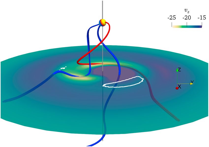
Journal of Geophysical Research: Space Physics 10.1029/2018JA025331

 Figure 2. Run 1: Contours of vz and velocity streamlines in the y = 0 plane (x axis points upward) at t = 8.3trot (left) and
 a quarter of rotation later (right). The orange line represents a distance of 40, from the center of the simulation domain
 to the outer boundary, along the planetary spin axis. The red contours show the location of the reconnection sites
 ( ≥ 15).

 reflections at the x = 0 and y = 0 planes). The pitch of the helical structure of the reconnection sites is roughly
 twice the pitch of the magnetic field lines (≃ 12.5R0 ; see Figure 2). The two structures move downstream at
 the same phase velocity so that at a fixed position downstream of the planet, the temporal periodicity of the
 reconnection sites is twice the temporal periodicity of the magnetic field. At t = 8.3trot (Figure 1, first row) the
 planetary magnetic axis is approximately parallel to the IMF orientation and is therefore favorable for recon-
 nection at the subsolar point (Figure 2, left). During the other phases of the rotation, the reconnection sites
 are localized off axis only. Reconnection sites are places where the IMF and planetary field become connected
 or disconnected. Planetary field lines extending downstream close to the z axis and far from the reconnection
 sites (as for the lines in Figure 1 at t = 8.3trot or t = 8.9trot ) present a neat helical structure with a regular pitch.
 Planetary lines that approach the reconnection sites (particularly visible at t = 8.7trot ) make large excursions
 in the direction perpendicular to z with an essentially vanishing pitch; that is, field components perpendicular
 to z are dominant.
 The z = −15R0 cut of Figure 3 shows that the downstream directed fluid velocity vz (all velocities are normal-
 ized to the sound speed in the solar wind; see section 4) is largest (≃ −25) for these IMF connected field lines.
 Since these field lines are perpendicular to the fluid velocity vector (and the velocity field is incompressible),
 they must travel at the fluid velocity by virtue of the frozen-in theorem. vz = −25 is effectively the asymptotic
 velocity of the whole structure in the downstream region. Figure 3 also shows that planet connected field
 lines of the type shown in Figure 1 at t = 8.7trot (i.e., not connected with the IMF at or upstream of z = −15R0 )
 are embedded in a much slower plasma flowing at vz ≃ −15. These lines thus support an Alfvénic fluctuation
 propagating downstream in the plasma frame at a phase velocity of the order of −10 (−200 km/s in SI units)
 to keep in phase with the global motion of the whole helical structure.
 In general, the helical structure moves downstream faster than the fluid velocity in both the magnetosheath
 and the solar wind. The question is as follows: what determines the overall velocity of the structure (and thus
 the helical pitch)? Some authors suggest that because of the Alfvénic nature of the structure, it should travel
 at the Alfvén speed. In the Tóth et al. (2004) simulations where there is no IMF field and no direct connection
 between the helical structure formed by the planetary field lines and the solar wind, the propagation speed of
 the whole structure (in the plasma frame) should be of the order of the Alfvén speed, especially when the field
 lines are elongated in the z direction as for their much more slowly rotating planet. The discrepancy between
 propagation speed and Alfvén speed in the Tóth et al. (2004) simulations is attributed by the authors to fric-
 tional forces through the magnetopause. In our simulation we do effectively observe that the helical structure
 is formed by propagating Alfvén waves, leaving no doubts about the Alvénic nature of the structure. However,
 we argue that the IMF connected planetary field lines play an essential role in regulating the downstream
 motion of the helical magnetic structure. To verify this intuition, we run our simulations twice, once with the
 IMF, and once with the IMF set to 0 nT. We observe that in the case without IMF, the wavelength of the heli-
 cal structure is constant. However, in the case with IMF, the wavelength of the helical structure has a length

GRITON ET AL. 5399

Journal of Geophysical Research: Space Physics 10.1029/2018JA025331

 Figure 3. Run 1: contours of vz in the z = −15R0 plane (seen from the tail), at t = 8.7trot (top), along with a zoom of the
 black squared area (bottom). The color scheme shows areas flowing tailward slower (blue), faster (yellow to white) than
 the solar wind (traveling at vz = −20). Red and blue stream tracers show a sample of magnetic field lines connected to
 the planet and twisted in a double helix as in Figure 1. These nearly z-aligned field lines are embedded in two distinct
 slowly flowing plasma regions. Each of these two regions is populated with field lines connected to one particular
 magnetic hemisphere of the planet. The white stream tracers show magnetic field lines crossing the rotation axis. They
 are embedded in a fast-flowing plasma and have a small Bz thus separating the slow field regions with different Bz
 polarity. Such lines are either planetary lines connected to the IMF through the magnetopause at the planes location or
 pure planetary lines with each foot connected to a different magnetic hemisphere of the planet. They may also be pure
 IMF lines. In any case these lines do not extend significantly downstream of the plane under consideration. IMF =
 interplanetary magnetic field.

 87% of the length of the corresponding wavelength in the no-IMF simulation, showing that the propagation
 of the helix is slowed down by the IMF.
 The global structure of the magnetic field lines and of the flow pattern is different from usual schemes pro-
 posed for fast rotators in more Earth-like configurations, as Saturn or Jupiter (see chapters 5, 6, and 12 from
 Keiling et al., 2015, and references therein). From our simulation we do extract the following scenario:
 1. IMF field lines that connect to the planetary magnetic field, when upstream or immediately downstream of
 the planet, become retarded by the rotation (such field lines are not visible in Figure 1) with the portion of
 field lines in the magnetosheath in advance with respect to the portion inside the magnetopause.
 2. During the retardation phase, the portion of the field lines inside the magnetopause becomes acceler-
 ated to high tailward velocities by the torque due to the Lorentz force. The lines going through the fast
 flow regions of Figure 3 are representative of such accelerated lines which travel faster than their foot in
 the magnetosheath thus reducing the overall distortion of the retarded field lines. These lines thus slide
 along the surface of the magnetopause at a velocity that is globally larger than the fluid velocity in the

GRITON ET AL. 5400

Journal of Geophysical Research: Space Physics 10.1029/2018JA025331

 Figure 4. Run 2: side view (left column) and associated view from the tail (right column) of a sample of magnetic field
 lines connected to the positive magnetic pole (yellow-to-red lines) and to the negative magnetic pole (cyan-to-blue
 lines). Gray contours delimit volumes where ≥ 20, a proxy for reconnection. The dark line indicates the rotation axis
 (z axis). The x axis points upward in all plots.

 magnetosheath. Eventually, a portion of the field lines encounters a reconnection region (volumes delim-
 ited by gray surfaces in Figure 1) where it disconnects completely from the planet, transforming into a slowly
 moving magnetosheath line.
 3. Other magnetosheath lines, downstream of a reconnection region, may also connect to the planet as the
 reconnection regions move faster than the plasma in the magnetosheath. We argue that as a consequence
 of these exchanges between IMF field and planetary field the helical structure is asymptotically slowed
 down to the magnetosheath plasma velocity (which tends toward the solar wind velocity at large distances
 down the tail). This is based on our comparison between our simulations with and without IMF. However, in
 our simulation with IMF, the downstream extension of the simulation domain is too small to allow for a mea-
 surable deceleration of the helical structure. For example, no significant deceleration of the high-velocity
 spots in Figure 2 could be observed.
 4. In the simulation, the observed tailward velocity of the helical structure is roughly 50% higher than the
 flow velocity in the magnetosheath. We argue that this difference is a function of the time during which a
 planetary magnetic field line stays connected to the IMF. In other words, it depends on the interval of time
 during which the tailward velocity of a portion of the line (transverse to the z axis) is significantly slower

GRITON ET AL. 5401

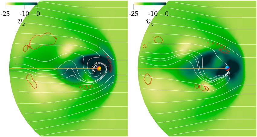
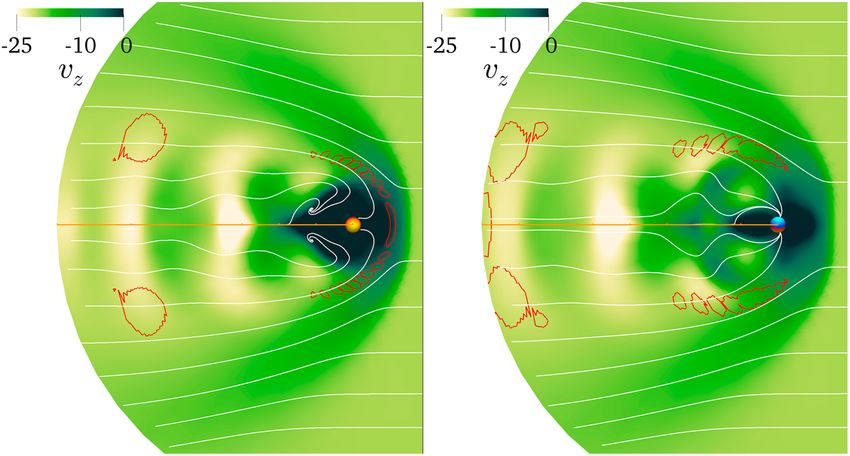
Journal of Geophysical Research: Space Physics 10.1029/2018JA025331

 Figure 5. Run 2: contours of vz and velocity stream lines in the y = 0 plane (x axis points upward) at t = 8.3trot and a
 quarter of rotation later. The orange line represents a distance of 40, from the center of the simulation domain to the
 outer boundary, along the planetary spin axis. The red contours show the location of the reconnection sites ( ≥ 15).

 than its counterpart in the magnetosheath, that is, essentially during the time that the portion of the line
 in the low-velocity region (the dark regions in Figure 2) has a significant transverse component.
 It may be noted that despite the somewhat different spin and magnetic axis orientations, the reconnection
 sites in the simulation are similarly shaped and show a similar temporal variations as in the Masters (2014)
 empirical model (second line in his Figure 5). Here and in Masters’ paper reconnection sites largely cover the
 dayside magnetopause (along a direction parallel to the x axis) at time t = 8.3trot when the IMF and the
 planetary magnetic axis are nearly parallel (case h in Figure 5 of Masters, 2014). No dayside reconnection
 sites are visible half a period later, whereas small, roughly diagonally opposed reconnection spots appear at
 intermediate orientations.
 In Figure 2, the bow shock is visible on the velocity contours, and one may notice that its shape and intensity
 vary over a rotation period (if one compares the figure on the left and the one on the right, a quarter of rota-
 tion later), especially in the dayside. This is a consequence of the change in the reconnection sites location,
 particularly of the subsolar once-per-rotation favorable reconnection site. Figure 2 also illustrates the down-
 stream motion of the reconnection sites (red contours) and the fluid velocity fluctuations in the y = 0 plane.
 In the y = 0 plane, the flow pattern, reconnection sites, and the shape of the bow shock are symmetric by
 construction with respect to the z axis. A symmetry which obviously no longer exists in the 60∘ tilt case will
 be discussed in the next section.

 5.2. The 60∘ Tilt Angle Case
 In Run 2, the helical structure of the connected magnetic field lines is not as clear as in Run 1 (see Figure 4).
 This is a logical consequence of the fact that over a full rotation period one of the planetary poles is always on
 the nightside and the other on the dayside, thus breaking the symmetry between the two poles of Run 1. The
 downstream phase velocity of the structure is the same as in Run 1 (v = −25), so that planetary axis orientation
 does not seem to affect significantly the average pitch of the helical structure once it has been accelerated.
 However, downstream fluid velocities peak at slightly lower levels (as one may notice by comparing Figures 2
 and 5) which is essentially a consequence of the fact that in Run 2 there are no magnetic field lines oriented
 perpendicularly to the z axis in the central region close to the z axis so that fluid and phase velocity do not
 have to be equal.
 Another major difference is the off-z axis displacement of tail structures (evident in all Figures 5–7). As shown
 in Figure 6, the regions with the fastest plasma are now only located off z axis, with no fast streams crossing
 the close to z axis region of slow plasma. The z = −15R0 slice of Figure 7 shows that there are two regions of
 fast plasma regions rotating at different and nonconstant angular velocities so that they sometimes appear to
 merge (e.g., near t = 8.9trot ). The two regions are magnetically connected to each of the two magnetic poles
 of the planet and sometimes to both as at t = 8.5trot . In general, the region connected to the nightside pole
 is spatially well delimited and can be tracked during most of the cycle while the dayside connected region is
 often spread out over a large angular interval.

GRITON ET AL. 5402

Journal of Geophysical Research: Space Physics 10.1029/2018JA025331

 Figure 6. Run 2: slice of the simulation domain at z = −15R0 and t = 8.16trot . The three magnetic field lines are
 connected to the positive planetary magnetic pole (red stream tracer) and to the negative planetary magnetic pole
 (blue stream tracers), respectively. White contours correspond to = 15 and thus delimit reconnection sites. The gray
 vertical line is the rotation axis (z axis). Note that the field lines cross the plane in regions with large and slow fluid
 velocities depending on whether their transverse component is dominant or not.

 At large distances down the tail, beyond the acceleration region, one may use the sign of Bz in order to iden-
 tify the magnetic hemisphere to which the magnetic field lines inside the magnetopause are connected to.
 Figure 8 confirms that at z = −15R0 the magnetic field lines closest to the z axis are all connected to the night-
 side hemisphere of the planet. The dayside connected lines are always located immediately underneath the
 magnetopause so that during some phases of the cycle, as for example at t = 8.5trot , the central region (with
 all lines connected to the nightside planetary hemisphere) is completely surrounded by a region with lines
 having an opposite Bz polarity, some of which (the ones inside the magnetopause) are connected to the day-
 side magnetic hemisphere of the planet. Phases where the innermost region is at least in part surrounded by
 a region of opposite Bz polarity can be observed in Figure 13 of Tóth et al. (2004) even though their Figure 17

 Figure 7. Run 2: slice of the simulation domain at z = −15R0 (seen from the tail with x axis pointing upward), at four
 different times. The magnetic field lines are connected to the positive planetary magnetic pole (red line) or to the
 negative planetary magnetic pole (blue lines) or to both poles (gray lines).

GRITON ET AL. 5403

Journal of Geophysical Research: Space Physics 10.1029/2018JA025331

 Figure 8. Run 2: slice of the simulation domain at z = −15R0 (seen from the tail with x axis pointing upward); yellow-red
 contours indicate areas where Bz < 0, while cyan-blue contours indicate Bz ≥ 0, at four different times. Red and blue
 magnetic field lines are either connected to the positive or the negative planetary magnetic pole. Gray field lines are
 connected to both poles (closed field lines). White contours correspond to = 15 (delimiting reconnection regions). The
 large gray dot shows the rotation axis (z axis).

 does not show a close to z axis region dominated by one single Bz polarity. However, the central part of each
 of the four panels of Figure 8 can be compared with Figures 3a–3c from Schulz and McNab (1996).

 6. Conclusion
 We have presented MHD simulations of the interaction of the solar wind with the magnetosphere of a
 hyperfast-rotating Uranus for solstice orientation of the planetary spin axis, that is, spin axis pointing to the
 Sun. The solar wind is a low-beta, high-Mach number and magnetized plasma with a magnetic field oriented
 perpendicular to the flow velocity. The reason for shortening Uranus rotation period by a factor of 10, thus
 reducing the difference between the rotation period and the Alfvénic crossing time, was double: first, a sub-
 stantial reduction of both computational time and computational domain size with the implied advantage
 of limiting numerical diffusion in time; and second, an enhancement of the effects of the rotation on the
 structure of the magnetospheric tail, as, for example an improved visibility of the reconnection regions due
 to the shortening of the tailward fluctuations of the magnetic field. Obviously, our results cannot be directly
 transposed to the real Uranus as no simple scaling law may exist.
 The first of the two simulations of a hyperfast Uranus is for an unrealistic spin to planetary magnetic axis orien-
 tation of 90∘ . The run has the advantage of presenting a reduced complexity, with the two planetary magnetic
 poles playing a symmetric role. As a consequence of the symmetry of the whole system, the field lines from
 each of the two planetary poles describe two interpenetrating helices stretching downstream of the planet
 (Figure 1). The tailward velocity of the helical structure (≃ 25) is substantially larger than the plasma veloc-
 ity in the solar wind (≃ 20) and in the magnetosheath (≃ 17; Figures 2 and 3). In our simulation the tailward
 velocity of the helical structure is reached within a rather short distance downstream of the planet. That dis-
 tance is of the order of the distance covered by an IMF field line in the magnetosheath during one rotation
 period, which leads us to speculate that the velocity of the helical structure is driven by the IMF field lines
 retarded during the time they are connected to the planet. The fluid velocity in fixed planes transverse to the
 rotation axis is also highly variable in space and time with mostly slow plasma (< 15) near the axis and high
 velocities (> 20) below and at the magnetopause. The helical structure is thus a complex, highly nonlinear,

GRITON ET AL. 5404

Journal of Geophysical Research: Space Physics 10.1029/2018JA025331

 Alfvén wave embedded in a flowing plasma. We speculate that at large downstream distances (beyond
 the boundary of the simulation domain) the velocity of the structure will be asymptotically slowed down
 to the level of the fluid velocity in the magnetosheath. We do not observe such a deceleration in our sim-
 ulation, the downstream region being probably too short, but we argue that the deceleration is inevitable
 because of the field lines in the helical structure connected to the IMF. The most visible illustration of the
 interaction of the helical structure with the IMF are the reconnection regions which in the simulation are
 observed to reach the downstream domain boundary. In the 90∘ run the reconnection regions also show a
 double-helical structure with a pitch 2 times the pitch of the magnetic structure.
 In the second simulation of a hyperfast Uranus we choose spin to planetary magnetic axis of 60∘ , roughly
 the angle of the real planet. Under such circumstances, the two planetary magnetic poles no longer play a
 symmetric role, one pole being always located on the dayside and the other on the nightside of the planet.
 The main consequence is that the nice downstream helical structure of both the magnetic field lines and the
 reconnection region is now broken (Figure 4). In particular, while in the 90∘ case the two reconnection arms
 are always positioned at 180∘ relative to each other in any plane perpendicular to the spin axis, in the 60∘
 case the relative position of the two arms is highly variable. Interestingly, the downstream-directed phase
 speed of the whole structure in the 60∘ simulation is the same as in the 90∘ simulation, probably because the
 magnetic axis orientation is still mainly transverse to both the wind velocity direction and the spin axis. Thus,
 the average helical pitch turns out to be identical in the two simulations. However, in the 60∘ run, the pitch
 tends to be shorter/longer than average depending on the phase (Figures 5–7). As for the symmetric run, no
 significant deceleration of the helical structure could be observed.
 Finally, from the more technical point of view, we have used the background/residual splitting technique of
 the magnetic field for a time-varying background field for the first time in MPI-AMRVAC. We have selected
 the planetary intrinsic magnetic field B0 as the background field which is a time-varying field in the (inertial)
 frame of the simulation. For completeness, the analytic expressions of t B0 for the case of an arbitrary oriented
 multipolar and axisymmetric magnetic field have been extensively presented in section 2.

Acknowledgments References
No new observational data were used
for this work. Simulation results can be Arridge, C. S., Agnor, C. B., André, N., Baines, K. H., Fletcher, L. N., Gautier, D., et al. (2012). Uranus Pathfinder: Exploring the origins and
obtained by contacting the first author. evolution of Ice Giant planets. Experimental Astronomy, 33, 753–791.
The Plas@par project is acknowledged Behannon, K. W., Lepping, R. P., Sittler Jr., E. C., Ness, N. F., Mauk, B. H., Krimigis, S. M., & McNutt, R. L. (1987). The magnetotail of Uranus.
for financial support. The work of Léa Journal of Geophysical Research, 92, 15,354–15,366.
Griton was supported by the CNES Burlaga, L. F., Ness, N. F., Wang, Y.-M., & Sheeley, N. R. (1998). Heliospheric magnetic field strength out to 66 AU: Voyager 1, 1978–1996.
(Centre national d’Etudes spatiales) and Journal of Geophysical Research, 103(A10), 23,727–23,732. https://doi.org/10.1029/98JA01433
the Observatoire de Paris (contract Cao, X., & Paty, C. (2017). Diurnal and seasonal variability of Uranus’s magnetosphere. Journal of Geophysical Research: Space Physics, 122,
reference 5100016058). Some 6318–6331. https://doi.org/10.1002/2017JA024063
computational tests made use of the Chané, E., Saur, J., Keppens, R., & Poedts, S. (2017). How is the Jovian main auroral emission affected by the solar wind?. Journal of
High Performance Computing Geophysical Research: Space Physics, 122, 1960–1978. https://doi.org/10.1002/2016JA023318
OCCIGEN and JADE at CINES within the Connerney, J. E. P., Acuña, M. H., & Ness, N. F. (1987). The magnetic field of Uranus. Journal of Geophysical Research, 92(A13), 15,329–15,336.
DARI project c2015046842. The authors https://doi.org/10.1029/JA092iA13p15329
thank Michel Moncuquet for his helpful Gombosi, T. I., Tóth, G., Zeeuw, D. L. D., Hansen, K. C., Kabin, K., & Powell, K. G. (2002). Semirelativistic magnetohy-
comments. drodynamics and physics-based convergence acceleration. Journal of Computational Physics, 177(1), 176–205.
 http://www.sciencedirect.com/science/article/pii/S0021999102970099
 Jia, X., Hansen, K. C., Gombosi, T. I., Kivelson, M. G., Tóth, G., DeZeeuw, D. L., & Ridley, A. J. (2012). Magnetospheric configuration
 and dynamics of Saturn’s magnetosphere: A global MHD simulation. Journal of Geophysical Research, 117, A05225.
 https://doi.org/10.1029/2012JA017575
 Keiling, A., Jackman, C. M., & Delamere, P. A. (Eds.) (2015). Magnetotails in the solar system, Geophysical Monograph Series (Vol. 207).
 Washington, DC: American Geophysical Union.
 Keppens, R., Meliani, Z., van Marle, A. J., Delmont, P., Vlasis, A., & van der Holst, B. (2012). Parallel, grid-adaptive
 approaches for relativistic hydro and magnetohydrodynamics. Journal of Computational Physics, 231(3), 718–744.
 http://www.sciencedirect.com/science/article/pii/S0021999111000386, Special Issue: Computational Plasma Physics.
 Masters, A. (2014). Magnetic reconnection at Uranus’ magnetopause. Journal of Geophysical Research: Space Physics, 119, 5520–5538.
 https://doi.org/10.1002/2014JA020077
 Podolak, M., & Reynolds, R. T. (1987). The rotation rate of Uranus, its internal structure, and the process of planetary accretion. Icarus, 70,
 31–36.
 Richardson, J. D., & Smith, C. W. (2003). The radial temperature profile of the solar wind. Geophysical Research Letters, 30, 1206.
 https://doi.org/10.1029/2002GL016551
 Schulz, M., & McNab, M. C. (1996). Source-surface modeling of planetary magnetospheres. Journal of Geophysical Research, 101, 5095–5118.
 Tanaka, T. (1994). Finite volume TVD scheme on an unstructured grid system for three-dimensional MHD simulation of inhomogeneous
 systems including strong background potential fields. Journal of Computational Physics, 111(2), 381–389.
 http://www.sciencedirect.com/science/article/pii/S0021999184710710
 Tóth, G., Kovács, D., Hansen, K. C., & Gombosi, T. I. (2004). Three-dimensional MHD simulations of the magnetosphere of Uranus. Journal of
 Geophysical Research, 109, A11210. https://doi.org/10.1029/2004JA010406

GRITON ET AL. 5405

Journal of Geophysical Research: Space Physics 10.1029/2018JA025331

 Voight, G.-H., Behannon, K. W., & Ness, N. F. (1987). Magnetic field and current structures in the magnetosphere of Uranus. Journal of
 Geophysical Research, 92, 15,337–15,346.
 Voight, G.-H., Hill, T. W., & Dessler, A. J. (1983). The magnetosphere of Uranus—Plasma sources, convection, and field configuration.
 The Astrophysical Journal (ApJ), 266, 390–401.

GRITON ET AL. 5406