Movement Pruning: Adaptive Sparsity by Fine-Tuning - NIPS Proceedings
←
→
Page content transcription
If your browser does not render page correctly, please read the page content below
Movement Pruning:
                   Adaptive Sparsity by Fine-Tuning

                      Victor Sanh1 , Thomas Wolf1 , Alexander M. Rush1,2
                              1
                                Hugging Face, 2 Cornell University
                  {victor,thomas}@huggingface.co ; arush@cornell.edu

                                              Abstract
         Magnitude pruning is a widely used strategy for reducing model size in pure
         supervised learning; however, it is less effective in the transfer learning regime that
         has become standard for state-of-the-art natural language processing applications.
         We propose the use of movement pruning, a simple, deterministic first-order weight
         pruning method that is more adaptive to pretrained model fine-tuning. We give
         mathematical foundations to the method and compare it to existing zeroth- and
         first-order pruning methods. Experiments show that when pruning large pretrained
         language models, movement pruning shows significant improvements in high-
         sparsity regimes. When combined with distillation, the approach achieves minimal
         accuracy loss with down to only 3% of the model parameters.

1   Introduction
Large-scale transfer learning has become ubiquitous in deep learning and achieves state-of-the-art
performance in applications in natural language processing and related fields. In this setup, a large
model pretrained on a massive generic dataset is then fine-tuned on a smaller annotated dataset to
perform a specific end-task. Model accuracy has been shown to scale with the pretrained model and
dataset size [Raffel et al., 2019]. However, significant resources are required to ship and deploy these
large models, and training the models have high environmental costs [Strubell et al., 2019].
Sparsity induction is a widely used approach to reduce the memory footprint of neural networks at
only a small cost of accuracy. Pruning methods, which remove weights based on their importance,
are a particularly simple and effective method for compressing models. Smaller models are easier to
sent on edge devices such as mobile phones but are also significantly less energy greedy: the majority
of the energy consumption comes from fetching the model parameters from the long term storage of
the mobile device to its volatile memory [Han et al., 2016a, Horowitz, 2014].
Magnitude pruning [Han et al., 2015, 2016b], which preserves weights with high absolute values, is
the most widely used method for weight pruning. It has been applied to a large variety of architectures
in computer vision [Guo et al., 2016], in language processing [Gale et al., 2019], and more recently
has been leveraged as a core component in the lottery ticket hypothesis [Frankle et al., 2020].
While magnitude pruning is highly effective for standard supervised learning, it is inherently less
useful in the transfer learning regime. In supervised learning, weight values are primarily determined
by the end-task training data. In transfer learning, weight values are mostly predetermined by the
original model and are only fine-tuned on the end task. This prevents these methods from learning to
prune based on the fine-tuning step, or “fine-pruning.”
In this work, we argue that to effectively reduce the size of models for transfer learning, one should
instead use movement pruning, i.e., pruning approaches that consider the changes in weights during
fine-tuning. Movement pruning differs from magnitude pruning in that both weights with low and
high values can be pruned if they shrink during training. This strategy moves the selection criteria

34th Conference on Neural Information Processing Systems (NeurIPS 2020), Vancouver, Canada.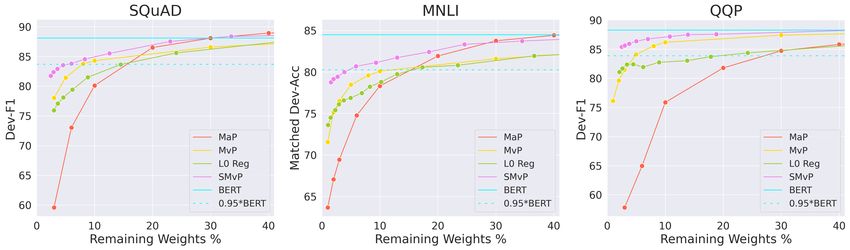
from the 0th to the 1st-order and facilitates greater pruning based on the fine-tuning objective. To
test this approach, we introduce a particularly simple, deterministic version of movement pruning
utilizing the straight-through estimator [Bengio et al., 2013].
We apply movement pruning to pretrained language representations (BERT) [Devlin et al., 2019,
Vaswani et al., 2017] on a diverse set of fine-tuning tasks. In highly sparse regimes (less than 15% of
remaining weights), we observe significant improvements over magnitude pruning and other 1st-order
methods such as L0 regularization [Louizos et al., 2017]. Our models reach 95% of the original
BERT performance with only 5% of the encoder’s weight on natural language inference (MNLI)
[Williams et al., 2018] and question answering (SQuAD v1.1) [Rajpurkar et al., 2016]. Analysis of
the differences between magnitude pruning and movement pruning shows that the two methods lead
to radically different pruned models with movement pruning showing greater ability to adapt to the
end-task.

2   Related Work
In addition to magnitude pruning, there are many other approaches for generic model weight pruning.
Most similar to our approach are methods for using parallel score matrices to augment the weight
matrices [Mallya and Lazebnik, 2018, Ramanujan et al., 2020], which have been applied for convo-
lutional networks. Differing from our methods, these methods keep the weights of the model fixed
(either from a randomly initialized network or a pre-trained network) and the scores are updated to
find a good sparse subnetwork.
Many previous works have also explored using higher-order information to select prunable weights.
LeCun et al. [1989] and Hassibi et al. [1993] leverage the Hessian of the loss to select weights for
deletion. Our method does not require the (possibly costly) computation of second-order derivatives
since the importance scores are obtained simply as the by-product of the standard fine-tuning. [Theis
et al., 2018, Ding et al., 2019, Lee et al., 2019] use the absolute value or the square value of the
gradient. In contrast, we found it useful to preserve the direction of movement in our algorithm.
Compressing pretrained language models for transfer learning is also a popular area of study. Other
approaches include knowledge distillation [Sanh et al., 2019, Tang et al., 2019] and structured pruning
[Fan et al., 2020a, Sajjad et al., 2020, Michel et al., 2019, Wang et al., 2019]. Our core method does
not require an external teacher model and targets individual weight. We also show that having a
teacher can further improve our approach. Recent work also builds upon iterative magnitude pruning
with rewinding [Yu et al., 2020], weight redistribution [Dettmers and Zettlemoyer, 2019] models
from scratch. This differs from our approach which we frame in the context of transfer learning
(focusing on the fine-tuning stage). Finally, another popular compression approach is quantization.
Quantization has been applied to a variety of modern large architectures [Fan et al., 2020b, Zafrir
et al., 2019, Gong et al., 2014] providing high memory compression rates at the cost of no or little
performance. As shown in previous works [Li et al., 2020, Han et al., 2016b] quantization and
pruning are complimentary and can be combined to further improve the performance/size ratio.

3   Background: Score-Based Pruning
We first establish shared notation for discussing different neural network pruning strategies. Let
W ∈ Rn×n refer to a generic weight matrix in the model (we consider square matrices, but they
could be of any shape). To determine which weights are pruned, we introduce a parallel matrix of
associated importance scores S ∈ Rn×n . Given importance scores, each pruning strategy computes a
mask M ∈ {0, 1}n×n . Inference for an input x becomes a = (W M)x, where is the Hadamard
product. A common strategy is to keep the top-v percent of weights by importance. We define Topv
as a function which selects the v% highest values in S:

                                                 1, Si,j in top v%
                                 Topv (S)i,j =                                                 (1)
                                                 0, o.w.

Magnitude-based weight pruning determines the mask based on the absolute value
                                                                                of each weight
as a measure of importance. Formally, we have importance scores S = |Wi,j | 1≤i,j≤n , and masks
M = Topv (S) (Eq (1)). There are several extensions to this base setup. Han et al. [2015] use

                                                  2
Magnitude pruning                  L0 regularization           Movement pruning      Soft movement pruning
 Pruning Decision            0th order                      1st order                     1st order              1st order
 Masking Function              Topv                 Continuous Hard-Concrete                Topv               Thresholding
 Pruning Structure        Local or Global                     Global                   Local or Global            Global
 Learning Objective              L                        L + λl0 E(L0 )                      L               L + λmvp R(S)
 Gradient Form                                          Gumbel-Softmax                Straight-Through       Straight-Through
                                                     P ∂L (t) (t)            (t)      P ∂L (t) (t)           P ∂L (t) (t)
 Scores S                     |Wi,j |               − t ( ∂W i,j
                                                                 ) Wi,j f (S i,j )   − t ( ∂W i,j
                                                                                                  ) Wi,j    − t ( ∂W i,j
                                                                                                                         ) Wi,j

Table 1: Summary of the pruning methods considered in this work and their specificities. The
expression of f of L0 regularization is detailed in Eq (4).

iterative magnitude pruning: the model is first trained until convergence and weights with the lowest
magnitudes are removed afterward. The sparsified model is then re-trained with the removed weights
fixed to 0. This loop is repeated until the desired sparsity level is reached.
In this study, we focus on automated gradual pruning [Zhu and Gupta, 2018]. It supplements
magnitude pruning by allowing masked weights to be updated such that they are not fixed for the
entire duration of the training. Automated gradual pruning enables the model to recover from previous
masking choices [Guo et al., 2016]. In addition, one can gradually increases the sparsity level v
                                                                                         t−ti 3

during training using a cubic sparsity scheduler: v (t) = vf + (vi − vf ) 1 − N            ∆t . The sparsity
level at time step t, v (t) is increased from an initial value vi (usually 0) to a final value vf in n pruning
steps after ti steps of warm-up. The model is thus pruned and trained jointly.

4       Movement Pruning
Magnitude pruning can be seen as utilizing zeroth-order information (absolute value) of the running
model. In this work, we focus on movement pruning methods where importance is derived from
first-order information. Intuitively, instead of selecting weights that are far from zero, we retain
connections that are moving away from zero during the training process. We consider two versions of
movement pruning: hard and soft.
For (hard) movement pruning, masks are computed using the Topv function: M = Topv (S). Unlike
                                                   Pnweights W and their importance scores S.
magnitude pruning, during training, we learn both the
During the forward pass, we compute for all i, ai = k=1 Wi,k Mi,k xk .
Since the gradient of Topv is 0 everywhere it is defined, we follow Ramanujan et al. [2020], Mallya
and Lazebnik [2018] and approximate its value with the straight-through estimator [Bengio et al.,
2013]. In the backward pass, Topv is ignored and the gradient goes "straight-through" to S. The
approximation of gradient of the loss L with respect to Si,j is given by
                                               ∂L     ∂L ∂ai      ∂L
                                                    =           =     Wi,j xj                                                 (2)
                                              ∂Si,j   ∂ai ∂Si,j   ∂ai
This implies that the scores of weights are updated, even if these weights are masked in the forward
pass. We prove in Appendix A.1 that movement pruning as an optimization problem will converge.
We also consider a relaxed (soft) version of movement pruning based on the binary mask function
described by Mallya and Lazebnik [2018]. Here we replace hyperparameter v with a fixed global
threshold value τ that controls the binary mask. The mask is calculated
                                                                      Pas M = (S > τ ). In order to
control the sparsity level, we add a regularization term R(S) = λmvp i,j σ(Si,j ) which encourages
the importance scores to decrease over time1 . The coefficient λmvp controls the penalty intensity and
thus the sparsity level.

Method Interpretation In movement pruning, the gradient of L with respect to Wi,j is given
                                      ∂L      ∂L
by the standard gradient derivation: ∂W i,j
                                            = ∂ai
                                                  Mi,j xj . By combining it to Eq (2), we have
 ∂L           ∂L
∂Si,j    =   ∂Wi,j Wi,j   (we omit the binary mask term Mi,j for simplicity). From the gradient update in
                                             ∂L
Eq (2), Si,j is increasing when             ∂Si,j    < 0, which happens in two cases:
    1                                   P
        We also experimented with           i,j   |Si,j | but it turned out to be harder to tune while giving similar results.

                                                                     3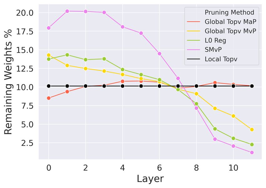
(a) Magnitude pruning                   (b) Movement pruning
Figure 1: During fine-tuning (on MNLI), the weights stay close to their pre-trained values which
limits the adaptivity of magnitude pruning. We plot the identity line in black. Pruned weights are
plotted in grey. Magnitude pruning selects weights that are far from 0 while movement pruning
selects weights that are moving away from 0.

               ∂L
      • (a)   ∂Wi,j   < 0 and Wi,j > 0
               ∂L
      • (b)   ∂Wi,j   > 0 and Wi,j < 0

It means that during training Wi,j is increasing while being positive or is decreasing while being
negative. It is equivalent to saying that Si,j is increasing when Wi,j is moving away from 0. Inversely,
                            ∂L
Si,j is decreasing when ∂S    i,j
                                  > 0 which means that Wi,j is shrinking towards 0.
While magnitude pruning selects the most important weights as the ones which maximize their
distance to 0 (|Wi,j |), movement pruning selects the weights which are moving the most away from
0 (Si,j ). For this reason, magnitude pruning can be seen as a 0th order method, whereas movement
pruning is based on a 1st order signal. In fact, S can be seen as an accumulator of movement: from
equation (2), after T gradient updates, we have
                                    (T )
                                                 X ∂L             (t)
                                   Si,j = −αS       (       )(t) Wi,j                           (3)
                                                      ∂Wi,j
                                                t 0, l < 0, and r > 1:

              u ∼ U(0, 1)                     S i,j = σ (log(u) − log(1 − u) + Si,j )/b
           Zi,j = (r − l)S i,j + l            Mi,j = min(1, ReLU(Zi,j ))

P expected L0 norm has a closed
The                               form involving the parameters of the hard-concrete: E(L0 ) =
  i,j σ log Si,j − b log(−l/r) . Thus, the weights and scores of the model can be optimized in

                                                   4
an end-to-end fashion to minimize the sum of the training loss L and the expected L0 penalty. A
coefficient λl0 controls the L0 penalty and indirectly the sparsity level. Gradients take a similar form:
∂L ∂L r−l
= Wi,j xj f (S i,j ) where f (S i,j ) = S̄i,j (1 − S̄i,j )1{0≤Zi,j ≤1} (4)
∂Si,j ∂ai b
At test time, a non-stochastic estimation of the mask is used: M̂ = min 1, ReLU (r − l)σ(S) + l
and weights multiplied by 0 can simply be discarded.
Table 1 highlights the characteristics of each pruning method. The main differences are in the masking
functions, pruning structure, and the final gradient form.
5 Experimental Setup
Transfer learning for NLP uses large pre-trained language models that are fine-tuned on target tasks
[Ruder et al., 2019, Devlin et al., 2019, Radford et al., 2019, Liu et al., 2019]. We experiment
with task-specific pruning of BERT-base-uncased, a pre-trained model that contains roughly 84M
parameters. We freeze the embedding modules and fine-tune the transformer layers and the task-
specific head. All reported sparsity percentages are relative to BERT-base and correspond exactly to
model size even comparing to baselines.
We perform experiments on three monolingual (English) tasks, which are common benchmarks for
the recent progress in transfer learning for NLP: question answering (SQuAD v1.1) [Rajpurkar et al.,
2016], natural language inference (MNLI) [Williams et al., 2018], and sentence similarity (QQP)
[Iyer et al., 2017]. The datasets respectively contain 8K, 393K, and 364K training examples. SQuAD
is formulated as a span extraction task, MNLI and QQP are paired sentence classification tasks.
For a given task, we fine-tune the pre-trained model for the same number of updates (between 6
and 10 epochs) across pruning methods2 . We follow Zhu and Gupta [2018] and use a cubic sparsity
scheduling for Magnitude Pruning (MaP), Movement Pruning (MvP), and Soft Movement Pruning
(SMvP). Adding a few steps of cool-down at the end of pruning empirically improves the performance
especially in high sparsity regimes. The schedule for v is:
vi 0 ≤ t < ti
t−ti −tf 3
v + (vi − vf )(1 − N ∆t ) ti ≤ t < T − tf (5)
f
vf o.w.
where tf is the number of cool-down steps.
We compare our results against several state-of-the-art pruning baselines: Reweighted Proximal
Pruning (RPP) [Guo et al., 2019] combines re-weighted L1 minimization and Proximal Projection
[Parikh and Boyd, 2014] to perform unstructured pruning. LayerDrop [Fan et al., 2020a] leverages
structured dropout to prune models at test time. For RPP and LayerDrop, we report results from
authors. We also compare our method against the mini-BERT models, a collection of smaller BERT
models with varying hyper-parameters [Turc et al., 2019].
Finally, Gordon et al. [2020], Li et al. [2020] apply unstructured magnitude pruning as a post-hoc
operation whereas we use automated gradual pruning [Zhu and Gupta, 2018] which improves on
these methods by enabling masked weights to be updated. Moreover, McCarley [2019] compares
multiple methods to compute structured masking (L0 regularization and head importance as described
in [Michel et al., 2019]) and found that structured L0 regularization performs best. We did not find
any implementation for this work, so for fair comparison, we presented a strong unstructured L0
regularization baseline.
6 Results
Figure 2 displays the results for the main pruning methods at different levels of pruning on each
dataset. First, we observe the consistency of the comparison between magnitude and movement
2
Preliminary experiments showed that increasing the number of pruning steps tended to improve the end
performance
5Figure 2: Comparisons between different pruning methods in high sparsity regimes. Soft movement
pruning consistently outperforms other methods in high sparsity regimes. We plot the perfor-
mance of the standard fine-tuned BERT along with 95% of its performance. Sparsity percentages are
relative to BERT-base and correspond exactly to model size.
Table 2: Performance at high sparsity levels. (Soft) movement pruning outperforms current state-
of-the art pruning methods at different high sparsity levels. 3% corresponds to 2.6 millions (M)
non-zero parameters in the encoder and 10% to 8.5M.
BERT base Remaining
fine-tuned Weights (%) MaP L0 Regu MvP soft MvP
SQuAD - Dev 10% 67.7/78.5 69.9/80.0 71.9/81.7 71.3/81.5
80.4/88.1
EM/F1 3% 40.1/54.5 61.2/73.3 65.2/76.3 69.5/79.9
MNLI - Dev 10% 77.8/79.0 77.9/78.5 79.3/79.5 80.7/81.1
acc/MM acc 84.5/84.9
3% 68.9/69.8 75.1/75.4 76.1/76.7 79.0/79.6
QQP - Dev 10% 78.8/75.1 87.5/81.9 89.1/85.5 90.5/87.1
91.4/88.4
acc/F1 3% 72.1/58.4 86.5/81.0 85.6/81.0 89.3/85.6
pruning: at low sparsity (more than 70% of remaining weights), magnitude pruning outperforms
all methods with little or no loss with respect to the dense model whereas the performance of
movement pruning methods quickly decreases even for low sparsity levels. However, magnitude
pruning performs poorly with high sparsity, and the performance drops extremely quickly. In contrast,
first-order methods show strong performances with less than 15% of remaining weights.
Table 2 shows the specific model scores for different methods at high sparsity levels. Magnitude
pruning on SQuAD achieves 54.5 F1 with 3% of the weights compared to 73.3 F1 with L0 regular-
ization, 76.3 F1 for movement pruning, and 79.9 F1 with soft movement pruning. These experiments
indicate that in high sparsity regimes, importance scores derived from the movement accumulated
during fine-tuning induce significantly better pruned models compared to absolute values.
Next, we compare the difference in performance between first-order methods. We see that straight-
through based hard movement pruning (MvP) is comparable with L0 regularization (with a significant
gap in favor of movement pruning on QQP). Soft movement pruning (SMvP) consistently outperforms
hard movement pruning and L0 regularization by a strong margin and yields the strongest performance
among all pruning methods in high sparsity regimes. These comparisons support the fact that even if
movement pruning (and its relaxed version soft movement pruning) is simpler than L0 regularization,
it yet yields stronger performances for the same compute budget.
Finally, movement pruning and soft movement pruning compare favorably to the other baselines, ex-
cept for QQP where RPP is on par with soft movement pruning. Movement pruning also outperforms
the fine-tuned mini-BERT models. This is coherent with [Li et al., 2020]: it is both more efficient and
more effective to train a large model and compress it afterward than training a smaller model from
scratch. We do note though that current hardware does not support optimized inference for sparse
models: from an inference speed perspective, it might often desirable to use a small dense model
such as mini-BERT over a sparse alternative of the same size.
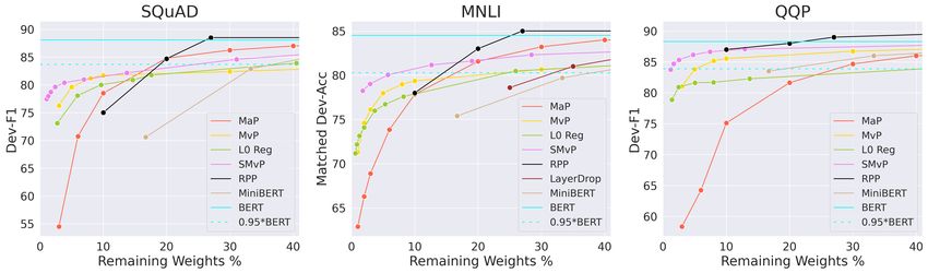
Distillation further boosts performance Following previous work, we can further leverage knowl-
edge distillation [Bucila et al., 2006, Hinton et al., 2014] to boost performance for free in the pruned
domain [Jiao et al., 2019, Sanh et al., 2019] using our baseline fine-tuned BERT-base model as
6Figure 3: Comparisons between different pruning methods augmented with distillation. Distillation
improves the performance across all pruning methods and sparsity levels.
Table 3: Distillation-augmented performances for selected high sparsity levels. All pruning methods
benefit from distillation signal further enhancing the ratio Performance VS Model Size.
BERT base Remaining
fine-tuned Weights (%) MaP L0 Regu MvP soft MvP
SQuAD - Dev 10% 70.2/80.1 72.4/81.9 75.6/84.3 76.6/84.9
80.4/88.1
EM/F1 3% 45.5/59.6 64.3/75.8 67.5/78.0 72.7/82.3
MNLI - Dev 10% 78.3/79.3 78.7/79.7 80.1/80.4 81.2/81.8
acc/MM acc 84.5/84.9
3% 69.4/70.6 76.0/76.2 76.5/77.4 79.5/80.1
QQP - Dev 10% 79.8/65.0 88.1/82.8 89.7/86.2 90.2/86.8
91.4/88.4
acc/F1 3% 72.4/57.8 87.0/81.9 86.1/81.5 89.1/85.5
teacher. The training objective is a convex combination of the training loss and a knowledge distilla-
tion loss on the output distributions. Figure 3 shows the results on SQuAD, MNLI, and QQP for the
three pruning methods boosted with distillation. Overall, we observe that the relative comparisons
of the pruning methods remain unchanged while the performances are strictly increased. Table 3
shows for instance that on SQuAD, movement pruning at 10% goes from 81.7 F1 to 84.3 F1. When
combined with distillation, soft movement pruning yields the strongest performances across all
pruning methods and studied datasets: it reaches 95% of BERT-base with only a fraction of the
weights in the encoder (∼5% on SQuAD and MNLI).
7 Analysis
(a) Distribution of remaining weights (b) Scores and weights learned by
movement pruning
Figure 4: Magnitude pruning and movement pruning leads to pruned models with radically different
weight distribution.
7Figure 5: Comparison of local and global selec- Figure 6: Remaining weights per layer in the
tions of weights on SQuAD at different sparsity Transformer. Global magnitude pruning tends to
levels. For magnitude and movement pruning, prune uniformly layers. Global 1st order meth-
local and global Topv performs similarly at all ods allocate the weight to the lower layers while
levels of sparsity. heavily pruning the highest layers.
Movement pruning is adaptive Figure 4a compares the distribution of the remaining weights for
the same matrix of a model pruned at the same sparsity using magnitude and movement pruning. We
observe that by definition, magnitude pruning removes all the weights that are close to zero, ending
up with two clusters. In contrast, movement pruning leads to a smoother distribution, which covers
the whole interval except for values close to 0.
Figure 4b displays each individual weight against its associated importance score in movement
pruning. We plot pruned weights in grey. We observe that movement pruning induces no simple
relationship between the scores and the weights. Both weights with high absolute value or low
absolute value can be considered important. However, high scores are systematically associated with
non-zero weights (and thus the “v-shape”). This is coherent with the interpretation we gave to the
scores (section 4): a high score S indicates that during fine-tuning, the associated weight moved away
from 0 and is thus non-null.
Local and global masks perform similarly We study the influence of the locality of the pruning
decision. While local Topv selects the v% most important weights matrix by matrix, global Topv
uncovers non-uniform sparsity patterns in the network by selecting the v% most important weights in
the whole network. Previous work has shown that a non-uniform sparsity across layers is crucial to
the performance in high sparsity regimes [He et al., 2018]. In particular, Mallya and Lazebnik [2018]
found that the sparsity tends to increase with the depth of the network layer.
Figure 5 compares the performance of local selection (matrix by matrix) against global selection
(all the matrices) for magnitude pruning and movement pruning. Despite being able to find a
global sparsity structure, we found that global did not significantly outperform local, except in high
sparsity regimes (2.3 F1 points of difference with 3% of remaining weights for movement pruning).
Even though the distillation signal boosts the performance of pruned models, the end performance
difference between local and global selections remains marginal.
Figure 6 shows the remaining weights percentage obtained per layer when the model is pruned until
10% with global pruning methods. Global weight pruning is able to allocate sparsity non-uniformly
through the network, and it has been shown to be crucial for the performance in high sparsity regimes
[He et al., 2018]. We notice that except for global magnitude pruning, all the global pruning methods
tend to allocate a significant part of the weights to the lowest layers while heavily pruning in the
highest layers. Global magnitude pruning tends to prune similarly to local magnitude pruning, i.e.,
uniformly across layers.
88 Conclusion
We consider the case of pruning of pretrained models for task-specific fine-tuning and compare
zeroth- and first-order pruning methods. We show that a simple method for weight pruning based on
straight-through gradients is effective for this task and that it adapts using a first-order importance
score. We apply this movement pruning to a transformer-based architecture and empirically show that
our method consistently yields strong improvements over existing methods in high-sparsity regimes.
The analysis demonstrates how this approach adapts to the fine-tuning regime in a way that magnitude
pruning cannot. In future work, it would also be interesting to leverage group-sparsity inducing
penalties [Bach et al., 2011] to remove entire columns or filters. In this setup, we would associate a
score to a group of weights (a column or a row for instance). In the transformer architecture, it would
give a systematic way to perform feature selection and remove entire columns of the embedding
matrix.
9 Broader Impact
This work is part of a broader line of research on reducing the memory size of state-of-the-art models
in Natural Language Processing (and more generally in Artificial Intelligence). This line of research
has potential positive impact in society from a privacy and security perspective: being able to store
and run state-of-the-art NLP capabilities on devices (such as smartphones) would erase the need to
send API calls (with potentially private data) to a remote server. It is particularly important since
there is a rising concern about the potential negative uses of centralized personal data. Moreover, this
is complementary to hardware manufacturers’ efforts to build chips that will considerably speedup
inference for sparse networks while reducing the energy consumption of such networks.
From an accessibility standpoint, this line of research has the potential to give access to extremely
large models [Raffel et al., 2019, Brown et al., 2020] to the broader community, and not only big
labs with large clusters. Extremely compressed models with comparable performance enable smaller
teams or individual researchers to experiment with large models on a single GPU. For instance, it
would enable the broader community to engage in analyzing a model’s biases such as gender bias [Lu
et al., 2018, Vig et al., 2020], or a model’s lack of robustness to adversarial attacks [Wallace et al.,
2019]. More in-depth studies are necessary in these areas to fully understand the risks associated to a
model and create robust ways to mitigate them before massively deploying these capabilities.
Acknowledgments and Disclosure of Funding
This work is conducted as part the authors’ employment at Hugging Face.
References
Colin Raffel, Noam Shazeer, Adam Roberts, Katherine Lee, Sharan Narang, Michael Matena, Yanqi
Zhou, Wei Li, and Peter J. Liu. Exploring the limits of transfer learning with a unified text-to-text
transformer. ArXiv, abs/1910.10683, 2019.
Emma Strubell, Ananya Ganesh, and Andrew McCallum. Energy and policy considerations for deep
learning in nlp. In ACL, 2019.
Song Han, Xingyu Liu, Huizi Mao, Jing Pu, Ardavan Pedram, Mark Horowitz, and William J. Dally.
Eie: Efficient inference engine on compressed deep neural network. In ISCA, 2016a.
M. Horowitz. 1.1 computing’s energy problem (and what we can do about it). In ISSCC, 2014.
Song Han, Jeff Pool, John Tran, and William J. Dally. Learning both weights and connections for
efficient neural network. In NIPS, 2015.
Song Han, Huizi Mao, and William J. Dally. Deep compression: Compressing deep neural network
with pruning, trained quantization and huffman coding. In ICLR, 2016b.
Yiwen Guo, Anbang Yao, and Yurong Chen. Dynamic network surgery for efficient dnns. In NIPS,
2016.
9Trevor Gale, Erich Elsen, and Sara Hooker. The state of sparsity in deep neural networks. ArXiv,
abs/1902.09574, 2019.
Jonathan Frankle, G. Dziugaite, D. M. Roy, and Michael Carbin. Linear mode connectivity and the
lottery ticket hypothesis. In ICML, 2020.
Yoshua Bengio, Nicholas Léonard, and Aaron C. Courville. Estimating or propagating gradients
through stochastic neurons for conditional computation. ArXiv, abs/1308.3432, 2013.
Jacob Devlin, Ming-Wei Chang, Kenton Lee, and Kristina Toutanova. Bert: Pre-training of deep
bidirectional transformers for language understanding. In NAACL, 2019.
Ashish Vaswani, Noam Shazeer, Niki Parmar, Jakob Uszkoreit, Llion Jones, Aidan N. Gomez, Lukasz
Kaiser, and Illia Polosukhin. Attention is all you need. In NIPS, 2017.
Christos Louizos, Max Welling, and Diederik P. Kingma. Learning sparse neural networks through
l0 regularization. In ICLR, 2017.
Adina Williams, Nikita Nangia, and Samuel Bowman. A broad-coverage challenge corpus for
sentence understanding through inference. In NAACL, 2018.
Pranav Rajpurkar, Jian Zhang, Konstantin Lopyrev, and Percy Liang. Squad: 100, 000+ questions for
machine comprehension of text. In EMNLP, 2016.
Arun Mallya and Svetlana Lazebnik. Piggyback: Adding multiple tasks to a single, fixed network by
learning to mask. ArXiv, abs/1801.06519, 2018.
Vivek Ramanujan, Mitchell Wortsman, Aniruddha Kembhavi, Ali Farhadi, and Mohammad Rastegari.
What’s hidden in a randomly weighted neural network? In CVPR, 2020.
Yann LeCun, John S. Denker, and Sara A. Solla. Optimal brain damage. In NIPS, 1989.
Babak Hassibi, David G. Stork, and Gregory J. Wolff. Optimal brain surgeon: Extensions and
performance comparisons. In NIPS, 1993.
Lucas Theis, Iryna Korshunova, Alykhan Tejani, and Ferenc Huszár. Faster gaze prediction with
dense networks and fisher pruning. ArXiv, abs/1801.05787, 2018.
Xiaohan Ding, Guiguang Ding, Xiangxin Zhou, Yuchen Guo, Ji Liu, and Jungong Han. Global sparse
momentum sgd for pruning very deep neural networks. In NeurIPS, 2019.
Namhoon Lee, Thalaiyasingam Ajanthan, and Philip H. S. Torr. Snip: Single-shot network pruning
based on connection sensitivity. In ICLR, 2019.
Victor Sanh, Lysandre Debut, Julien Chaumond, and Thomas Wolf. Distilbert, a distilled version of
bert: smaller, faster, cheaper and lighter. In NeurIPS EMC2 Workshop, 2019.
Raphael Tang, Yao Lu, Linqing Liu, Lili Mou, Olga Vechtomova, and Jimmy Lin. Distilling
task-specific knowledge from bert into simple neural networks. ArXiv, abs/1903.12136, 2019.
Angela Fan, Edouard Grave, and Armand Joulin. Reducing transformer depth on demand with
structured dropout. In ICLR, 2020a.
Hassan Sajjad, Fahim Dalvi, Nadir Durrani, and Preslav Nakov. Poor man’s bert: Smaller and faster
transformer models. ArXiv, abs/2004.03844, 2020.
Paul Michel, Omer Levy, and Graham Neubig. Are sixteen heads really better than one? In NeurIPS,
2019.
Ziheng Wang, Jeremy Wohlwend, and Tao Lei. Structured pruning of large language models. ArXiv,
abs/1910.04732, 2019.
Haonan Yu, Sergey Edunov, Yuandong Tian, and Ari S. Morcos. Playing the lottery with rewards and
multiple languages: lottery tickets in rl and nlp. In ICLR, 2020.
10Tim Dettmers and L. Zettlemoyer. Sparse networks from scratch: Faster training without losing
performance. ArXiv, abs/1907.04840, 2019.
Angela Fan, Pierre Stock, Benjamin Graham, Edouard Grave, Rémi Gribonval, Hervé Jégou,
and Armand Joulin. Training with quantization noise for extreme model compression. ArXiv,
abs/2004.07320, 2020b.
Ofir Zafrir, Guy Boudoukh, Peter Izsak, and Moshe Wasserblat. Q8bert: Quantized 8bit bert. In
NeurIPS EMC2 Workshop, 2019.
Yunchao Gong, Liu Liu, Ming Yang, and Lubomir D. Bourdev. Compressing deep convolutional
networks using vector quantization. ArXiv, abs/1412.6115, 2014.
Zhuohan Li, Eric Wallace, Sheng Shen, Kevin Lin, Kurt Keutzer, Dan Klein, and Joseph E. Gon-
zalez. Train large, then compress: Rethinking model size for efficient training and inference of
transformers. In ICML, 2020.
Michael Zhu and Suyog Gupta. To prune, or not to prune: exploring the efficacy of pruning for model
compression. In ICLR, 2018.
Mitchell A. Gordon, Kevin Duh, and Nicholas Andrews. Compressing bert: Studying the effects of
weight pruning on transfer learning. In RepL4NLP@ACL, 2020.
Sebastian Ruder, Matthew E. Peters, Swabha Swayamdipta, and Thomas Wolf. Transfer learning in
natural language processing. In NAACL, 2019.
Alec Radford, Jeff Wu, Rewon Child, David Luan, Dario Amodei, and Ilya Sutskever. Language
models are unsupervised multitask learners. 2019.
Yinhan Liu, Myle Ott, Naman Goyal, Jingfei Du, Mandar Joshi, Danqi Chen, Omer Levy, Mike
Lewis, Luke Zettlemoyer, and Veselin Stoyanov. Roberta: A robustly optimized bert pretraining
approach. ArXiv, abs/1907.11692, 2019.
Shankar Iyer, Nikhil Dandekar, and Kornel Csernai. First quora dataset release: Question pairs, 2017.
URL https://data.quora.com/First-Quora-Dataset-Release-Question-Pairs.
Fu-Ming Guo, Sijia Liu, Finlay S. Mungall, Xue Lian Lin, and Yanzhi Wang. Reweighted proximal
pruning for large-scale language representation. ArXiv, abs/1909.12486, 2019.
Neal Parikh and Stephen P. Boyd. Proximal algorithms. Found. Trends Optim., 1:127–239, 2014.
Iulia Turc, Ming-Wei Chang, Kenton Lee, and Kristina Toutanova. Well-read students learn better:
The impact of student initialization on knowledge distillation. ArXiv, abs/1908.08962, 2019.
J. Scott McCarley. Pruning a bert-based question answering model. ArXiv, abs/1910.06360, 2019.
Cristian Bucila, Rich Caruana, and Alexandru Niculescu-Mizil. Model compression. In KDD, 2006.
Geoffrey E. Hinton, Oriol Vinyals, and Jeffrey Dean. Distilling the knowledge in a neural network.
In NIPS, 2014.
Xiaoqi Jiao, Y. Yin, Lifeng Shang, Xin Jiang, Xusong Chen, Linlin Li, Fang Wang, and Qun Liu.
Tinybert: Distilling bert for natural language understanding. ArXiv, abs/1909.10351, 2019.
Yihui He, Ji Lin, Zhijian Liu, Hanrui Wang, Li-Jia Li, and Song Han. Amc: Automl for model
compression and acceleration on mobile devices. In ECCV, 2018.
Francis Bach, Rodolphe Jenatton, Julien Mairal, and Guillaume Obozinski. Structured sparsity
through convex optimization. Statistical Science, 27, 09 2011. doi: 10.1214/12-STS394.
Tom B. Brown, Benjamin Mann, Nick Ryder, Melanie Subbiah, Jared Kaplan, Prafulla Dhariwal,
Arvind Neelakantan, Pranav Shyam, Girish Sastry, Amanda Askell, Sandhini Agarwal, Ariel
Herbert-Voss, Gretchen Krueger, Tom Henighan, Rewon Child, Aditya Ramesh, Daniel M. Ziegler,
Jeffrey Wu, Clemens Winter, Christopher Hesse, Mark Chen, Eric Sigler, Mateusz Litwin, Scott
Gray, Benjamin Chess, Jack Clark, Christopher Berner, Sam McCandlish, Alec Radford, Ilya
Sutskever, and Dario Amodei. Language models are few-shot learners. arXiv, abs/2005.14165,
2020.
11Kaiji Lu, Piotr Mardziel, Fangjing Wu, Preetam Amancharla, and Anupam Datta. Gender bias in
neural natural language processing. ArXiv, abs/1807.11714, 2018.
Jesse Vig, Sebastian Gehrmann, Yonatan Belinkov, Sharon Qian, Daniel Nevo, Yaron Singer, and
Stuart M. Shieber. Causal mediation analysis for interpreting neural nlp: The case of gender bias.
ArXiv, abs/2004.12265, 2020.
Eric Wallace, Shi Feng, Nikhil Kandpal, Matt Gardner, and Sameer Singh. Universal adversarial
triggers for attacking and analyzing nlp. In EMNLP/IJCNLP, 2019.
Thomas Wolf, Lysandre Debut, Victor Sanh, Julien Chaumond, Clement Delangue, Anthony Moi,
Pierric Cistac, Tim Rault, R’emi Louf, Morgan Funtowicz, and Jamie Brew. Huggingface’s
transformers: State-of-the-art natural language processing. ArXiv, abs/1910.03771, 2019.
12You can also read