Novel and disappearing climates in the global surface ocean from 1800 to 2100
←
→
Page content transcription
If your browser does not render page correctly, please read the page content below
www.nature.com/scientificreports
OPEN Novel and disappearing climates
in the global surface ocean
from 1800 to 2100
1* 1,2 3,4
Katie E. Lotterhos , Áki J. Láruson & Li‑Qing Jiang
Marine ecosystems are experiencing unprecedented warming and acidification caused by
anthropogenic carbon dioxide. For the global sea surface, we quantified the degree that present
climates are disappearing and novel climates (without recent analogs) are emerging, spanning from
1800 through different emission scenarios to 2100. We quantified the sea surface environment based
on model estimates of carbonate chemistry and temperature. Between 1800 and 2000, no gridpoints
on the ocean surface were estimated to have experienced an extreme degree of global disappearance
or novelty. In other words, the majority of environmental shifts since 1800 were not novel, which
is consistent with evidence that marine species have been able to track shifting environments via
dispersal. However, between 2000 and 2100 under Representative Concentrations Pathway (RCP)
4.5 and 8.5 projections, 10–82% of the surface ocean is estimated to experience an extreme degree
of global novelty. Additionally, 35–95% of the surface ocean is estimated to experience an extreme
degree of global disappearance. These upward estimates of climate novelty and disappearance are
larger than those predicted for terrestrial systems. Without mitigation, many species will face rapidly
disappearing or novel climates that cannot be outpaced by dispersal and may require evolutionary
adaptation to keep pace.
Marine ecosystems worldwide are being threatened by an anticipated temperature increase of 1–3 °C1 and a pH
drop of 0.3–0.5 units (an acidity increase of greater than 100%)2,3 over the next century due to the uptake of
atmospheric carbon dioxide (CO2)4–6. The rates of change in atmospheric CO2 over the past century are two-to-
three orders of magnitude higher than most of the changes seen in the past 420,000 to 300 million years, sug-
gesting that this challenge may be without precedent for many extant s pecies4–6. This rapid rate of environmental
change means that by the end of the twenty-first century, large portions of the Earth’s ocean could experience
climates not found at present (“novel climates”), and some twentieth century climates may d isappear7–9.
Despite evidence that some marine species may be able to keep pace with climate change through distribu-
otential10–12, range shifts no longer become a viable strategy if globally the
tion shifts because of high dispersal p
climate shifts beyond what they can tolerate. Thus, novel climates with no analog in recent evolutionary history
may leave species in an “adapt or die” s cenario13. In addition, novel climates may cause a reshuffling of com-
munities including novel species associations, community disaggregation, new communities, extinction, and
other unexpected ecological surprises7,8,14.
Recently for the global ocean, others have estimated the year that single climate variables (e.g., pH, SST,
oxygen) are projected to emerge beyond a historical baseline for a particular location or marine r eserve15–17.
While these kinds of analyses are important, they did not give insight into where novel environmental stresses
not recently experienced anywhere on Earth may emerge, nor where historical climates may disappear relative
to a global baseline. In addition, these previous studies did not quantify the degree of climate novelty or disap-
pearance in the global ocean since pre-industrial times.
Our study fills these gaps by quantifying the degree of global climate novelty or disappearance for the ocean
sea surface, based on the dissimilarity between the multivariate climate normal at a focal geographic location
and its nearest analog in the climate normals from the global climate baseline data (Table 1, definitions). We
use reconstructed pre-industrial environments and climate change scenarios to map risk of current and future
novel and disappearing environments for the global sea surface and discuss their potential ecological impacts.
The degree of global novelty is calculated by comparing a later climate normal for each surface ocean gridpoint
1
Northeastern University Marine Science Center, 430 Nahant Rd, Nahant, MA 01908, USA. 2Department of Natural
Resources, Cornell University, Ithaca, NY 14850, USA. 3Earth System Science Interdisciplinary Center, University of
Maryland, College Park, MD 20740, USA. 4National Centers for Environmental Information, National Oceanic and
Atmospheric Administration, Silver Spring, MD 20910, USA. *email: k.lotterhos@northeastern.edu
Scientific Reports | (2021) 11:15535 | https://doi.org/10.1038/s41598-021-94872-4 1
Vol.:(0123456789)
www.nature.com/scientificreports/
Term Definition
In this study, 40-year means of each climate variable obtained from
Climate normal
the model for a single ocean gridpoint
Calculated by comparing the climate normal for each ocean gridpoint
at a later time to a pool of climate normals from the global climate
baseline data from an earlier time. Mathematically, σD-Novelty is an esti-
Degree of global novelty (σD-Novelty)
mate of the dissimilarity between the later climate normal for a focal
geographic location and its nearest neighbor in the global climate
baseline data from an earlier pool of climate normals30
Calculated by comparing the climate normal for each ocean gridpoint
at an earlier time to a pool of climate normals from the global climate
baseline data from a later time. Mathematically, σD-Disappearance is an
Degree of global disappearance (σD-Disappearance)
estimate of the dissimilarity between an earlier climate normal for
a focal geographic location and its nearest neighbor in the global
climate baseline data from a later pool of climate normals30
2-4σD degree of sigma dissimilarity; corresponds to the 95th percen-
Degree of global novelty/disappearance—moderate30
tile of the global climate baseline data
Greater than 4σD degree of sigma dissimilarity; corresponds to the
Degree of global novelty/disappearance—extreme30
99.994th percentile of the global climate baseline data
The location for which the degree of climate novelty or disappear-
Focal station or focal geographic location ance is being calculated. In this study, the focal stations are individual
ocean gridpoints
Includes climate normals for the sea surface from widespread geo-
graphic locations in the hemisphere of the focal station (e.g., northern
or southern hemisphere) at a specific point in time. For the degree of
Global climate baseline data global novelty, the baseline consists of climate normals from an earlier
time point than the focal station. For the degree of global disappear-
ance, the baseline consists of climate normals from a later time point
than the focal station
The flucuations in climate observed at the focal station, which is used
Interannual climate variability (ICV)30 to standardize MD into σD. In this study, ICV for each focal station
included all model observations between 1965 and 2004
The multivariate distance between a single gridpoint at one point in
Mahalanobis distance (MD)30 time and its closest analog (nearest neighbor) in the global climate
baseline data from another time point
In principal components space (following standardization by ICV),
the nearest neighbor is the geographical location in the global climate
baseline data whose climate normal (at one point in time) is most
similar to the climate normal at the focal station at a different point in
time (e.g., closest analog). For the degree of global novelty, the nearest
Nearest neighbor neighbor is the geographical location in the global data whose climate
at an earlier time is most similar to that of the climate at the focal sta-
tion at a later time. For the degree of global disappearance, the nearest
neighbor is the geographical location in the global data whose climate
at a later time is most similar to that of the climate at the focal station
at an earlier time
In this study, ocean climate is quantified by seasonal temperature,
Ocean climate pH, and the saturation state of aragonite (a form of calcium carbonate
form found in corals, bivalves, and many other marine organisms)
The transformation of MD into a standardized metric that can be
Sigma dissimilarity (σD)30 interpreted as the number of standard deviations of interannual
climate variability (ICV) at the focal station
Table 1. Definitions for the terms used in this study in alphabetical order.
to a baseline of climate normals for all surface ocean gridpoints in the same hemisphere (N or S) from an earlier
time. Gridpoints with a high degree of global novelty are those whose future climate projection lies outside of the
present-day climate envelope for that hemisphere. In contrast, the degree of global disappearance is calculated by
comparing each gridpoint at an earlier time to a baseline of climate normals for all surface ocean gridpoints in the
same hemisphere from a later time (Table 1, definitions). Gridpoints with a high degree of global disappearance
are those whose present-day climate lies outside of the future-projected climate envelope for that hemisphere.
Unlike on land, where the climate is traditionally described by temperature and precipitation, here we con-
sider ocean climate to be described by temperature and carbonate chemistry (Table 1, definitions). Carbonate
chemistry is an important aspect of ocean climate because it describes the availability of biologically important
carbon ions ( CO32−) that many marine fauna use to make shells or bone. We calculated the degree of global
novelty or disappearance based on seasonal temperature, pH, and the saturation state of aragonite: a form of
calcium carbonate form found in corals, bivalves, and many other marine o rganisms18–20. These three variables
describe different aspects of the ocean climate. For instance, temperature is known to be an important driver
of biodiversity in the marine e nvironment21 through its influence on the biochemical kinetics of m etabolism22,
thermal tolerance limits10, and the sensitivity of corals to warming23. Saturation state and pH are interrelated and
both decrease with increasing CO2, but have distinct effects on organisms. Declines in pH can alter acid–base
balance in both vertebrates and invertebrates24, leading to for example behavioral changes in marine fish due to
changes in regulation at n eurotransmitters25 (although behavioral changes have been debated, see Clark et al.26).
Scientific Reports | (2021) 11:15535 | https://doi.org/10.1038/s41598-021-94872-4 2
Vol:.(1234567890)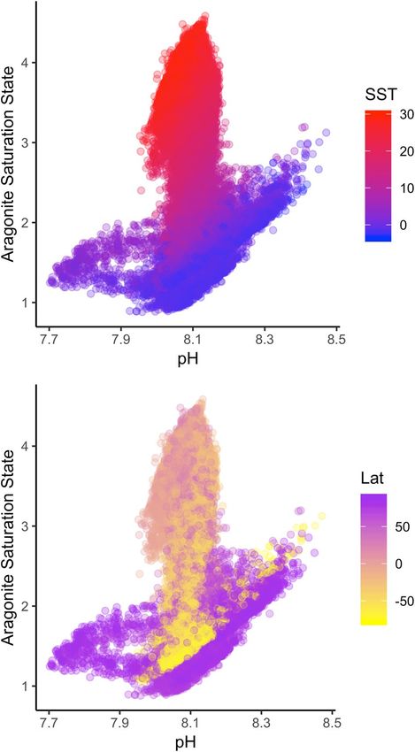
www.nature.com/scientificreports/
On the other hand, saturation state is the ratio of the ionic product, [ Ca2+][CO32−], to its saturated value. As satu-
ration state decreases, shell development becomes increasingly constrained by kinetics and energetics27, although
the specifics depend on the species. In marine bivalves, larval shell development and growth are dependent on
seawater saturation state, and not on carbon dioxide partial pressure or pH28. Note that because saturation state
increases slightly with temperature while pH decreases quickly with temperature, saturation states do not scale
linearly with pH and each of these variables represent different aspects of ocean climate3.
Data for this analysis was created by combining a recent observational carbon dioxide data product, the 6th
version of the Surface Ocean CO2 Atlas (SOCAT, 1991–2018, ~ 23 million observations), with a robust Earth
System Model29 to provide temporal trends at individual locations of the global ocean surface for aragonite satu-
ration state, SST, and pH from 1800–2100. Using these observation/model hybrid ensembles, we calculated the
degree of global novelty or d isappearance30 among the pre-industrial early nineteenth century (reconstructed),
the late twentieth century, and twenty-first century projections under different emissions scenarios. We compared
the nineteenth century pre-industrial reconstructed climate to the late twentieth century climate, and the late
twentieth century climate to the late twenty-first century climate for emissions scenarios RCP 4.5 (“stabilization”
emission response scenario where emissions peak in 2050, followed by slowed increase) and RCP 8.5 (worst case
“business as usual” scenario where emissions peak in 2100, followed by slowed increase). Over a decade of CO2
emissions since 2005 show that the RCP 2.6 scenario is too low to adequately represent the future atmosphere
CO2 level31–33. Consequently, the RCP 4.5 and RCP 8.5 scenarios are now the plausible low-end and high-end
concentration pathways.
Overview of metrics that reflect climate risk. We estimate the degree of global novelty or disappear-
ance using the Mahalanobian dissimilarity metrics developed by Mahony et al.30. These metrics are an improve-
ment over the standardized Euclidean d istance7 because the latter is susceptible to variance inflation due to
correlations in the raw variables and does not account for the effect of the number of variables on the statistical
meaning of distance. Following Mahony et al.30, we estimated two metrics that reflect climatic risk: (i) Mahalano-
bis distance (MD) (a multivariate distance) between a single gridpoint at one point in time and its closest analog
in the global baseline pool from another timepoint, and (ii) the transformation of MD into a standardized met-
ric called sigma dissimilarity (σD) that can be interpreted as the number of standard deviations of interannual
climate variability (ICV) at the focal station (see Table 1, definitions). The global climate baseline data includes
climate normals from widespread geographic locations in the hemisphere of the focal station (e.g., northern
or southern hemisphere) at a specific point of time. Following the framework outlined by Mahony et al.30, we
interpret 2–4σD to represent a moderate degree of global novelty/disappearance (corresponding to the 95th
percentile of the baseline) and greater than 4σD to represent an extreme degree of global novelty/disappearance
(corresponding to the 99.994th percentile of the baseline) (see Table 1, definitions). As a statistical measure of
the departure from historical variability, sigma dissimilarity provides an intrinsically meaningful metric of the
general ecological significance of climatic dissimilarities30.
We illustrate the calculation of sigma dissimilarity with hypothetical data in Fig. 1 for two hypothetical
climate variables, X1 and X2. In the left column of Fig. 1, the grey points represent the global climate baseline
data, which are shaded only for illustration. To calculate the degree of dissimilarity, σD, a principal components
analysis is performed on the global climate baseline data in the left column of Fig. 1 and standardized by the
multivariate interannual climate variability (ICV, magenta circles in Fig. 1) experienced at the focal station (blue
point in Fig. 1), resulting in the transformed data in the right column of Fig. 1 (see Table 1 for definitions). The
different shadings of grey in the global climate data are only used to help to visualize this transformation. In
this standardized principal components space, the degree of dissimilarity is then calculated as the number of
standard deviations between the climate normal at the focal station (blue point in Fig. 1) and the climate normal
of its nearest neighbor (e.g., closest analog) in the global climate baseline data (green diamond in Fig. 1). Via
the standardization, the degree of dissimilarity calculation incorporates the amount of ICV for the focal station.
Figure 1 illustrates the calculation for the degree of global novelty for a future climate projection at a focal
station compared to a present-day climate. A novel climate at a focal station occurs when a future climate normal
at that location does not currently exist in the present-day baseline of climate normals from geographic locations
across the same hemisphere (global climate baseline data, grey points in Fig. 1) and is projected to be outside
that historically experienced (e.g., the ICV) at the focal station. After transformation of the raw data (Fig. 1 left
column, for hypothetical environmental variables X1 and X2) with principal components and standardization by
the ICV (resulting in the data in Fig. 1 right column, arrows show how the loadings of environmental variables
X1 and X2 in PC space depend on the ICV), the degree of global novelty, σD-Novelty, is an estimate of the number
of standard deviations between the future climate normal at the focal station (blue point) and the climate normal
of its nearest neighbor (green diamond) in the present-day global climate baseline data (grey points, which are
shaded only to help visualize the standardization)30. In the principal components space (right side of Fig. 1),
the nearest neighbor (green diamond in Fig. 1) is the geographical location in the global baseline climate data
whose present-day climate normal is most similar to that of the focal station’s future projected climate normal
(e.g., closest analog).
In comparing Fig. 1A,B, the future climate predicted for the focal station (blue dot) and the nearest neighbor
(green diamond) is the same for both examples, but the ICV (magenta points) historically experienced at the
focal station is low (in A) or high (in B). When the focal geographical location experiences low ICV, the degree
of global novelty (σD-Novelty) to its nearest neighbor is large (Fig. 1A). When the focal geographical location expe-
riences high ICV, the degree of global novelty (σD-Novelty) is low (Fig. 1B). Thus, when all else is equal, σD varies
inversely with ICV. This is intuitive in the sense that a site that experiences a lot of climate variability would not
be expected to be as negatively impacted by climate change as a site that experiences less climate variability.
Scientific Reports | (2021) 11:15535 | https://doi.org/10.1038/s41598-021-94872-4 3
Vol.:(0123456789)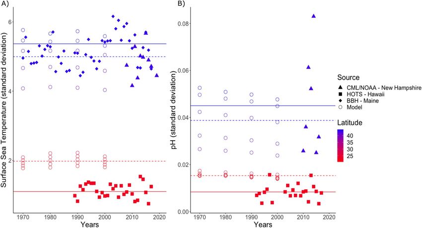
www.nature.com/scientificreports/

                                            Figure 1.  Illustration of climate novelty calculations. Hypothetical data for two focal geographic locations
                                            whose future climate normal (blue point, a novel climate in this case) is being compared to a global baseline of
                                            present-day climate normals (grey dots). The raw data (left column, for hypothetical environmental variables
                                            X1 and X2) is subject to a principal components analysis and then standardized by the multivariate interannual
                                            climate variability (ICV, pink circles) at the focal station, which results in the standardized data in the right
                                            column (arrows show how the loadings of environmental variables X1 and X2 in PC space depend on the ICV
                                            at the focal location). In the standardized PC space (right column), the degree of novelty (σD-Novelty) is calculated
                                            as the number of standard deviations between the climate projection at the focal station (blue point) and its
                                            nearest neighbor (green diamond) in the present-day global climate baseline data (grey points, which are
                                            shaded only to help visualize the standardization). (A) The novelty calculation for the future climate at a focal
                                            location that experiences low ICV is calculated to be extremely dissimilar to the global baseline. (B) The novelty
                                            calculation for the future climate at a focal location that is projected to be the same mean future climate as A,
                                            but experiences higher ICV, is calculated to have low dissimilarity to the global baseline. Note how the different
                                            degrees of ICV for X1 and X2 affect the data transformation into PC space. The degree of disappearance
                                            (σD-Disappearance) for a focal station is analogous to the grey points representing the global baseline for possible
                                            future climates, and the blue point representing today’s climate at the focal station. For further explanation see
                                            “Overview of metrics that reflect climate risk" section in the main text.

                                                Figure 1 can also be used to illustrate the degree of climate disappearance. A disappearing climate at a focal
                                            station is one that exists in the present-day, but is projected to no longer exist in the global baseline of future-time
                                            climates from widespread geographic locations. The degree of global disappearance (σD-Disappearance) for a focal
                                            geographic location is analogous to the grey points representing the global baseline data for projected future
                                            climate normals and the blue point representing today’s climate normal at the focal station. The magenta points
                                            still represent the ICV at the focal station, which is assumed to be constant through time. The σD-Disappearance is
                                            based on the number of standard deviations between the current climate normal at the focal station (blue point)
                                            and the climate normal for its nearest neighbor in the future-time climate (green diamond).

          Scientific Reports |   (2021) 11:15535 |                https://doi.org/10.1038/s41598-021-94872-4                                                      4

Vol:.(1234567890)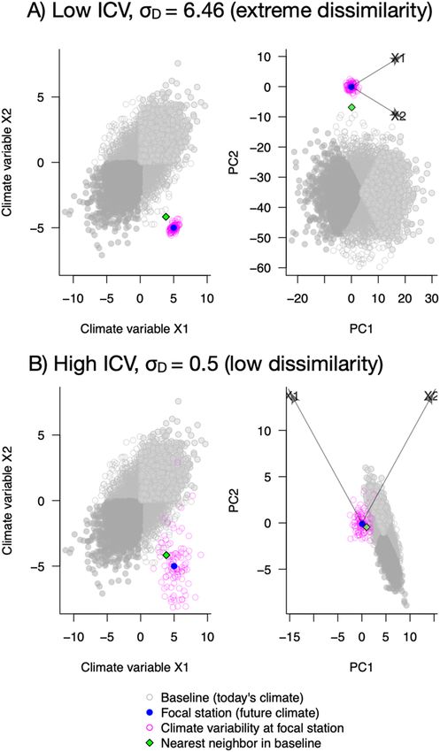
www.nature.com/scientificreports/
Figure 2. Distribution of pH versus aragonite saturation state in the global ocean. The points are colored by sea
surface temperature (SST, top) or latitude (Lat, bottom).
Results
Overview of model data. The model data has been previously p ublished3, so here we only briefly sum-
marize the patterns that are helpful in interpreting the multivariate analysis of global novelty and disappearance.
The relationship between saturation state, temperature, and pH in the present-day sea surface is shown in Fig. 2.
Because saturation state decreases with temperature, it does not scale linearly with pH and each of these vari-
ables represent different aspects of ocean climate. The local interannual climate variability that is used in the
standardization for the degree of global novelty/disappearance calculations is typically lowest for all variables
at the equator (Fig. 3). The temperate zones in the northern hemisphere typically have a more variable local
ICV than temperate zones in the southern hemisphere, and the Arctic experiences lower saturation states and
warmer conditions than Antarctic (Fig. 3).
Between 1800 and 2000, the shift in the individual climate variables as a function of latitude shows a slight
temperature increase at the equator and an ocean-wide slight drop in aragonite saturation state (Fig. 4 left col-
umn). Between 2000 and 2100, these shifts are projected to become larger under RCP 4.5 (Fig. 4 middle column)
and extreme under RCP 8.5 (Fig. 4 right column).
How these individual climate shifts correspond to the multivariate emergence of novel and disappearing
climates is visualized in Fig. 5 (for the northern hemisphere) and Fig. 6 (for the southern hemisphere). In the
northern hemisphere, the present-day undersaturated and low pH conditions in the Arctic are projected to
become more common at temperate latitudes under RCP 4.5 and RCP 8.5; note that for temperate latitudes these
conditions are unlikely to be globally novel because they are already common in the Arctic (Fig. 5 middle and
right columns, note overlap in 2000 and 2100 envelopes at low SST). In the southern hemisphere under RCP
8.5 projections, there is almost no overlap between current and projected climate envelopes across all latitudes
Scientific Reports | (2021) 11:15535 | https://doi.org/10.1038/s41598-021-94872-4 5
Vol.:(0123456789)www.nature.com/scientificreports/
30
25
20
SST 15
10
5
0
−78.5 −37.5 0 37.5 78.5
4
Arag.
3
2
1
−78.5 −37.5 0 37.5 78.5
8.5
8.4
8.3
8.2
pH
8.1
8.0
7.9
7.8
−78.5 −37.5 0 37.5 78.5
Latitude
Figure 3. Interannual climate variability as a function of latitude. Boxplots of the interannual climate variability
(ICV) used for the degree of climate novelty/disappearance as a function of latitude. The green area represents
the 0.25 and 0.75 quantiles (outliers were excluded). SST sea surface temperature, Arag aragonite saturation
state.
(Fig. 6 right column). While these figures are useful for comparing climate envelopes, note that they do not give
much insight into the degree of global novelty for a specific location, because that degree depends on the amount
of historical ICV at that location.
Degree of global novelty and disappearance between 1800 and 2000. Compared to 2000, 12.4%
of the modeled 1800 gridpoints had moderate degree of global disappearance and 0% had an extreme degree
of global disappearance (Table 2, Fig. 7A for MD-Disappearance and Fig. 8A for σD-Disappearance). Similarly, since 1800,
3.7% of the gridpoints from 2000 had a moderate degree of global novelty and 0% had an extreme degree of
global novelty (Table 3, Fig. 7B for MD-Novelty and Fig. 8B for σD-Novelty). Current globally disappearing climates are
trending in the Indian Ocean, the southwest Pacific, and tropical Atlantic (Fig. 7A), whereas current globally
novel climates are emerging in the equatorial Pacific (Fig. 7B). The relatively small climate shift since 1800 can be
visualized by the substantial overlap between the 1800 and 2000 climate envelopes for temperature and aragonite
saturation state and temperature and pH (Figs. 4, 5, 6).
Degree of global novelty and disappearance between 2000 and 2100. A substantial proportion
of the sea surface is projected to experience a moderate-to-extreme degree of global disappearance between 2000
and 2100 under RCP 4.5 and RCP 8.5. By 2100, between 35.6% (RCP 4.5) and 95% (RCP 8.5) of the sea surface
is predicted to experience an extreme degree of global disappearance (Table 2, Fig. 7C,E for MD-Disappearance and
Fig. 8C,E for σD-Disapperance). Locations with climates that are projected to experience the most extreme degree of
global disappearance are primarily located in the tropics and the temperate region of the southern hemisphere
(Figs. 7C,E and 8C,E), and become more widespread under RCP 8.5 (Fig. 8E).
A substantial proportion of the sea surface is also projected to experience a moderate-to-extreme degree of
global novelty between 2000 and 2100 under RCP 4.5 and RCP 8.5. By 2100, between 10.3% (RCP 4.5) and 81.9%
(RCP 8.5) of the sea surface is predicted to experience an extreme degree of global novelty (Table 3, Fig. 7D,F
Scientific Reports | (2021) 11:15535 | https://doi.org/10.1038/s41598-021-94872-4 6
Vol:.(1234567890)www.nature.com/scientificreports/
A) 1800 vs. 2000 SST B) 2000 vs. 2100 RCP 4.5 SST C) 2000 vs. 2100 RCP 8.5 SST
30 30 30
20 20 20
SST
SST
SST
10 10 10
0 0 0
−50 0 50 −50 0 50 −50 0 50
D) 1800 vs 2000 Arag E) 2000 vs. 2100 RCP 4.5 Arag F) 2000 vs. 2100 RCP 8.5 Arag
5.0 5.0 5.0
Year
4.0 4.0 4.0 1800
Arag
Arag
Arag
3.0 3.0 3.0 2000
2.0 2.0 2.0 2100 RCP 4.5
1.0 1.0 1.0 2100 RCP 8.5
0.0 0.0 0.0
−50 0 50 −50 0 50 −50 0 50
G) 1800 vs 2000 pH H) 2000 vs. 2100 RCP 4.5 pH I) 2000 vs. 2100 RCP 8.5 pH
8.5 8.5 8.5
8.0 8.0 8.0
pH
pH
pH
7.5 7.5 7.5
−50 0 50 −50 0 50 −50 0 50
Lat Lat Lat
Figure 4. Shifts in climate variables as a function of latitude. Univariate climate change for sea surface
temperature (SST, top row), aragonite saturation state (Arag, middle row), and pH (bottom row), as a function
of latitude for different century comparisons. The specific comparison is described in the title of each panel.
for MD-Disappearance and Fig. 8D,F for σD-Disapperance). Locations with climates that are projected to experience the
most extreme degree of global novelty are primarily located near the equator, in the Arctic, and in the sub-polar
region of the southern hemisphere (Figs. 7D,F and 8D,F), and become more widespread under RCP 8.5 (Fig. 8F).
The non-intuitive result that a larger proportion of sea surface climate will have a more extreme degree of
global disappearance than degree of global novelty is caused by the way the climate envelope shifts in the northern
hemisphere. A high density area of the temperature-pH envelope in 2000 does not overlap with the temperature-
pH envelope in 2100 (e.g., the former would have a high degree of global disappearance). However, a high density
area of the temperature-pH envelope in 2100 overlaps with some relatively rare locations in 2000 that have low
temperature and low pH (thus the lower degree of global novelty). Consequently, the multivariate distance from
a point at the end of the twentieth century to its nearest analog at the end of the twenty-first century (degree
of global disappearance) is more often larger than the multivariate distance from a point at the end of the 21th
century to its nearest analog at the end of the twentieth century (degree of global novelty).
Comparing model ICV with real data. If ICV is underestimated in our dataset, then the predictions for
MD and σD shown in Figs. 7 and 8 are overestimated. In comparing projections from the model to measured
values from long-term ocean monitoring time series, we found that variation in temporal field station measure-
ments of both SST and pH was lower in the tropics (as represented by Hawaiʻi) than at similar latitudes (between
20° N and 25° N) in the model (Fig. 9), indicating that our novelty projections for tropical regions (which are
already quite large) may be underestimated. Conversely, we found that variation in field station measurements of
both SST and pH was higher in the temperate zone (represented by Maine and New Hampshire) than at similar
latitudes (between 40° N and 45° N) in the model (Fig. 9), indicating that our novelty projections for this region
(which were among the lowest observed) may be overestimated. In summary, the qualitative prediction that
Scientific Reports | (2021) 11:15535 | https://doi.org/10.1038/s41598-021-94872-4 7
Vol.:(0123456789)www.nature.com/scientificreports/
A) 1800 vs 2000, N. Hem B) 2000 vs 2100 RCP 4.5, N. Hem C) 2000 vs 2100 RCP 8.5, N. Hem
Aragonite Saturation State
Aragonite Saturation State
Aragonite Saturation State
5.0 A) 1800 disappearing in 2000 5.0 2000 disappearing in 2100 RCP 4.5 5.0 2000 disappearing in 2100 RCP 8.5
4.0 4.0 4.0
3.0 3.0 3.0
2.0 2.0 2.0
Novel in 2000
1.0 1.0 1.0
Novel iin 2100 RCP 4.5
Year
Novel in 2100
2 RCP 8.5
0.0 0.0 0.0
0 10 20 30 0 10 20 30 0 10 20 30 1800
SST SST SST
2000
D) 1800 vs 2000, N. Hem E) 2000 vs 2100 RCP 4.5, N. Hem F) 2000 vs 2100 RCP 8.5, N. Hem
1800 disappearing in 2000 2000 disappearing in 2100 RCP 4.5 2000 disappearing in 2100 RCP 8.5
2100 RCP 4.5
8.5 8.5 8.5 2100 RCP 8.5
8.0 8.0 8.0
pH
pH
pH
Novel in 2000 Novel in 2100 RCP 4.5
N
7.5 7.5 7.5 Novel in 2100 RCP 8.5
N
0 10 20 30 0 10 20 30 0 10 20 30
SST SST SST
Figure 5. Shifts in climate envelopes for the northern hemisphere. We compared the distribution of sea surface
climate normals between different centuries in the northern hemisphere. Aragonite saturation state (top row)
or pH (bottom row) are plotted against sea surface temperature (SST). For specific comparisons see the titles
in each panel. When aragonite saturation state falls below 1.0 (horizontal dotted line), the calcium carbonate
polymorph that some marine animals use to make their shells will dissolve into seawater.
A) 1800 vs 2000, S. Hem B) 2000 vs 2100 RCP 4.5, S. Hem C) 2000 vs 2100 RCP 8.5, S. Hem
Aragonite Saturation State
Aragonite Saturation State
Aragonite Saturation State
5.0 A) 1800 disappearing in 2000 5.0 2000 disappearing in 2100 RCP 4.5 5.0 2000 disappearing in 2100 RCP 8.5
4.0 4.0 4.0
3.0 3.0 3.0
2.0 2.0 2.0
Novel in 2000
1.0 1.0 1.0
Novel iin 2100 RCP 4.5
Year
Novel in 2100
1 RCP 8.5
0.0 0.0 0.0
0 10 20 30 0 10 20 30 0 10 20 30 1800
SST SST SST
2000
D) 1800 vs 2000, S. Hem E) 2000 vs 2100 RCP 4.5, S. Hem F) 2000 vs 2100 RCP 8.5, S. Hem
1800 disappearing in 2000 2000 disappearing in 2100 RCP 4.5 2000 disappearing in 2100 RCP 8.5
2100 RCP 4.5
8.5 8.5 8.5 2100 RCP 8.5
8.0 8.0 8.0
pH
pH
pH
Novel in 2000
N Novel in 2100 RCP 4.5
N
7.5 7.5 7.5 Novel in 2100 RCP 8.5
N
0 10 20 30 0 10 20 30 0 10 20 30
SST SST SST
Figure 6. Shifts in climate envelopes for the southern hemisphere. We compared the distribution of sea surface
climate normals between different centuries in the southern hemisphere. Sea surface temperature (SST) is
plotted against aragonite saturation state (top row) or pH (bottom row). For specific comparisons see the titles
in each panel. When aragonite saturation state falls below 1.0 (horizontal dotted line), the calcium carbonate
polymorph that some marine animals use to make their shells will dissolve into seawater.
Scientific Reports | (2021) 11:15535 | https://doi.org/10.1038/s41598-021-94872-4 8
Vol:.(1234567890)www.nature.com/scientificreports/
Degree of global disappearance σD-Disappearance 1800–2000 (%) 2000–2100 RCP 4.5 (%) 2000–2100 RCP 8.5 (%)
Low (σD < 2) 87.6 30.2 1.5
Moderate (2 < σD < 4) 12.4 34.2 3.5
High (σD > 4) 0 35.6 95
Table 2. Percent of ocean surface estimated to experience different degrees of global disappearance.
Figure 7. Map of climate risk based on Mahalanobis distance. A map of the multivariate distance between the
climate normal for each gridpoint at one point in time and its closest analog in the global climate baseline data
at another point in time (Mahalanobis distance, MD). The MD,Disappearance is the multivariate distance between the
climate normal of a gridpoint at an earlier time to its closest analog in the global baseline climate normals at
a later time (left column). The MD,Novelty is the multivariate distance between the climate normal of a gridpoint
at a later time to its closest analog in the global baseline climate normals at an earlier time (right column). For
specific comparisons see the titles within each panel.
Scientific Reports | (2021) 11:15535 | https://doi.org/10.1038/s41598-021-94872-4 9
Vol.:(0123456789)www.nature.com/scientificreports/
Figure 8. Map of climate risk based on sigma dissimilarity. The degree of global disappearance or novelty for
the global ocean. Sigma dissimilarity (σD) represents the number of standard deviations of the local interannual
climatic variability (ICV) at a gridpoint at one point in time from its closest analog in a global pool of data at
a different point in time. The degree of global disappearance (σD-Disappearance) is the dissimilarity between the
climate normal of a gridpoint at an earlier time to its closest analog in the global baseline climate normals
at a later time (left column). The degree of global novelty (σD-Novelty) is the dissimilarity between the climate
normal of a gridpoint at a later time to its closest analog in the global baseline climate normals at an earlier
time (left column). For specific comparisons see the titles within each panel. The largest σD that could be
calculated with decimal precision was 8.29σ. Following30, a moderate degree of novelty or disappearance is
given by 2 < σD < (corresponding to the the 95th percentile of local ICV) and an extreme degree is given by σD > 4
(corresponding to the the 99.994th percentile of local ICV).
Degree of global novelty σD-Novelty 1800–2000 (%) 2000–2100 RCP 4.5 (%) 2000–2100 RCP 8.5 (%)
Low (σD < 2) 96.3 47.6 11.4
Moderate (2 < σD < 4) 3.7 42.1 6.7
High (σD > 4) 0 10.3 81.9
Table 3. Percent of ocean surface estimated to experience different degrees of global novelty.
Scientific Reports | (2021) 11:15535 | https://doi.org/10.1038/s41598-021-94872-4 10
Vol:.(1234567890)www.nature.com/scientificreports/
Figure 9. Comparison of ICV for observational versus model data. We compared long-term ocean field site
measurement standard deviations in sea surface temperature (A) and pH (B) to model standard deviations at
representative latitudes and longitudes. The solid lines represent the average annual standard deviation of the
field measured time series data, while the dotted line represents the average standard deviation of the model in
the same region. The observational data included the tropical Hawaii Ocean Time-series (HOTS), the temperate
North Atlantic datasets from the University of New Hampshire Coastal Marine Laboratory and the National
Oceanic and Atmospheric Administration mooring NH_70W_43N (CML/NOAA), and Boothbay Harbor,
Maine (BBH).
equatorial regions will experience an extreme degree of global novelty and northern temperate regions will not
experience globally novel conditions is robust given the direction of the slight biases in the ICV.
Discussion
Our analysis did not predict that any modeled gridpoints on the ocean surface have experienced an extreme
degree of global disappearance or novelty between 1800 and 2000. However, between 2000 and 2100 under
Representative Concentrations Pathway (RCP 4.5 or 8.5) projections, our analysis predicted that a substantial
proportion of the sea surface may experience an extreme degree of global novelty and disappearance relative to
the global climate baseline data. The upward estimates in our analysis are larger than those projected for global
novel and disappearing climates on land7, and are due in part to the ocean surface environment being two to
three orders of magnitude less variable than that on l and34. Under both RCP 4.5 and RCP 8.5, the more extreme
degree of global novelty near the equator and in the sub-Antarctic is driven in part by the lower interannual
climatic variability (ICV) at these locations. In contrast, the low degree of global novelty in northern temperate
regions stems in part from the higher ICV at those latitudes.
In this study we estimated the degree of multivariate novelty of future climates and disappearance of extant
climates relative to global climate baseline data for the sea surface, which complements previous studies for the
global ocean based on local rates of climate change15,16. The local versus global metrics provide important, and
different, information about the vulnerability of populations to climate change. Local climate change at a specific
location, relative to the historical variability at that location, may reflect the extent to which the species composi-
tion will shift as species track shifting climate envelopes with dispersal. The degree of global climate novelty at a
location, however, may indicate how stressful novel conditions will be for all species. In contrast, the degree of
global climate disappearance for a location may represent how hard it might be for species who are well adapted
to the climate at that location to find a similar climate in the future.
While dispersal limitations greatly increase the risk that species will experience the loss of extant climates or
the occurrence of novel climates7, the high dispersal potential of marine organisms with a planktonic larval stage
has been discussed as a trait that will allow them to keep pace with climate c hange15. Recent studies have found
that marine species are able to track shifting c limates10,11. Our study shows that the majority of these climate shifts
are not novel (e.g., have an analog) since the early nineteenth century. In other words, although some climate
variables, such as pH, have already emerged beyond historical baseline for a particular location15, our study shows
these climates are not novel from a global perspective and may facilitate tracking via range shifts. However, if a
majority of the ocean surface climate disappears and is replaced by novel climates with no recent analog by the
end of the twenty-first century, the optimal environment for many species may not exist and dispersal will not
Scientific Reports | (2021) 11:15535 | https://doi.org/10.1038/s41598-021-94872-4 11
Vol.:(0123456789)www.nature.com/scientificreports/
help these species keep pace with environmental change. Instead, species may need to keep pace via evolutionary
adaptation, plasticity and acclimatization, and/or epigenetic p rocesses35.
Evidence for adaptive capacity is emerging, although examples are still few. Phytoplankton have been shown
to evolve rapidly in response to increased pCO213, due in part to their short generation times and large popula-
tion sizes. The concerns remain, however, that adaptive variation for high pCO2 is limited in most s pecies36, that
high pCO2 can diminish the heritability of larval traits37, that marine species live close to their upper thermal
limits38, and that the unprecedented rate of change will be too fast relative to the long life span of many marine
species for adaptive evolution to occur before their lineages go e xtinct39. Yet, a growing number of studies have
found transgenerational plasticity of marine invertebrates and vertebrates in response to increased temperature
or pCO240,41, suggesting that non-genetic or epigenetic processes could play a major role in acclimatization—
although there are many knowledge gaps in the molecular mechanisms that underlie such p rocesses42.
The degree of global novelty or disappearance for a specific location is relative to the amount of variability
historically experienced at a location. We found that the model data tended to have lower ICV than time series
data for high latitudes, and higher ICV than time series data for low latitudes, indicating that our estimates of
novelty may be overestimated for high latitudes (which are already the lowest novelty) and underestimated for
low latitudes (which are already the highest novelty). Therefore, the main conclusion—that the equator and
sub-Antarctic regions will experience the highest degree of global novelty and northern temperate regions the
lowest degree of global novelty—is robust to the direction of bias we observed in the ICV. Note, however, that
our analysis did not include coastal areas, which are known to experience large fluctuations in temperature and
carbonate chemistry due to upwelling processes and freshwater i nput43,44. Including coastal areas in this analysis
was not possible due to the paucity of data, but would be an important avenue for future research.
Our projections may be conservative because there are other important aspects of seawater chemistry, food
availability, and ocean dynamics that will be altered by climate change but were not considered by our model. For
example, enhanced stratification caused by warming temperatures can have a range of indirect effects, including
reduced nutrient supply to phytoplankton at low latitudes, but a more favorable light regime for these organisms
at high latitudes45,46. Primary productivity may also be altered in coastal areas where productivity is driven by
the seasonal upwelling of deep, nutrient-rich water. Climate change is altering the intensity, timing and spatial
structure of upwelling dynamics, thus reshaping patterns of primary productivity47–50. Warming also reduces
the solubility of oxygen, and hypoxic conditions have been shown to have negative effects on many marine
organisms51. Moreover, warming drives sea ice melt and systematic freshening of polar a reas52.
Including multiple stressors into calculations of MD and σD is an important avenue for future research. In our
analysis, reconstructed and projected carbonate chemistry for the global ocean was based on the GFDL-ESM2M
model that is often considered as the most reliable model for the carbonate parameters (Dunne et al. 2012, 2013).
Other models with different variables (e.g. sea ice, salinity, dissolved oxygen, nutrients, etc.) could be analysed in
the same way and this would allow an estimate of the uncertainty in the results. The sensitivity of the results to the
choice of model is an important next step towards producing more robust estimates of novelty and disappearance.
If the projections of climate novelty and disappearance reported here are accurate, the cascading effects on
marine ecosystems and communities could be substantial. Areas such as the IndoPacific, which are projected
to experience the most extreme degree of climate novelty and disappearance, are critical hot spots for endemic
biodiversity and coral reefs53–55. Coral reefs are particularly vulnerable to bleaching of their zooxanthellae symbi-
onts, which can result from minor increases in temperature50. In these areas, elevated risks of ecological surprises,
including extinction, are likely.
Shifting climate niches only represent one aspect of the ecological risks associated with climate change. Modi-
fied energy flows and biogeochemical cycles, multiple stressors, shifts in phenology, climate-mediated invasions,
climate-driven disease outbreaks, and asynchronies between prey availability and predator demand are some of
the other processes that will contribute to shifting ecosystem distributions and the services that they provide to
society50,56,57. Species will vary in their ability to keep up with multivariate environmental transitions into no-
analog climates, which will promote the formation of no-analog species assemblages and present many ecological
surprises. Highly novel marine ecosystems will challenge the predictive ability of eco-evolutionary models and
present many challenges to the preservation of marine biodiversity over the next century.
Methods
Global ocean reconstructed and projected data. Seawater carbonate data for pH and aragonite sat-
uration state calculation in this study were extracted from the 6th version of the Surface Ocean CO2 Atlas
(SOCATv6, 1991–2018, ~ 23 million observations) at a spatial resolution of 1 × 1 degree58. Data without quality
control flags of A or B (uncertainty of fugacity of carbon dioxide, fCO2 < 2 µatm) were omitted. Silicate and phos-
phate values for all SOCATv6 stations were extracted from the gridded GLODAPv2 c limatologies59. Total alka-
linity (TA) was then calculated with the updated Locally Interpolated Alkalinity Regression (LIARv2) method60.
pH on the total hydrogen scale ( pHT) and aragonite saturation state were calculated from in-situ temperature,
salinity, hydrostatic pressure, dissolved inorganic carbon (DIC) concentration, TA, silicate and phosphate. Dis-
sociation constants were taken from the literature for carbonic acid61, bisulfate (HSO4−)62, and hydrofluoric acid
(HF)63. Total borate concentration equations were the same as reported by Uppström64. A MATLAB v ersion65 of
the CO2SYS program66 was used for analysis. Uncertainties of the methods using the CO2SYS errors program67
are estimated to be 0.01 for pH and 0.13 for aragonite saturation state, assuming uncertainties for SST, salinity,
TA, and DIC of 0.01, 0.02, 6 µmol kg−1 and 4 µmol kg−1, respectively.
The calculated p HT and aragonite were then adjusted from their sampling year to 2000 assuming that: (a) sea
surface pCO2 increases at the same rate as atmospheric mole fraction of carbon dioxide ( xCO2), as documented
by the IPCC Fifth Assessment Report 5 (AR5)68, (b) SST increases at the rate described by NOAA’s Extended
Scientific Reports | (2021) 11:15535 | https://doi.org/10.1038/s41598-021-94872-4 12
Vol:.(1234567890)www.nature.com/scientificreports/
Reconstructed Sea Surface Temperature (ERSST) v 569, and (c) salinity and TA remain constant. Surface pHT and
Revelle Factor were further adjusted from their sampling month to all 12 months of 2000 assuming that: (a) sea
surface pCO2 follows the same annual cycle as documented by the LDEO database70, (b) sea surface temperature
(SST) in all months of 2000 can be approximated by the 1995–2004 average monthly SST climatology from the
World Ocean A tlas71 and (c) salinity and TA remain constant.
Surface ocean p HT and aragonite saturation state in all 12 months for all decades from 1770 to 2100 under
the IPCC scenarios (RCP 4.5 and RCP 8.5) were reconstructed or projected assuming that sea surface pCO2 and
SST increase at the rate simulated by the GFDL-ESM2M model run with these pathways2,29. Spatial mapping was
conducted using a Matlab version (Divand Software) of the Data-Interpolating Variational Analysis (DIVA)72.
For more detail, please refer to Jiang et al.3.
Estimating global climate novelty or disappearance. For each location, the metrics we estimate are
based on dissimilarity between the projected multivariate (past or future/projected) climate change at a given
location and its nearest analog in a global set of “baseline” data. To estimate the range of possible degrees of nov-
elty or disappearance, we compared the predictions for a global baseline and a hemisphere-restricted baseline
(e.g., northern or southern hemisphere). An important feature of our calculations is that they (i) are performed
in multivariate space, and (ii) take into account the interannual climatic variability (ICV) at that location. For all
analyses, climate normals were calculated based on 40-year means of each climate variable and ICV was based
on model data for 1965–2004 (see Table 1 for definitions). Because the ICV did not change substantially through
time in the model data, our results were not sensitive to the span of years chosen to represent the ICV.
Aragonite saturation state was log10-transformed because it was a ratio variable: it is limited at zero and
proportional changes are meaningful (C. R. Mahoney, pers. comm.). This transformation makes the difference
between 1 and 2 the same significance as the difference between 0.5 and 1 (doubling vs. halving, i.e., proportional
scaling). In practice, temperature doesn’t need to be log-transformed because it doesn’t vary across orders of
magnitude, and in our case pH is already a log-scaled variable. Nevertheless, our analysis was not sensitive to
whether or not aragonite saturation state was log-transformed.
The degree of global novelty is calculated by comparing a later climate normal for each ocean gridpoint to all
earlier climate normals for the global baseline data. We performed three planned comparisons for the degree of
climate novelty as measured by MD-novelty and σD-novelty (note we use the reference period 1965–2004 ICV for all
analyses): (i) novelty of the late twentieth century ocean surface (1965–2004) compared to pre-industrial early
nineteenth century (1795–1834) reconstructed climate; (ii) novelty of the late twenty-first century climate under
RCP 4.5 (2065–2104) compared to late twentieth century; and (iii) novelty of the late twenty-first century climate
under RCP 8.5 (2065–2104) compared to late twentieth century.
Conversely, the degree of global disappearance is calculated by comparing an earlier climate normal for each
ocean gridpoint to a later pool of climate normals for the global baseline data. High values indicate places where
climates may disappear; i.e., they have no close counterpart anywhere in the later timepoint. We performed three
planned comparisons for the degree of climate disappearance as measured by MD-disapperance and σD-disappearance: (i)
disappearance of climates from early nineteenth century pre-industrial times (1795–1835 reconstructed climate)
in the late twentieth century ocean (1965–2005); (ii) disappearance of late twentieth century climates by the late
twenty-first century under RCP 4.5 (2065–2105); and (iii) disappearance of twentieth century climates by the
late twenty-first century under RCP 8.5 (2065–2105).
Values of σD higher than ~ 8 were difficult to estimate due to the high decimal precision required to estimate
probability in the extreme tail of the chi distribution; in these cases σD was set to a value of 8.29 σ (the maximum
value that could be calculated given decimal precision). We created maps of MD and σD in Matlab R2021 Version
(code available in repo).
Comparing ICV between model projections and real data. Because of the sensitivity of the degree
of global novelty/disappearance calculations to the ICV (see An overview of global climate novelty and disappear-
ance calculations), we wanted to ensure the ICV that we used from the model data were similar to those observed
in long-term ocean time series. We were particularly concerned whether ICV might be underestimated in the
model data, because that would bias our estimates of MD and σD upwards. To explore whether ICV in the model
projections were lower or greater than that observed in long-term ocean time series, and to address some of
the limitations due to the coarse grid of global models, we compared SST and pH standard deviations from the
model to those from long-term ocean monitoring time series in the tropical and temperate zones.
The model output is the predicted climate variable for that ocean gridpoint for each month, and it is calculated
every decade. The standard deviation of the modeled data is based on the monthly data for each year that data is
available. The observational data, however, is collected continuously across an entire year. The standard deviation
of the observational data is based on this continuous data for each year that data is available.
Real measurements of SST and surface pH were downloaded from Hawaii Ocean Time Series73, and from
the University of New Hampshire Coastal Marine L aboratory74; SST was also acquired from Boothbay H arbor75;
and additional pH measurements from the National Oceanic and Atmospheric Administration mooring
NH_70W_43N (NOAA)76. For regional comparisons, the tropical central Pacific (HOTS) dataset was compared
to model data for values between latitude 20° N and 25° N, and longitude 160° E and 130° W, and the temperate
North Atlantic (UNH_CML, BBH & NOAA) data were compared to model data for values between latitude
40° N and 45° N, and longitudes 40° W and 70° W. For the time series data, years in which measurements were
not sampled continuously across both winter and summer months were omitted. Yearly standard deviations of
both SST and pH for the observational and model data were calculated and compared in R.
Scientific Reports | (2021) 11:15535 | https://doi.org/10.1038/s41598-021-94872-4 13
Vol.:(0123456789)www.nature.com/scientificreports/
Data availability
Code and data for reproducing the results can be found at the Dryad repository: Data from: Novel and disap-
pearing climates in the global surface ocean from 1800 to 2100 (doi:https://doi.org/10.5061/dryad.ht76hdrgb).
Received: 19 January 2021; Accepted: 13 July 2021
References
1. IPCC. Climate Change 2013: The Physical Science Basis. Working Group I Contribution to the Fifth Assessment Report of the Inter-
governmental Panel on Climate Change (Cambridge University Press, 2013).
2. Dunne, J. P. et al. GFDL’s ESM2 global coupled climate-carbon earth system models. Part II: Carbon system formulation and
baseline simulation characteristics. J. Clim. 26, 2247–2267 (2013).
3. Jiang, L.-Q., Carter, B. R., Feely, R. A., Lauvset, S. K. & Olsen, A. Surface ocean pH and buffer capacity: Past, present and future.
Nat. Sci. Rep. 9, 18624 (2019).
4. Caldeira, K. & Wickett, M. E. Oceanography: Anthropogenic carbon and ocean pH. Nature 425, 365–365 (2003).
5. Hoegh-Guldberg, O. et al. Coral reefs under rapid climate change and ocean acidification. Science 318, 1737–1742 (2007).
6. Hönisch, B. et al. The geological record of ocean acidification. Science 335, 1058–1063 (2012).
7. Williams, J. W., Jackson, S. T. & Kutzbach, J. E. Projected distributions of novel and disappearing climates by 2100 AD. Proc. Natl.
Acad. Sci. U. S. A. 104, 5738–5742 (2007).
8. Williams, J. W. & Jackson, S. T. Novel climates, no-analog communities, and ecological surprises. Front. Ecol. Environ. 5, 475–482
(2007).
9. Radeloff, V. C. et al. The rise of novelty in ecosystems. Ecol. Appl. 25, 2051–2068 (2015).
10. Sunday, J. M., Bates, A. E. & Dulvy, N. K. Thermal tolerance and the global redistribution of animals. Nat. Clim. Change 2, 686–690
(2012).
11. Pinsky, M. L., Worm, B., Fogarty, M. J., Sarmiento, J. L. & Levin, S. A. Marine taxa track local climate velocities. Science 341,
1239–1242 (2013).
12. Pinsky, M. L., Selden, R. L. & Kitchel, Z. J. Climate-driven shifts in marine species ranges: Scaling from organisms to communities.
Ann. Rev. Mar. Sci. 12, 153–179 (2020).
13. Bell, G. & Collins, S. Adaptation, extinction and global change. Evol. Appl. 1, 3–16 (2008).
14. Lancaster, L. T., Morrison, G. & Fitt, R. N. Life history trade-offs, the intensity of competition, and coexistence in novel and evolv-
ing communities under climate change. Philos. Trans. R. Soc. Lond. B Biol. Sci. 372, 20160046 (2017).
15. Henson, S. A. et al. Rapid emergence of climate change in environmental drivers of marine ecosystems. Nat. Commun. 8, 14682
(2017).
16. Bruno, J. F. et al. Climate change threatens the world’s marine protected areas. Nat. Clim. Change 8, 499–503 (2018).
17. Turk, D. et al. Time of emergence of surface ocean carbon dioxide trends in the North American coastal margins in support of
ocean acidification observing system design. Front. Mar. Sci. 6, 91 (2019).
18. Jiang, L.-Q. et al. Climatological distribution of aragonite saturation state in the global oceans. Global Biogeochem. Cycles 29,
1656–1673 (2015).
19. Orr, J. C. et al. Anthropogenic ocean acidification over the twenty-first century and its impact on calcifying organisms. Nature
437, 681–686 (2005).
20. Feely, R. A., Doney, S. C. & Cooley, S. R. Ocean acidification: Present conditions and future changes in a high-CO2 world. Ocean-
ography 22, 36–47 (2009).
21. Tittensor, D. P. et al. Global patterns and predictors of marine biodiversity across taxa. Nature 466, 1098–1101 (2010).
22. Allen, A. P., Brown, J. H. & Gillooly, J. F. Global biodiversity, biochemical kinetics, and the energetic-equivalence rule. Science 297,
1545–1548 (2002).
23. Donner, S. D. Coping with commitment: Projected thermal stress on coral reefs under different future scenarios. PLoS ONE 4,
e5712 (2009).
24. Walsh, P. J. & Louise Milligan, C. Coordination of metabolism and intracellular acid–base status: Ionic regulation and metabolic
consequences. Can. J. Zool. 67, 2994–3004 (1989).
25. Nilsson, G. E. et al. Near-future carbon dioxide levels alter fish behaviour by interfering with neurotransmitter function. Nat. Clim.
Change 2, 201–204 (2012).
26. Clark, T. D. et al. Ocean acidification does not impair the behaviour of coral reef fishes. Nature 577, 370–375 (2020).
27. Waldbusser, G. G. et al. A developmental and energetic basis linking larval oyster shell formation to acidification sensitivity.
Geophys. Res. Lett. 40, 2171–2176 (2013).
28. Waldbusser, G. G. et al. Saturation-state sensitivity of marine bivalve larvae to ocean acidification. Nat. Clim. Change 5, 273–280
(2015).
29. Dunne, J. P. et al. GFDL’s ESM2 global coupled climate-carbon earth system models. Part I: Physical formulation and baseline
simulation characteristics. J. Clim. 25, 6646–6665 (2012).
30. Mahony, C. R., Cannon, A. J., Wang, T. & Aitken, S. N. A closer look at novel climates: New methods and insights at continental
to landscape scales. Glob. Change Biol. https://doi.org/10.1111/gcb.13645 (2017).
31. Millar, R. J. et al. Emission budgets and pathways consistent with limiting warming to 1.5 °C. Nat. Geosci. 10, 741–747 (2017).
32. Sanderson, B. M., O’Neill, B. C. & Tebaldi, C. What would it take to achieve the Paris temperature targets?. Geophys. Res. Lett. 43,
7133–7142 (2016).
33. Friedlingstein, P. et al. Persistent growth of C O2 emissions and implications for reaching climate targets. Nat. Geosci. 7, 709–715
(2014).
34. Steele, J. H., Brink, K. H. & Scott, B. E. Comparison of marine and terrestrial ecosystems: Suggestions of an evolutionary perspec-
tive influenced by environmental variation. ICES J. Mar. Sci. 76, 50–59 (2019).
35. Munday, P. L., Warner, R. R., Monro, K., Pandolfi, J. M. & Marshall, D. J. Predicting evolutionary responses to climate change in
the sea. Ecol. Lett. 16, 1488–1500 (2013).
36. Kelly, M. W. & Hofmann, G. E. Adaptation and the physiology of ocean acidification. Funct. Ecol. 27, 980–990 (2013).
37. Sunday, J. M. et al. Evolution in an acidifying ocean. Trends Ecol. Evol. 29, 117–125 (2014).
38. Pinsky, M. L., Eikeset, A. M., McCauley, D. J., Payne, J. L. & Sunday, J. M. Greater vulnerability to warming of marine versus ter-
restrial ectotherms. Nature 569, 108–111 (2019).
39. Hoegh-Guldberg, O. Climate change, coral bleaching and the future of the world’s coral reefs. Mar. Freshw. Res. 50, 839–866 (1999).
40. Donelson, J. M., Salinas, S., Munday, P. L. & Shama, L. N. S. Transgenerational plasticity and climate change experiments: Where
do we go from here?. Glob. Change Biol. 24, 13–34 (2018).
41. Ross, P. M., Parker, L. & Byrne, M. Transgenerational responses of molluscs and echinoderms to changing ocean conditions. ICES
J. Mar. Sci. 73, 537–549 (2016).
42. Eirin-Lopez, J. M. & Putnam, H. M. Marine environmental epigenetics. Ann. Rev. Mar. Sci. 11, 335–368 (2019).
Scientific Reports | (2021) 11:15535 | https://doi.org/10.1038/s41598-021-94872-4 14
Vol:.(1234567890)You can also read