Mendeleev Documentation - Release 0.9.0 Lukasz Mentel - mendeleev's documentation
←
→
Page content transcription
If your browser does not render page correctly, please read the page content below
mendeleev Documentation
 Release 0.9.0

 Lukasz Mentel

 Jan 21, 2022
CONTENTS

1 Getting started 3
 1.1 Overview . . . . . . . . . . . . . . . . . . . . . . . . . . . . . . . . . . . . . . . . . . . . . . . . . 3
 1.2 Contributing . . . . . . . . . . . . . . . . . . . . . . . . . . . . . . . . . . . . . . . . . . . . . . . 3
 1.3 Citing . . . . . . . . . . . . . . . . . . . . . . . . . . . . . . . . . . . . . . . . . . . . . . . . . . . 3
 1.4 Related projects . . . . . . . . . . . . . . . . . . . . . . . . . . . . . . . . . . . . . . . . . . . . . 4
 1.5 Funding . . . . . . . . . . . . . . . . . . . . . . . . . . . . . . . . . . . . . . . . . . . . . . . . . . 4

2 Installation 5

3 Tutorials 7
 3.1 Quick start . . . . . . . . . . . . . . . . . . . . . . . . . . . . . . . . . . . . . . . . . . . . . . . . 7
 3.2 Bulk data access . . . . . . . . . . . . . . . . . . . . . . . . . . . . . . . . . . . . . . . . . . . . . 14
 3.3 Electronic configuration . . . . . . . . . . . . . . . . . . . . . . . . . . . . . . . . . . . . . . . . . 21
 3.4 Ions . . . . . . . . . . . . . . . . . . . . . . . . . . . . . . . . . . . . . . . . . . . . . . . . . . . . 23
 3.5 Visualizing custom periodic tables . . . . . . . . . . . . . . . . . . . . . . . . . . . . . . . . . . . . 25
 3.6 Advanced visulization tutorial . . . . . . . . . . . . . . . . . . . . . . . . . . . . . . . . . . . . . . 27
 3.7 Jupyter notebooks . . . . . . . . . . . . . . . . . . . . . . . . . . . . . . . . . . . . . . . . . . . . 30

4 Data 31
 4.1 Elements . . . . . . . . . . . . . . . . . . . . . . . . . . . . . . . . . . . . . . . . . . . . . . . . . 31
 4.2 Isotopes . . . . . . . . . . . . . . . . . . . . . . . . . . . . . . . . . . . . . . . . . . . . . . . . . . 35

5 Electronegativities 37
 5.1 Allen . . . . . . . . . . . . . . . . . . . . . . . . . . . . . . . . . . . . . . . . . . . . . . . . . . . 37
 5.2 Allred and Rochow . . . . . . . . . . . . . . . . . . . . . . . . . . . . . . . . . . . . . . . . . . . . 38
 5.3 Cottrell and Sutton . . . . . . . . . . . . . . . . . . . . . . . . . . . . . . . . . . . . . . . . . . . . 38
 5.4 Ghosh . . . . . . . . . . . . . . . . . . . . . . . . . . . . . . . . . . . . . . . . . . . . . . . . . . . 38
 5.5 Gordy . . . . . . . . . . . . . . . . . . . . . . . . . . . . . . . . . . . . . . . . . . . . . . . . . . . 39
 5.6 Li and Xue . . . . . . . . . . . . . . . . . . . . . . . . . . . . . . . . . . . . . . . . . . . . . . . . 39
 5.7 Martynov and Batsanov . . . . . . . . . . . . . . . . . . . . . . . . . . . . . . . . . . . . . . . . . 39
 5.8 Mulliken . . . . . . . . . . . . . . . . . . . . . . . . . . . . . . . . . . . . . . . . . . . . . . . . . 40
 5.9 Nagle . . . . . . . . . . . . . . . . . . . . . . . . . . . . . . . . . . . . . . . . . . . . . . . . . . . 40
 5.10 Pauling . . . . . . . . . . . . . . . . . . . . . . . . . . . . . . . . . . . . . . . . . . . . . . . . . . 40
 5.11 Sanderson . . . . . . . . . . . . . . . . . . . . . . . . . . . . . . . . . . . . . . . . . . . . . . . . 40
 5.12 Fetching all electronegativities . . . . . . . . . . . . . . . . . . . . . . . . . . . . . . . . . . . . . . 41

6 API Reference 43
 6.1 Accessing data . . . . . . . . . . . . . . . . . . . . . . . . . . . . . . . . . . . . . . . . . . . . . . 43
 6.2 Classes . . . . . . . . . . . . . . . . . . . . . . . . . . . . . . . . . . . . . . . . . . . . . . . . . . 45
 6.3 Modules . . . . . . . . . . . . . . . . . . . . . . . . . . . . . . . . . . . . . . . . . . . . . . . . . 54

 i
7 Bibliography 57

8 mendeleev Changelog 59
 8.1 v0.9.0 (24.09.2021) . . . . . . . . . . . . . . . . . . . . . . . . . . . . . . . . . . . . . . . . . . . 59
 8.2 v0.8.0 (22.08.2021) . . . . . . . . . . . . . . . . . . . . . . . . . . . . . . . . . . . . . . . . . . . 59
 8.3 v0.7.0 (20.03.2021) . . . . . . . . . . . . . . . . . . . . . . . . . . . . . . . . . . . . . . . . . . . 59
 8.4 v0.6.1 (03.11.2020) . . . . . . . . . . . . . . . . . . . . . . . . . . . . . . . . . . . . . . . . . . . 60
 8.5 v0.6.0 (10.04.2020) . . . . . . . . . . . . . . . . . . . . . . . . . . . . . . . . . . . . . . . . . . . 60
 8.6 v0.5.2 (29.01.2020) . . . . . . . . . . . . . . . . . . . . . . . . . . . . . . . . . . . . . . . . . . . 60
 8.7 v0.5.1 (26.08.2019) . . . . . . . . . . . . . . . . . . . . . . . . . . . . . . . . . . . . . . . . . . . 60
 8.8 v0.5.0 (25.08.2019) . . . . . . . . . . . . . . . . . . . . . . . . . . . . . . . . . . . . . . . . . . . 60
 8.9 v0.4.5 (17.03.2018) . . . . . . . . . . . . . . . . . . . . . . . . . . . . . . . . . . . . . . . . . . . 60
 8.10 v0.4.4 (10.12.2018) . . . . . . . . . . . . . . . . . . . . . . . . . . . . . . . . . . . . . . . . . . . 61
 8.11 v0.4.3 (16-07-2018) . . . . . . . . . . . . . . . . . . . . . . . . . . . . . . . . . . . . . . . . . . . 61
 8.12 v0.4.2 (26-12-2018) . . . . . . . . . . . . . . . . . . . . . . . . . . . . . . . . . . . . . . . . . . . 61
 8.13 v0.4.1 (03-12-2017) . . . . . . . . . . . . . . . . . . . . . . . . . . . . . . . . . . . . . . . . . . . 61
 8.14 v0.4.0 (22-11-2017) . . . . . . . . . . . . . . . . . . . . . . . . . . . . . . . . . . . . . . . . . . . 61
 8.15 v0.3.6 (17-09-2017) . . . . . . . . . . . . . . . . . . . . . . . . . . . . . . . . . . . . . . . . . . . 61
 8.16 v0.3.5 (07-09-2017) . . . . . . . . . . . . . . . . . . . . . . . . . . . . . . . . . . . . . . . . . . . 61
 8.17 v0.3.4 (28-06-2017) . . . . . . . . . . . . . . . . . . . . . . . . . . . . . . . . . . . . . . . . . . . 62
 8.18 v0.3.3 (16-05-2017) . . . . . . . . . . . . . . . . . . . . . . . . . . . . . . . . . . . . . . . . . . . 62
 8.19 v0.3.2 (01-05-2017) . . . . . . . . . . . . . . . . . . . . . . . . . . . . . . . . . . . . . . . . . . . 62
 8.20 v0.3.1 (25-01-2017) . . . . . . . . . . . . . . . . . . . . . . . . . . . . . . . . . . . . . . . . . . . 62
 8.21 v0.3.0 (09-01-2017) . . . . . . . . . . . . . . . . . . . . . . . . . . . . . . . . . . . . . . . . . . . 62
 8.22 v0.2.17 (08-01-2017) . . . . . . . . . . . . . . . . . . . . . . . . . . . . . . . . . . . . . . . . . . . 63
 8.23 v0.2.16 (06-01-2017) . . . . . . . . . . . . . . . . . . . . . . . . . . . . . . . . . . . . . . . . . . . 63
 8.24 v0.2.15 (02-01-2017) . . . . . . . . . . . . . . . . . . . . . . . . . . . . . . . . . . . . . . . . . . . 63
 8.25 v0.2.14 (02-01-2017) . . . . . . . . . . . . . . . . . . . . . . . . . . . . . . . . . . . . . . . . . . . 63
 8.26 v0.2.13 (01-01-2017) . . . . . . . . . . . . . . . . . . . . . . . . . . . . . . . . . . . . . . . . . . . 63
 8.27 v0.2.12 (21-12-2016) . . . . . . . . . . . . . . . . . . . . . . . . . . . . . . . . . . . . . . . . . . . 63
 8.28 v0.2.11 (10-11-2016) . . . . . . . . . . . . . . . . . . . . . . . . . . . . . . . . . . . . . . . . . . . 63
 8.29 v0.2.10 (18-10-2016) . . . . . . . . . . . . . . . . . . . . . . . . . . . . . . . . . . . . . . . . . . . 64
 8.30 v0.2.9 (16-10-2016) . . . . . . . . . . . . . . . . . . . . . . . . . . . . . . . . . . . . . . . . . . . 64
 8.31 v0.2.8 (29-08-2016) . . . . . . . . . . . . . . . . . . . . . . . . . . . . . . . . . . . . . . . . . . . 64
 8.32 v0.2.7 (02-04-2016) . . . . . . . . . . . . . . . . . . . . . . . . . . . . . . . . . . . . . . . . . . . 64
 8.33 v0.2.6 (02-04-2016) . . . . . . . . . . . . . . . . . . . . . . . . . . . . . . . . . . . . . . . . . . . 64
 8.34 v0.2.5 (02-04-2016) . . . . . . . . . . . . . . . . . . . . . . . . . . . . . . . . . . . . . . . . . . . 64
 8.35 v0.2.4 (05-02-2016) . . . . . . . . . . . . . . . . . . . . . . . . . . . . . . . . . . . . . . . . . . . 65
 8.36 v0.2.3 (27-01-2016) . . . . . . . . . . . . . . . . . . . . . . . . . . . . . . . . . . . . . . . . . . . 65
 8.37 v0.2.2 (29-11-2015) . . . . . . . . . . . . . . . . . . . . . . . . . . . . . . . . . . . . . . . . . . . 65
 8.38 v0.2.1 (26-10-2015) . . . . . . . . . . . . . . . . . . . . . . . . . . . . . . . . . . . . . . . . . . . 66
 8.39 v0.2.0 (22-10-2015) . . . . . . . . . . . . . . . . . . . . . . . . . . . . . . . . . . . . . . . . . . . 66
 8.40 v0.1.0 (11-07-2015) . . . . . . . . . . . . . . . . . . . . . . . . . . . . . . . . . . . . . . . . . . . 67

9 License 69

10 Indices and tables 71

Bibliography 73

Python Module Index 79

Index 81

ii
mendeleev Documentation, Release 0.9.0

This package provides an API for accessing various properties of elements from the periodic table of elements.

CONTENTS 1
mendeleev Documentation, Release 0.9.0

2 CONTENTS
CHAPTER

 ONE

 GETTING STARTED

1.1 Overview

This package provides an API for accessing various properties of elements from the periodic table of elements.
The repository is hosted on github.

1.2 Contributing

All contributions are welcome!
If you would like to suggest an improvement or report a bug or data inconsistency please consider creating an issue on
github. I would be especially grateful for references to possible data updates and sources and recommendations of new
data.

1.3 Citing

If you use mendeleev in a scientific publication, please consider citing the software as

L. M. Mentel, mendeleev - A Python resource for properties of chemical elements, ions and isotopes. , 2014– .
Available at: https://github.com/lmmentel/mendeleev.

Here’s the reference in the BibLaTeX format

 @software{mendeleev2014,
 author = {Mentel, Łukasz},
 title = {{mendeleev} -- A Python resource for properties of chemical elements, ions␣
 ˓→and isotopes},

 url = {https://github.com/lmmentel/mendeleev},
 version = {0.9.0},
 date = {2014--},
}

or the older BibTeX format

 3
mendeleev Documentation, Release 0.9.0
@misc{mendeleev2014,
auhor = {Mentel, Łukasz},
title = {mendeleev} -- A Python resource for properties of chemical elements, ions␣
˓→and isotopes, ver. 0.9.0},
howpublished = {\url{https://github.com/lmmentel/mendeleev}},
year = {2014--},
}
1.4 Related projects
periodictable This package provides a periodic table of the elements with support for mass, density and xray/neutron
scattering information.
periodic Periodic is an open source simple python API/command line script for the periodic table.
1.5 Funding
This project is supported by the RCN (The Research Council of Norway) project number 239193.
4 Chapter 1. Getting startedCHAPTER TWO INSTALLATION The package can be installed using pip pip install mendeleev You can also install the most recent version from the repository: pip install git+https://github.com/lmmentel/mendeleev.git If you use conda you can install the package from my anaconda channel by conda install -c lmmentel mendeleev=0.9.0 5
mendeleev Documentation, Release 0.9.0

6 Chapter 2. Installation
CHAPTER

 THREE

 TUTORIALS

 3.1 Quick start

 This simple tutorial will illustrate the basic capabilities of the package.

 3.1.1 Table of Contents

 • Basic interactive usage
 • Getting single elements
 • Getting-list-of-elements
 • Extended attributes
 • Oxidation states
 • Ionization energies
 • Isotopes
 • Ionic radii
 • Electronic configuration
 • Useful functions for calculating properties
 • Electronegativity
 • CLI utility

 3.1.2 Basic interactive usage

 Getting single elements

 The simplest way of accessing the elements is importing them directly from mendeleev by symbols

[1]: from mendeleev import Si, Fe, O
 print("Si's name: ", Si.name)
 print("Fe's atomic number:", Fe.atomic_number)
 print("O's atomic weight: ", O.atomic_weight)
 Si's name: Silicon
 Fe's atomic number: 26
 O's atomic weight: 15.999

 7
mendeleev Documentation, Release 0.9.0
An alternative interface to the data is through the element function that returns a single Element object or a list of
Element object depending on the arguments.
The function can be imported directly from the mendeleev package
[2]: from mendeleev import element
The element method accepts unique identifiers: atomic number, atomic symbol or element’s name in English. To
retrieve the entries on Silicon by symbol type
[3]: si = element('Si')
[4]: si
[4]: Element(
abundance_crust=282000.0,
abundance_sea=2.2,
annotation='',
atomic_number=14,
atomic_radius=110.0,
atomic_radius_rahm=231.99999999999997,
atomic_volume=12.1,
atomic_weight=28.085,
atomic_weight_uncertainty=None,
block='p',
boiling_point=2628.0,
c6=305.0,
c6_gb=308.0,
cas='7440-21-3',
covalent_radius_bragg=117.0,
covalent_radius_cordero=111.00000000000001,
covalent_radius_pyykko=115.99999999999999,
covalent_radius_pyykko_double=107.0,
covalent_radius_pyykko_triple=102.0,
cpk_color='#daa520',
density=2.3296,
description="Metalloid element belonging to group 14 of the periodic table. It␣
˓→is the second most abundant element in the Earth's crust, making up 25.7% of it by␣
˓→weight. Chemically less reactive than carbon. First identified by Lavoisier in 1787␣
˓→and first isolated in 1823 by Berzelius.",
dipole_polarizability=37.3,
dipole_polarizability_unc=0.7,
discoverers='Jöns Berzelius',
discovery_location='Sweden',
discovery_year=1824,
ec=,
econf='[Ne] 3s2 3p2',
electron_affinity=1.3895211,
en_allen=11.33,
en_ghosh=0.178503,
en_pauling=1.9,
evaporation_heat=383.0,
fusion_heat=50.6,
gas_basicity=814.1,
(continues on next page)
8 Chapter 3. Tutorialsmendeleev Documentation, Release 0.9.0 (continued from previous page) geochemical_class='major', glawe_number=85, goldschmidt_class='litophile', group=, group_id=14, heat_of_formation=450.0, ionic_radii=[IonicRadius( atomic_number=14, charge=4, coordination='IV', crystal_radius=40.0, econf='2p6', id=379, ionic_radius=26.0, most_reliable=True, origin='', spin='', ), IonicRadius( atomic_number=14, charge=4, coordination='VI', crystal_radius=54.0, econf='2p6', id=380, ionic_radius=40.0, most_reliable=True, origin='from r^3 vs V plots, ', spin='', )], is_monoisotopic=None, is_radioactive=False, isotopes=[, ˓→, ], jmol_color='#f0c8a0', lattice_constant=5.43, lattice_structure='DIA', melting_point=1683.0, mendeleev_number=88, metallic_radius=117.0, metallic_radius_c12=138.0, molcas_gv_color='#f0c8a0', name='Silicon', name_origin='Latin: silex, silicus, (flint).', period=3, pettifor_number=85, proton_affinity=837.0, screening_constants=[, , ˓→, , ], (continues on next page) 3.1. Quick start 9
mendeleev Documentation, Release 0.9.0

 (continued from previous page)
 sources='Makes up major portion of clay, granite, quartz (SiO2), and sand.␣
 ˓→Commercial production depends on a reaction between sand (SiO2) and carbon at a␣

 ˓→temperature of around 2200 °C.',

 specific_heat=0.703,
 symbol='Si',
 thermal_conductivity=149.0,
 uses='Used in glass as silicon dioxide (SiO2). Silicon carbide (SiC) is one of␣
 ˓→the hardest substances known and used in polishing. Also the crystalline form is used␣

 ˓→in semiconductors.',

 vdw_radius=210.0,
 vdw_radius_alvarez=219.0,
 vdw_radius_batsanov=210.0,
 vdw_radius_bondi=210.0,
 vdw_radius_dreiding=426.99999999999994,
 vdw_radius_mm3=229.0,
 vdw_radius_rt=None,
 vdw_radius_truhlar=None,
 vdw_radius_uff=429.5,
 )

 Similarly to access the data by atomic number or element names type

[5]: al = element(13)
 print(al.name)
 Aluminum

[6]: o = element('Oxygen')
 print(o.atomic_number)
 8

 Getting list of elements

 The element method also accepts list or tuple of identifiers and then returns a list of Element objects

[7]: c, h, o = element(['C', 'Hydrogen', 8])
 print(c.name, h.name, o.name)
 Carbon Hydrogen Oxygen

 3.1.3 Extended attributes

 Next to simple attributes returning str, int or float, there are extended attributes
 • oxistates, returns a list of oxidation states
 • ionenergies, returns a dictionary of ionization energies
 • isotopes, returns a list of Isotope objects
 • ionic_radii returns a list of IonicRadius objects
 • ec, electronic configuration object

 10 Chapter 3. Tutorials
mendeleev Documentation, Release 0.9.0
Oxidation states
oxistates returns a list of most common oxidation states for a given element
[8]: fe = element('Fe')
print(fe.oxistates)
[3, 2]
Ionization energies
The ionenergies returns a dictionary with ionization energies in eV as values and degrees of ionization as keys
[9]: o = element('O')
o.ionenergies
[9]: {1: 13.618054,
2: 35.12111,
3: 54.93554,
4: 77.4135,
5: 113.8989,
6: 138.1189,
7: 739.32679,
8: 871.40985}
Isotopes
The isotopes attribute returns a list of Isotope objects with the following attributes per isotope
• abundance
• atomic_number
• half_life
• half_life_unit
• is_radioactive
• mass
• mass_number
• mass_uncertainty
[10]: print("{0:^4s} {1:^4s} {2:^10s} {3:8s} {4:6s} {5:5s}\n{6}".format("AN", "MN", "Mass",␣
˓→"Unc.", "Abu.", "Rad.", "-"*42))
for iso in fe.isotopes:
print('{0:4d} {1:4d} {2:10.5f} {3:8.2e} {4:6.2f} {5:}'.format(
iso.atomic_number, iso.mass_number, iso.mass, iso.mass_uncertainty, iso.
˓→abundance * 100.0, iso.is_radioactive))
AN MN Mass Unc. Abu. Rad.
------------------------------------------
26 54 53.93961 3.00e-06 5.85 False
26 56 55.93494 3.00e-06 91.75 False
(continues on next page)
3.1. Quick start 11mendeleev Documentation, Release 0.9.0
(continued from previous page)
26 57 56.93539 3.00e-06 2.12 False
26 58 57.93327 3.00e-06 0.28 False
Ionic radii
Another composite attribute is ionic_radii which returns a list of IonicRadius object with the following attributes
• atomic_number, atomic number of the ion
• charge, charge of the ion
• econf, electronic configuration of the ion
• coordination, coordination type of the ion
• spin, spin state of the ion (HS or LS)
• crystal_radius, crystal radius in pm
• ionic_radius, ionic radius in pm
• origin, source of the data
• most_reliable, recommended value, (see the original paper for more information)
[11]: for ir in fe.ionic_radii:
print(ir)
charge= 2, coordination=IV , crystal_radius=77.000, ionic_radius=63.000
charge= 2, coordination=IVSQ , crystal_radius=78.000, ionic_radius=64.000
charge= 2, coordination=VI , crystal_radius=75.000, ionic_radius=61.000
charge= 2, coordination=VI , crystal_radius=92.000, ionic_radius=78.000
charge= 2, coordination=VIII , crystal_radius=106.000, ionic_radius=92.000
charge= 3, coordination=IV , crystal_radius=63.000, ionic_radius=49.000
charge= 3, coordination=V , crystal_radius=72.000, ionic_radius=58.000
charge= 3, coordination=VI , crystal_radius=69.000, ionic_radius=55.000
charge= 3, coordination=VI , crystal_radius=78.500, ionic_radius=64.500
charge= 3, coordination=VIII , crystal_radius=92.000, ionic_radius=78.000
charge= 4, coordination=VI , crystal_radius=72.500, ionic_radius=58.500
charge= 6, coordination=IV , crystal_radius=39.000, ionic_radius=25.000
3.1.4 Useful functions for calculating properties
Next to stored attributes there is a number of useful functions
[12]: si = element('Si')
[13]: # get the number of valence electrons
si.nvalence()
[13]: 4
[14]: # calculate softness for an ion
si.softness(charge=2)
12 Chapter 3. Tutorialsmendeleev Documentation, Release 0.9.0 [14]: 0.058318712346158874 [15]: # calcualte hardness for an ion si.hardness(charge=4) [15]: 60.812605 [16]: # calculate the effective nuclear charge for a subshell using Slater's rules si.zeff(n=3, o='s') [16]: 4.149999999999999 [17]: # calculate the effective nuclear charge for a subshell using Clemneti's and Raimondi's␣ ˓→exponents si.zeff(n=3, o='s', method='clementi') [17]: 4.9032 Electronegativity Currently there are 9 electronagativity scales implemented that can me accessed though the common electronegativity method, the scales are: • allen • allred-rochow • cottrell-sutton • ghosh • gordy • li-xue • martynov-batsanov • mulliken • nagle • pauling • sanderson More information can be found in the documentation. [18]: si.electronegativity(scale='pauling') [18]: 1.9 [19]: si.electronegativity(scale='allen') [19]: 11.33 [20]: # calculate mulliken electronegativity for a neutral atom or ion si.electronegativity(scale="mulliken", charge=1) [20]: 8.1729225 3.1. Quick start 13
mendeleev Documentation, Release 0.9.0

 3.1.5 CLI utility

 For those who work in the terminal there is a simple command line interface (CLI) for printing the information about a
 given element. The script name is element.py and it accepts either the symbol or name of the element as an argument
 and prints the data about it. For example, to print the properties of silicon type

[21]: !element.py Si
 /bin/sh: 1: element.py: not found

 3.2 Bulk data access

 This tutorial explains how to retrieve full tables from the database into pandas DataFrames.

 3.2.1 The following tables are available from mendeleev

 • elements
 • ionicradii
 • ionizationenergies
 • oxidationstates
 • groups
 • series
 • isotopes
 All data is stored in a sqlite database that is shipped together with the package. You can interact directly with the
 database if you need more flexibility but for convenience mendeleev provides a few functions in the fetch module to
 retrieve data.
 To fetch whole tables you can use fetch_table. The function can be imported from mendeleev.fetch

 [1]: from mendeleev.fetch import fetch_table

 To retrieve a table call the fetch_table with the table name as argument. Here we’ll get probably the most important
 table elements with basis data on each element

 [3]: ptable = fetch_table('elements')

 Now we can use pandas’ capabilities to work with the data.

 [4]: ptable.info()

 RangeIndex: 118 entries, 0 to 117
 Data columns (total 70 columns):
 # Column Non-Null Count Dtype
 --- ------ -------------- -----
 0 annotation 118 non-null object
 1 atomic_number 118 non-null int64
 2 atomic_radius 90 non-null float64
 3 atomic_volume 91 non-null float64
 (continues on next page)

 14 Chapter 3. Tutorials
mendeleev Documentation, Release 0.9.0 (continued from previous page) 4 block 118 non-null object 5 boiling_point 96 non-null float64 6 density 95 non-null float64 7 description 109 non-null object 8 dipole_polarizability 117 non-null float64 9 electron_affinity 77 non-null float64 10 electronic_configuration 118 non-null object 11 evaporation_heat 88 non-null float64 12 fusion_heat 75 non-null float64 13 group_id 90 non-null float64 14 lattice_constant 87 non-null float64 15 lattice_structure 91 non-null object 16 melting_point 100 non-null float64 17 name 118 non-null object 18 period 118 non-null int64 19 series_id 118 non-null int64 20 specific_heat 81 non-null float64 21 symbol 118 non-null object 22 thermal_conductivity 66 non-null float64 23 vdw_radius 103 non-null float64 24 covalent_radius_cordero 96 non-null float64 25 covalent_radius_pyykko 118 non-null float64 26 en_pauling 85 non-null float64 27 en_allen 71 non-null float64 28 jmol_color 109 non-null object 29 cpk_color 103 non-null object 30 proton_affinity 32 non-null float64 31 gas_basicity 32 non-null float64 32 heat_of_formation 89 non-null float64 33 c6 43 non-null float64 34 covalent_radius_bragg 37 non-null float64 35 vdw_radius_bondi 28 non-null float64 36 vdw_radius_truhlar 16 non-null float64 37 vdw_radius_rt 9 non-null float64 38 vdw_radius_batsanov 65 non-null float64 39 vdw_radius_dreiding 21 non-null float64 40 vdw_radius_uff 103 non-null float64 41 vdw_radius_mm3 94 non-null float64 42 abundance_crust 88 non-null float64 43 abundance_sea 81 non-null float64 44 molcas_gv_color 103 non-null object 45 en_ghosh 103 non-null float64 46 vdw_radius_alvarez 94 non-null float64 47 c6_gb 86 non-null float64 48 atomic_weight 118 non-null float64 49 atomic_weight_uncertainty 74 non-null float64 50 is_monoisotopic 21 non-null object 51 is_radioactive 118 non-null bool 52 cas 118 non-null object 53 atomic_radius_rahm 96 non-null float64 54 geochemical_class 76 non-null object 55 goldschmidt_class 118 non-null object (continues on next page) 3.2. Bulk data access 15
mendeleev Documentation, Release 0.9.0

 (continued from previous page)
 56 metallic_radius 56 non-null float64
 57 metallic_radius_c12 63 non-null float64
 58 covalent_radius_pyykko_double 108 non-null float64
 59 covalent_radius_pyykko_triple 80 non-null float64
 60 discoverers 118 non-null object
 61 discovery_year 105 non-null float64
 62 discovery_location 106 non-null object
 63 name_origin 118 non-null object
 64 sources 118 non-null object
 65 uses 112 non-null object
 66 mendeleev_number 118 non-null int64
 67 dipole_polarizability_unc 117 non-null float64
 68 pettifor_number 103 non-null float64
 69 glawe_number 103 non-null float64
 dtypes: bool(1), float64(46), int64(4), object(19)
 memory usage: 63.8+ KB

 For clarity let’s take only a subset of columns

[5]: cols = ['atomic_number', 'symbol', 'atomic_radius', 'en_pauling', 'block',␣
 ˓→'vdw_radius_mm3']

[6]: ptable[cols].head()
[6]: atomic_number symbol atomic_radius en_pauling block vdw_radius_mm3
 0 1 H 25.0 2.20 s 162.0
 1 2 He 120.0 NaN s 153.0
 2 3 Li 145.0 0.98 s 255.0
 3 4 Be 105.0 1.57 s 223.0
 4 5 B 85.0 2.04 p 215.0

 It is quite easy now to get descriptive statistics on the data.

[7]: ptable[cols].describe()
[7]: atomic_number atomic_radius en_pauling vdw_radius_mm3
 count 118.000000 90.000000 85.000000 94.000000
 mean 59.500000 149.844444 1.748588 248.468085
 std 34.207699 40.079110 0.634442 36.017828
 min 1.000000 25.000000 0.700000 153.000000
 25% 30.250000 135.000000 1.240000 229.000000
 50% 59.500000 145.000000 1.700000 244.000000
 75% 88.750000 178.750000 2.160000 269.250000
 max 118.000000 260.000000 3.980000 364.000000

 16 Chapter 3. Tutorials
mendeleev Documentation, Release 0.9.0

 3.2.2 Isotopes table

 Let try and retrieve another table, namely isotopes

 [8]: isotopes = fetch_table('isotopes', index_col='id')

 [9]: isotopes.info()

 Int64Index: 406 entries, 1 to 406
 Data columns (total 11 columns):
 # Column Non-Null Count Dtype
 --- ------ -------------- -----
 0 atomic_number 406 non-null int64
 1 mass 377 non-null float64
 2 abundance 288 non-null float64
 3 mass_number 406 non-null int64
 4 mass_uncertainty 377 non-null float64
 5 is_radioactive 406 non-null bool
 6 half_life 121 non-null float64
 7 half_life_unit 85 non-null object
 8 spin 323 non-null float64
 9 g_factor 323 non-null float64
 10 quadrupole_moment 320 non-null float64
 dtypes: bool(1), float64(7), int64(2), object(1)
 memory usage: 35.3+ KB

 Merge the elements table with the isotopes

 We can now perform SQL-like merge operation on two DataFrames and produce an outer join

[10]: import pandas as pd

[11]: merged = pd.merge(ptable[cols], isotopes, how='outer', on='atomic_number')

 now we have the following columns in the merged DataFrame

[12]: merged.info()

 Int64Index: 406 entries, 0 to 405
 Data columns (total 16 columns):
 # Column Non-Null Count Dtype
 --- ------ -------------- -----
 0 atomic_number 406 non-null int64
 1 symbol 406 non-null object
 2 atomic_radius 328 non-null float64
 3 en_pauling 313 non-null float64
 4 block 406 non-null object
 5 vdw_radius_mm3 350 non-null float64
 6 mass 377 non-null float64
 7 abundance 288 non-null float64
 8 mass_number 406 non-null int64
 (continues on next page)

 3.2. Bulk data access 17
mendeleev Documentation, Release 0.9.0 (continued from previous page) 9 mass_uncertainty 377 non-null float64 10 is_radioactive 406 non-null bool 11 half_life 121 non-null float64 12 half_life_unit 85 non-null object 13 spin 323 non-null float64 14 g_factor 323 non-null float64 15 quadrupole_moment 320 non-null float64 dtypes: bool(1), float64(10), int64(2), object(3) memory usage: 51.1+ KB [13]: merged.head() [13]: atomic_number symbol atomic_radius en_pauling block vdw_radius_mm3 \ 0 1 H 25.0 2.2 s 162.0 1 1 H 25.0 2.2 s 162.0 2 1 H 25.0 2.2 s 162.0 3 2 He 120.0 NaN s 153.0 4 2 He 120.0 NaN s 153.0 mass abundance mass_number mass_uncertainty is_radioactive \ 0 1.007825 0.999720 1 6.000000e-10 False 1 2.014102 0.000280 2 8.000000e-10 False 2 NaN NaN 3 NaN True 3 3.016029 0.000002 3 2.000000e-08 False 4 4.002603 0.999998 4 4.000000e-10 False half_life half_life_unit spin g_factor quadrupole_moment 0 NaN None 0.5 5.585695 0.00000 1 NaN None 1.0 0.857438 0.00286 2 NaN None 0.5 5.957994 0.00000 3 NaN None 0.5 -4.254995 0.00000 4 NaN None 0.0 0.000000 0.00000 To display all the isotopes of Silicon [14]: merged[merged['symbol'] == 'Si'] [14]: atomic_number symbol atomic_radius en_pauling block vdw_radius_mm3 \ 28 14 Si 110.0 1.9 p 229.0 29 14 Si 110.0 1.9 p 229.0 30 14 Si 110.0 1.9 p 229.0 mass abundance mass_number mass_uncertainty is_radioactive \ 28 27.976927 0.92191 28 3.000000e-09 False 29 28.976495 0.04699 29 3.000000e-09 False 30 29.973770 0.03110 30 2.000000e-08 False half_life half_life_unit spin g_factor quadrupole_moment 28 NaN None 0.0 0.00000 0.0 29 NaN None 0.5 -1.11058 0.0 30 NaN None 0.0 0.00000 0.0 18 Chapter 3. Tutorials
mendeleev Documentation, Release 0.9.0

 3.2.3 Ionic radii

 The function to fetch ionic radii is called fetch_ionic_radii and can either fetch ionic or crystal radii depending on
 the radius argument.
 [2]: from mendeleev.fetch import fetch_ionic_radii

 [3]: irs = fetch_ionic_radii(radius="ionic_radius")
 irs.head(10)
 [3]: coordination I II III IIIPY IV IVPY IVSQ IX V \
 atomic_number charge
 1 1 -38.0 -18.0 NaN NaN NaN NaN NaN NaN NaN
 3 1 NaN NaN NaN NaN 59.0 NaN NaN NaN NaN
 4 2 NaN NaN 16.0 NaN 27.0 NaN NaN NaN NaN
 5 3 NaN NaN 1.0 NaN 11.0 NaN NaN NaN NaN
 6 4 NaN NaN -8.0 NaN 15.0 NaN NaN NaN NaN
 7 -3 NaN NaN NaN NaN 146.0 NaN NaN NaN NaN
 3 NaN NaN NaN NaN NaN NaN NaN NaN NaN
 5 NaN NaN -10.4 NaN NaN NaN NaN NaN NaN
 8 -2 NaN 135.0 136.0 NaN 138.0 NaN NaN NaN NaN
 9 -1 NaN 128.5 130.0 NaN 131.0 NaN NaN NaN NaN

 coordination VI VII VIII X XI XII XIV
 atomic_number charge
 1 1 NaN NaN NaN NaN NaN NaN NaN
 3 1 76.0 NaN 92.0 NaN NaN NaN NaN
 4 2 45.0 NaN NaN NaN NaN NaN NaN
 5 3 27.0 NaN NaN NaN NaN NaN NaN
 6 4 16.0 NaN NaN NaN NaN NaN NaN
 7 -3 NaN NaN NaN NaN NaN NaN NaN
 3 16.0 NaN NaN NaN NaN NaN NaN
 5 13.0 NaN NaN NaN NaN NaN NaN
 8 -2 140.0 NaN 142.0 NaN NaN NaN NaN
 9 -1 133.0 NaN NaN NaN NaN NaN NaN

 3.2.4 Ionization energies

 To fetch ionization energies use fetch_ionization_energies that takes a degree (default is degree=1) argument
 that can either be a single integer or a list if integers to fetch multiple ionization energies.
[17]: from mendeleev.fetch import fetch_ionization_energies

[25]: ies = fetch_ionization_energies(degree=2)
 ies.head(10)
[25]: IE2
 atomic_number
 1 NaN
 2 54.417763
 3 75.640094
 4 18.211153
 5 25.154830
 (continues on next page)

 3.2. Bulk data access 19
mendeleev Documentation, Release 0.9.0

 (continued from previous page)
 6 24.384500
 7 29.601250
 8 35.121110
 9 34.970810
 10 40.962960

[24]: ies_multiple = fetch_ionization_energies(degree=[1, 3, 5])
 ies_multiple.head(10)
[24]: IE1 IE3 IE5
 atomic_number
 1 13.598434 NaN NaN
 2 24.587388 NaN NaN
 3 5.391715 122.454354 NaN
 4 9.322699 153.896198 NaN
 5 8.298019 37.930580 340.226008
 6 11.260296 47.887780 392.090500
 7 14.534130 47.445300 97.890130
 8 13.618054 54.935540 113.898900
 9 17.422820 62.708000 114.249000
 10 21.564540 63.423310 126.247000

 3.2.5 Electronegativities

 To fetch all data from electronegatuivity scales use fetch_electronegativities. This can take a few seconds since
 most of the values need to be computed.

[26]: from mendeleev.fetch import fetch_electronegativities

[27]: ens = fetch_electronegativities()
 ens.head(10)
[27]: Allen Allred-Rochow Cottrell-Sutton Ghosh Gordy \
 atomic_number
 1 13.610 0.000977 0.176777 0.263800 0.031250
 2 24.590 0.000803 0.192241 0.442712 0.036957
 3 5.392 0.000073 0.098866 0.105093 0.009774
 4 9.323 0.000187 0.138267 0.144986 0.019118
 5 12.130 0.000360 0.174895 0.184886 0.030588
 6 15.050 0.000578 0.208167 0.224776 0.043333
 7 18.130 0.000774 0.234371 0.264930 0.054930
 8 21.360 0.001146 0.268742 0.304575 0.072222
 9 24.800 0.001270 0.285044 0.344443 0.081250
 10 28.310 0.001303 0.295488 0.384390 0.087313

 Li-Xue \
 atomic_number
 1 {('I', ''): -3.540721753312244, ('II', ''): -2...
 2 {}
 3 {('IV', ''): 1.7160634314550876, ('VI', ''): 1...
 4 {}
 (continues on next page)

 20 Chapter 3. Tutorials
mendeleev Documentation, Release 0.9.0
(continued from previous page)
5 {}
6 {}
7 {}
8 {}
9 {}
10 {}
Martynov-Batsanov Mulliken Nagle Pauling Sanderson
atomic_number
1 3.687605 6.799217 0.605388 2.20 2.187771
2 6.285107 12.293694 1.130639 NaN 1.000000
3 2.322007 2.695857 0.182650 0.98 0.048868
4 3.710381 4.661350 0.375615 1.57 0.126847
5 4.877958 4.149010 0.526974 2.04 0.254627
6 6.083300 5.630148 0.707393 2.55 0.427525
7 7.306768 7.267065 0.877498 3.04 0.577482
8 8.496136 6.809027 1.042218 3.44 0.941649
9 9.701808 8.711410 1.232373 3.98 1.017681
10 10.918389 NaN 1.443255 NaN 1.000000
3.3 Electronic configuration
ec attribute is an object from the ElectronicConfiguration class that has additional method for manipulating the
configuration. Internally the configuration is represented as a OrderedDict from the collections module where
tuples (n, s) (n is the principal quantum number and s is the subshell label) are used as keys and shell occupations
are the values
[1]: from mendeleev import Si
[2]: Si.ec.conf
[2]: OrderedDict([((1, 's'), 2),
((2, 's'), 2),
((2, 'p'), 6),
((3, 's'), 2),
((3, 'p'), 2)])
the occupation of different subshells can be access supplying a proper key
[3]: Si.ec.conf[(1, 's')]
[3]: 2
to calculate the number of electrons per shell type
[4]: Si.ec.electrons_per_shell()
[4]: {'K': 2, 'L': 8, 'M': 4}
get the largest value of the pricipal quantum number
3.3. Electronic configuration 21mendeleev Documentation, Release 0.9.0
[5]: Si.ec.max_n()
[5]: 3
Get the largest value of azimutal quantum number for a given value of principal quantum number
[6]: Si.ec.max_l(n=3)
[6]: 'p'
Find the large noble gas-like core configuration
[7]: Si.ec.get_largest_core()
[7]: ('Ne', )
Get the total number of electrons
[8]: Si.ec.ne()
[8]: 14
Last subshell
[9]: Si.ec.last_subshell()
[9]: ((3, 'p'), 2)
Get unpaired electrons
[10]: Si.ec.unpaired_electrons()
[10]: 2
Remove electrons by ionizing returns a new configuration with an electron removed
[11]: ionized = Si.ec.ionize()
print(ionized)
1s2 2s2 2p6 3s2 3p1
We can check that it actually has less electrons:
[12]: ionized.ne()
[12]: 13
Spin occupations by subshell
[13]: Si.ec.spin_occupations()
[13]: OrderedDict([((1, 's'), {'pairs': 1, 'alpha': 1, 'beta': 1, 'unpaired': 0}),
((2, 's'), {'pairs': 1, 'alpha': 1, 'beta': 1, 'unpaired': 0}),
((2, 'p'), {'pairs': 3, 'alpha': 3, 'beta': 3, 'unpaired': 0}),
((3, 's'), {'pairs': 1, 'alpha': 1, 'beta': 1, 'unpaired': 0}),
((3, 'p'), {'pairs': 0, 'alpha': 2, 'beta': 0, 'unpaired': 2})])
Calculate the spin only magnetic moment
22 Chapter 3. Tutorialsmendeleev Documentation, Release 0.9.0
[14]: Si.ec.spin_only_magnetic_moment()
[14]: 2.8284271247461903
Calculate the screening constant using Slater’s rules for 2s orbital
[15]: Si.ec.slater_screening(n=2, o='s')
[15]: 4.1499999999999995
3.3.1 Standalone use
You can use the ElectronicConfiguration as a standalone class and use all of the methods shown above.
[16]: from mendeleev.econf import ElectronicConfiguration
[17]: ec = ElectronicConfiguration("1s2 2s2 2p6 3s1")
Get the valence only configuration
[18]: ec.get_valence()
[18]:
3.4 Ions
You can use the Ion class to work with ions instead of elements. Ions can be created from elements and charge
information.
[1]: from mendeleev.ion import Ion
[2]: fe_2 = Ion("Fe", 2)
You can access variety of properties of the ion
[3]: fe_2.charge
[3]: 2
[4]: fe_2.electrons
[4]: 24
[5]: fe_2.Z
[5]: 26
[6]: fe_2.name
[6]: 'Iron 2+ ion'
you can also print the unicode ion symbol
3.4. Ions 23mendeleev Documentation, Release 0.9.0 [7]: fe_2.unicode_ion_symbol() [7]: 'Fe²' Ionic radii for this ion are available under radius attribute [8]: fe_2.radius [8]: [IonicRadius( atomic_number=26, charge=2, coordination='IV', crystal_radius=77.0, econf='3d6', id=149, ionic_radius=63.0, most_reliable=False, origin='', spin='HS', ), IonicRadius( atomic_number=26, charge=2, coordination='IVSQ', crystal_radius=78.0, econf='3d6', id=150, ionic_radius=64.0, most_reliable=False, origin='', spin='HS', ), IonicRadius( atomic_number=26, charge=2, coordination='VI', crystal_radius=75.0, econf='3d6', id=151, ionic_radius=61.0, most_reliable=False, origin='estimated, ', spin='LS', ), IonicRadius( atomic_number=26, charge=2, coordination='VI', crystal_radius=92.0, econf='3d6', id=152, ionic_radius=78.0, most_reliable=True, origin='from r^3 vs V plots, ', (continues on next page) 24 Chapter 3. Tutorials
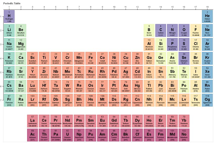
mendeleev Documentation, Release 0.9.0

 (continued from previous page)
 spin='HS',
 ),
 IonicRadius(
 atomic_number=26,
 charge=2,
 coordination='VIII',
 crystal_radius=106.0,
 econf='3d6',
 id=153,
 ionic_radius=92.0,
 most_reliable=False,
 origin='calculated, ',
 spin='HS',
 )]

 Appropriate value of ionization energy and electron affinity are available under ie and ea attributes

 [9]: fe_2.ie
 [9]: 30.651

[10]: fe_2.ea
[10]: 16.1992

 compute ionic potential

[11]: fe_2.ionic_potential()
[11]: 0.02564102564102564

 3.5 Visualizing custom periodic tables

 In this tutorial you’ll how to use mendeleev to create customized visualizations of the periodic table.
 The most convenient method to use for this is periodic_table function from mendeleev.vis module.

 [1]: from mendeleev.vis import periodic_table

 Make sure you you have optional vis dependencies installed when installing mendeleev. If you are using pip install
 with

 pip install mendeleev[vis]

 To see the default visualization of the periodic table simply call the imported function

 [2]: periodic_table()

 Data type cannot be displayed: application/vnd.plotly.v1+json, text/html

 3.5. Visualizing custom periodic tables 25
mendeleev Documentation, Release 0.9.0

 mendeleev stores also two color schemes for atoms that are frequently used for visualizing molecular structures. One
 set is stored in the cpk_color column and refers to CPK coloring, another is stored in jmol_color column and is used
 by the Jmol program, finally there is also coloring scheme from MOLCAS GV program store in the molcas_gv_color
 attribute. They can be displayed either by hovering of the element to display a tooltip or used directly to color the
 element cells.

[3]: periodic_table(colorby='jmol_color', title="JMol Colors")

 Data type cannot be displayed: application/vnd.plotly.v1+json, text/html

[4]: periodic_table(colorby='cpk_color', title='CPK Colors')

 Data type cannot be displayed: application/vnd.plotly.v1+json, text/html

[5]: periodic_table(colorby='molcas_gv_color', title='MOLCAS GV Colors')

 Data type cannot be displayed: application/vnd.plotly.v1+json, text/html

 3.5.1 Visualizing properties

 Any of the properties in mendeleev can now be visualized and color coded. This means that the value of selected
 attribute will be visible on each element and also it is possible to use the attribute to color code the background of each
 element.
 Let’s first use the covalent_radius_pyykko and display the values with the default color coding by series

[6]: periodic_table(attribute='covalent_radius_pyykko', title="Covalent Radii of Pyykko")

 Data type cannot be displayed: application/vnd.plotly.v1+json, text/html

 Now let’s use the same attribute but in addition color code by the actual values, by adding colorby='attribute'
 argument

[7]: periodic_table(attribute='covalent_radius_pyykko', colorby='attribute',␣
 ˓→title="Covalent Radii of Pyykko")

 Data type cannot be displayed: application/vnd.plotly.v1+json, text/html

 The color map can aslo be csutomized using the cmap argument to any of the standard colormaps available in matplotlib

[8]: periodic_table(attribute='covalent_radius_pyykko', colorby='attribute',
 cmap='spring', title="Covalent Radii of Pyykko")

 Data type cannot be displayed: application/vnd.plotly.v1+json, text/html

 26 Chapter 3. Tutorials
mendeleev Documentation, Release 0.9.0

 Let also see one of the more modern colormaps: viridis, plasma, inferno and magma.

 [9]: periodic_table(attribute='covalent_radius_pyykko', colorby='attribute',
 cmap='inferno', title="Covalent Radii of Pyykko")

 Data type cannot be displayed: application/vnd.plotly.v1+json, text/html

 Lets try a different property: atomic_volume

[10]: periodic_table(attribute='atomic_volume', colorby='attribute', title='Atomic Volume')

 Data type cannot be displayed: application/vnd.plotly.v1+json, text/html

[11]: periodic_table(attribute='en_pauling', colorby='attribute',
 title="Pauling's Electronegativity", cmap='viridis')

 Data type cannot be displayed: application/vnd.plotly.v1+json, text/html

 3.5.2 Wide 32-column version

 The periodic_table function can also present the periodic table in the so-called wide format with the f -block between
 the s- and d-blocks resulting in 32 columns.

[12]: periodic_table(height=600, width=1500, wide_layout=True)

 Data type cannot be displayed: application/vnd.plotly.v1+json, text/html

 3.6 Advanced visulization tutorial

 mendeleev support two interactive plotting backends
 1. Plotly (default)
 2. Bokeh

 3.6.1 Note

 Depending on your environment being the classic jupyter notebook or jupyterlab you might have to do additional
 configuration steps, so if you’re not getting expected results see plotly of bokeh documentation.

 3.6. Advanced visulization tutorial 27
mendeleev Documentation, Release 0.9.0

 3.6.2 Accessing lower level plotting functions

 There are two plotting functions for each of the backends:
 • periodic_table_plotly in mendeleev.vis.plotly
 • periodic_table_bokeh in mendeleev.vis.bokeh
 that you can use to customize the visualizations even further.
 Both functions take the same keyword arguments as the periodic_table function but the also require a DataFrame
 with periodic table data. You can get the default data using the create_vis_dataframe function. Let’s start with an
 example using the plotly backend.

[1]: from mendeleev.vis import create_vis_dataframe, periodic_table_plotly

[2]: elements = create_vis_dataframe()
 periodic_table_plotly(elements)

 Data type cannot be displayed: application/vnd.plotly.v1+json, text/html

 3.6.3 Custom coloring scheme

 You can also add a custom color map by assigning color to all the elments. This can be done by creating a custom
 column in the DataFrame and then using colorby argument to specify which column contains colors. Let’s try to
 color the elements according to the block they belong to.

[3]: import seaborn as sns
 from matplotlib import colors
 blockcmap = {b : colors.rgb2hex(c) for b, c in zip(['s', 'p', 'd', 'f'], sns.color_
 ˓→palette('deep'))}

 elements['block_color'] = elements['block'].map(blockcmap)
 periodic_table_plotly(elements, colorby='block_color')

 Data type cannot be displayed: application/vnd.plotly.v1+json, text/html

 3.6.4 Custom properties

 You can also create your own properties to be displayed using pandas awesome methods for manipulating data. For
 example let’s consider the difference of electronegativity between every element and the Oxygen atom. To calculate
 the values we will use Allen scale this time and call our new value ENX-ENO.

[4]: elements.loc[:, 'ENX-ENO'] = elements.loc[elements['symbol'] == 'O', 'en_allen'].values␣
 ˓→- elements.loc[:, 'en_allen']

 periodic_table_plotly(elements, attribute='ENX-ENO', colorby='attribute',
 cmap='viridis', title='Allen Electronegativity wrt. Oxygen')

 28 Chapter 3. Tutorials
mendeleev Documentation, Release 0.9.0 (continued from previous page) Data type cannot be displayed: application/vnd.plotly.v1+json, text/html As a second example let’s consider a difference between the covalent_radius_slater and covalent_radius_pyykko values [5]: elements['cov_rad_diff'] = elements['atomic_radius'] - elements['covalent_radius_pyykko'] periodic_table_plotly(elements, attribute='cov_rad_diff', colorby='attribute', title='Covalent Radii Difference', cmap='viridis') Data type cannot be displayed: application/vnd.plotly.v1+json, text/html 3.6.5 Bokeh backend We can also use the Bokeh backed in the same way but we need to take a few extra steps to render the result in a notebook [6]: from bokeh.plotting import show, output_notebook from mendeleev.vis import periodic_table_bokeh First we need to enable notebook output [7]: output_notebook() Data type cannot be displayed: application/javascript, application/vnd.bokehjs_load.v0+json [8]: fig = periodic_table_bokeh(elements) show(fig) Data type cannot be displayed: application/javascript, application/vnd.bokehjs_exec.v0+json [9]: fig = periodic_table_bokeh(elements, attribute="atomic_radius", colorby="attribute") show(fig) Data type cannot be displayed: application/javascript, application/vnd.bokehjs_exec.v0+json 3.6. Advanced visulization tutorial 29
mendeleev Documentation, Release 0.9.0

3.7 Jupyter notebooks

All tutorials are available as Jupyter notebooks on binder where you can explore the examples interactively:
 • Quick start
 • Bulk data access
 • Electronic Configuration
 • Ions
 • Visualizations
 • Advanced visualizations

30 Chapter 3. Tutorials
CHAPTER

 FOUR

 DATA

To find out how to fetch data in bulk, check out the documentation about data access.

4.1 Elements

The followig data are currently available:

 Name Type Comment Unit Data Source
 abundance_crust float Abundance in the mg/kg [22]
 Earth’s crust
 abundance_sea float Abundance in the mg/L [22]
 seas
 annotation str Annotations regard-
 ing the data
 atomic_number int Atomic number
 atomic_radius float Atomic radius pm [49]
 atomic_radius_rahm float Atomic radius by pm [41, 42]
 Rahm et al.
 atomic_volume float Atomic volume cm3 /mol
 atomic_weight float Atomic weight1 [32, 60]
 atomic_weight_uncertainty
 float Atomic weight un- [32, 60]
 certainty?
 block str Block in periodic ta-
 ble
 boiling_point float Boiling temperature K
 c6 float C_6 dispersion co- a.u. [13, 52]
 efficient in a.u.
 c6_gb float C_6 dispersion a.u. [21]
 coefficient in a.u.
 (Gould & Bučko)
 cas str Chemical Abstracts
 Serice identifier
 cova- float Covalent radius by pm [10]
 lent_radius_bragg Bragg
 cova- float Covalent radius by pm [16]
 lent_radius_cordero Cerdero et al.2
 continues on next page

 31
mendeleev Documentation, Release 0.9.0

 Table 1 – continued from previous page
 Name Type Comment Unit Data Source
 cova- float Single bond co- pm [39]
 lent_radius_pyykko valent radius by
 Pyykko et al.
 cova- float Double bond co- pm [38]
 lent_radius_pyykko_double valent radius by
 Pyykko et al.
 cova- float Triple bond covalent pm [40]
 lent_radius_pyykko_triple radius by Pyykko et
 al.
 cpk_color str Element color in HEX [57]
 CPK convention
 density float Density at 295K10 g/cm3 [22, 63]
 description str Short description of
 the element
 dipole_polarizability float Dipole polarizabil- a.u. [47]
 ity
 dipole_polarizability_unc
 float Dipole polarizabil- a.u. [47]
 ity uncertainty
 discoverers str The discoverers of
 the element
 discovery_location str The location where
 the element was dis-
 covered
 dipole_year int The year the element
 was discovered
 electron_affinity float Electron affinity3 eV [6, 22]
 electrons int Number of electrons
 electrophilicity float Electrophilicity eV [35]
 index
 en_allen float Allen’s scale of elec- eV [28, 29]
 tronegativity4
 en_ghosh float Ghosh’s scale of [18]
 electronegativity
 en_mulliken float Mulliken’s scale of eV [33]
 electronegativity
 en_pauling float Pauling’s scale of [22]
 electronegativity
 econf str Ground state elec-
 tron configuration
 evaporation_heat float Evaporation heat kJ/mol
 fusion_heat float Fusion heat kJ/mol
 gas_basicity float Gas basicity kJ/mol [22]
 geochemical_class str Geochemical classi- [55]
 fication
 glawe_number int Glawe’s number [19]
 (scale)
 goldschmidt_class str Goldschmidt classi- [55, 56]
 fication
 group int Group in periodic
 table
 continues on next page

32 Chapter 4. Data
mendeleev Documentation, Release 0.9.0

 Table 1 – continued from previous page
 Name Type Comment Unit Data Source
 heat_of_formation float Heat of formation kJ/mol [22]
 ionenergy tuple Ionization energies eV [23]
 ionic_radii list Ionic and crystal pm [26, 48]
 radii in pm9
 is_monoisotopic bool Is the element
 monoisotopic
 is_radioactive bool Is the element ra-
 dioactive
 isotopes list Isotopes
 jmol_color str Element color in HEX [61]
 Jmol convention
 lattice_constant float Lattice constant Angstrom
 lattice_structure str Lattice structure
 code
 mass_number int Mass number (most
 abundant isotope)
 melting_point float Melting temperature K
 mendeleev_number int Mendeleev’s num- [37, 53]
 ber5
 metallic_radius float Single-bond metal- pm [1]
 lic radius
 metallic_radius_c12 float Metallic radius with pm [1]
 12 nearest neighbors
 molcas_gv_color str Element color HEX [62]
 in MOCAS GV
 convention
 name str Name in English
 name_origin str Origin of the name
 neutrons int Number of neutrons
 (most abundant iso-
 tope)
 oxistates list Oxidation states
 period int Period in periodic
 table
 pettifor_number float Pettifor scale [37]
 proton_affinity float Proton affinity kJ/mol [22]
 protons int Number of protons
 sconst float Nuclear charge [14, 15]
 screening con-
 stants6
 series int Index to chemical
 series
 sources str Sources of the ele-
 ment
 specific_heat float Specific heat @ 20 C J/(g mol)
 symbol str Chemical symbol
 ther- float Thermal conductiv- W/(m K)
 mal_conductivity ity @25 C
 uses str Applications of the
 element
 continues on next page

4.1. Elements 33
mendeleev Documentation, Release 0.9.0

 Table 1 – continued from previous page
 Name Type Comment Unit Data Source
 vdw_radius float Van der Waals ra- pm [22]
 dius
 vdw_radius_alvarez float Van der Waals pm [5, 54]
 radius according to
 Alvarez7
 vdw_radius_batsanov float Van der Waals pm [8]
 radius according to
 Batsanov
 vdw_radius_bondi float Van der Waals pm [9]
 radius according to
 Bondi
 vdw_radius_dreiding float Van der Waals ra- pm [31]
 dius from the DREI-
 DING FF
 vdw_radius_mm3 float Van der Waals ra- pm [3]
 dius from the MM3
 FF
 vdw_radius_rt float Van der Waals pm [44]
 radius according to
 Rowland and Taylor
 vdw_radius_truhlar float Van der Waals pm [30]
 radius according to
 Truhlar
 vdw_radius_uff float Van der Waals ra- pm [43]
 dius from the UFF

 1 Atomic Weights

 Atomic weights and their uncertainties were retrieved mainly from ref. [60]. For elements whose values were given as ranges the conventional
atomic weights from Table 3 in ref. [32] were taken. For radioactive elements the standard approach was adopted where the weight is taken as
the mass number of the most stable isotope. The data was obtained from CIAAW page on radioactive elements. In cases where two isotopes were
specified the one with the smaller standard deviation was chosen. In case of Tc and Pm relative weights of their isotopes were used, for Tc isotope
98, and for Pm isotope 145 were taken from CIAAW.
 2 Covalent Radius by Cordero et al.

 In order to have a more homogeneous data for covalent radii taken from ref. [16] the values for 3 different valences for C, also the low and high
spin values for Mn, Fe Co, were respectively averaged.
 10 Densities

 Density values for solids and liquids are always in units of grams per cubic centimeter and can be assumed to refer to temperatures near room
temperature unless otherwise stated. Values for gases are the calculated ideal gas densities at 25°C and 101.325 kPa.
 Original values for gasses are converted from g/L to g/cm3 .
 For elements where several allotropes exist, the density corresponding to the most abundand are reported (for full list refer to [22]), namely:
 • Antimony (gray)
 • Berkelium ( form)
 • Carbon (graphite)
 • Phosphorus (white)
 • Selenium (gray)
 • Sulfur (rhombic)
 • Tin (white)
 For elements where experimental data is not available, theoretical estimates taken from [63] are used, namely for:
 • Astatine
 • Francium
 • Einsteinium
 • Fermium
 • Mendelevium

34 Chapter 4. Data
mendeleev Documentation, Release 0.9.0

4.2 Isotopes

 Name Type Comment Unit Data Source
 abundance float Relative Abundance [59]
 g_factor float Nuclear g-factor8 [51]
 half_life float Half life of the iso- [32]
 tope
 half_life_unit str Unit in which the [32]
 half life is given
 is_radioactive bool Is the isotope ra- [58]
 dioactive
 mass float Atomic mass Da [58]
 mass_number int Mass number of the [58]
 isotope
 mass_uncertainty float Uncertainty of the [58]
 atomic mass
 spin float Nuclear spin quan-
 tum number
 quadrupole_moment float Nuclear electric b [100 fm2 ] [50]
 quadrupole mo-
 ment?

 • Nobelium
 • Lawrencium
 • Rutherfordium
 • Dubnium
 • Seaborgium
 • Bohrium
 • Hassium
 • Meitnerium
 • Darmstadtium
 • Roentgenium
 • Copernicium
 • Nihonium
 • Flerovium
 • Moscovium
 • Livermorium
 • Tennessine
 • Oganesson

 3 Electron affinity

 Electron affinities were taken from [22] for the elements for which the data was available. For He, Be, N, Ar and Xe affinities were taken from [6]
where they were specified for metastable ions and therefore the values are negative.
 Updates
 • Electron affinity of niobium was taken from [27].
 • Electron affinity of cobalt was taken from [11].
 • Electron affinity of lead was taken from [12].

 4 Allen’s configuration energies

 The values of configurational energies from refs. [28] and [29] were taken as reported in eV without converting to Pauling units.
 9 Ionic radii for Actinoid (III) ions

 Ionic radii values for 3+ Actinoids were with coordination number 9 were taken from [26]. In addition crystal_radius values were computed
by adding 14 pm to the ionic_radius values according to [48].
 5 Mendeleev numbers

 Mendeleev numbers were mostly taken from [53] but the range was extended to cover the whole periodic table following the prescription in the
article of increasing the numbers going from top to bottom in each group and group by group from left to right in the periodic table.
 6 Nuclear charge screening constants

 The screening constants were calculated according to the following formula
 , , = − · , ,
4.2. Isotopes 35
where is the principal quantum number, is the atomic number, , , is the screening constant, , , is the optimized exponent from [14,
15].
 For elements Nb, Mo, Ru, Rh, Pd and Ag the exponent values corresponding to the ground state electronic configuration were taken (entries with
superscript a in Table II in [15]).
mendeleev Documentation, Release 0.9.0

Data Footnotes

 • In quadrupole moment data - a typo for Ac-227: sign should be +

36 Chapter 4. Data
CHAPTER

 FIVE

 ELECTRONEGATIVITIES

Since electronegativity is useful concept rather than a physical observable, several scales of electronegativity exist and
some of them are available in mendeleev. Depending on the definition of a particular scale the values are either stored
directly or recomputed on demand with appropriate formulas. The following scales are stored:
 • Allen
 • Ghosh
 • Pauling
Moreover there are electronegativity scales that can be computed from their respective definition and the atomic prop-
erties available in mendeleev:
 • Allred-Rochow
 • Cottrell-Sutton
 • Gordy
 • Li and Xue
 • Martynov and Batsanov
 • Mulliken
 • Nagle
 • Sanderson
For a short overview on electronegativity see this presentation.
All the examples shown below are for Silicon:

>>> from mendeleev import element
>>> Si = element('Si')

5.1 Allen

The electronegativity scale proposed by Allen in ref [2] is defined as:
 ∑︀

 = ∑︀

where: is the multiplet-averaged one-electron energy of the subshell and is the number of electrons in subshell
 and the summation runs over the valence shell.
The values that are tabulated were obtained from refs. [28] and [29].

 37
mendeleev Documentation, Release 0.9.0
Example:
>>> Si.en_allen
11.33
>>> Si.electronegativity('allen')
11.33
5.2 Allred and Rochow
The scale of Allred and Rochow [4] introduces the electronegativity as the electrostatic force exerted on the electron
by the nuclear charge:
2 eff
=
2
where: eff is the effective nuclear charge and is the covalent radius.
Example:
>>> Si.electronegativity('allred-rochow')
0.00028240190249702736
5.3 Cottrell and Sutton
The scale proposed by Cottrell and Sutton [17] is derived from the equation:
√︂
eff
=
where: eff is the effective nuclear charge and is the covalent radius.
Example:
>>> Si.electronegativity('cottrell-sutton')
0.18099342720014772
5.4 Ghosh
Ghosh [18] presented a scale of electronegativity based on the absolute radii of atoms computed as
= · (1/ ) +
where: is the absolute atomic radius and and are empirical parameters.
Example:
>>> Si.en_ghosh
0.178503
38 Chapter 5. ElectronegativitiesYou can also read