Numerical simulation of wind loads on an offshore PV panel: the effect of wave angle
←
→
Page content transcription
If your browser does not render page correctly, please read the page content below
Journal of Mechanics, 2020, 37, 53–62
DOI: 10.1093/jom/ufaa010
Regular article

Numerical simulation of wind loads on an offshore PV panel:
                  the effect of wave angle
                               Kao-Chun Su1 , Ping-Han Chung                                   1,∗
                                                                                                     and Ray-Yeng Yang                      2

                                                                                                                                                                                 Downloaded from https://academic.oup.com/jom/article/doi/10.1093/jom/ufaa010/6015294 by guest on 20 December 2020
                      1
                        Department of Aeronautics and Astronautics, National Cheng Kung University, Tainan, Taiwan, Republic of China
                 2
                     Department of Hydraulic and Ocean Engineering, National Cheng Kung University, Tainan, Taiwan, Republic of China
                                                          ∗ Corresponding author: P46084493@mail.ncku.edu.tw

                                                                             A B ST R A C T
This numerical simulation determines the wind loads on a stand-alone solar panel in a marine environment. The initial angle of tilt is 20° and
40° and the wind is incident at an angle of 0–180° (in increments of 45°). The wave angle affects the motion of a pontoon. For a wave angle of
0–180° (in increments of 45°), the variation in the surface pressure pattern and the lift coefficient with the angle of incidence of wind and waves
in a single period is determined. The lift force is determined by competing the tilt angle for the upper surface with respect to wind and variation
in roll angle for a specific wave angle. The data are pertinent to structural design for photovoltaic systems in a marine environment.

KEY WOR DS: PV, tilt angle, wind incidence angle, wave angle

                         1. IN TRODUCTION                                                 the spacing, degree of sheltering for the arrays and the clearance
The consumption of fossil fuels and excessive CO2 emis-                                   between the PV array and building roof [19–21].
sions contribute to environmental problems (extreme climate,                                Previous studies were conducted only for wind loads on
air/water pollution) and affect global supply chains [1–3]. The                           rooftop or grounded PV systems. There is greater lift coefficient
use of solar energy has increased and the total capacity for so-                          for a stand-alone panel than for a stand-alone array. Wind loads
lar photovoltaic (PV) systems was 402 GW in 2017 and 640                                  are also significantly reduced by the presence of neighboring up-
GW in 2018 [4]. Renewable energy using PV systems is now a                                wind arrays due to sheltering effect [16, 22]. For a floating PV
mainstream form of electricity generation. In the domestic and                            system in offshore areas, it is subject to the dynamics of tides,
commercial sectors, tilting PV panels are usually mounted on                              wind and waves. Variation in the wave angle, γ , affects the mo-
rooftops to harness solar energy, in which tilt angle of installed                        tion of the pontoon. During a wave cycle T*, wind loads on PV
PV panels has a great influence on the power generation. The                              panels are not the same as those for rooftop or ground-mounted
maximum yearly system performance in the Northern Hemi-                                   PV panels. This study determines the motion of a pontoon using
sphere can be obtained when PV panels are facing south with                               meteorological data from offshore buoys. A schematic drawing
a tilt angle equal to the latitude [5]. Duffie et al. [6] suggested                       for a tilting panel on a pontoon is shown in Fig. 1. The initial an-
the yearly optimal tilt angle of PV panels as latitude ± 15°. For                         gle between the tilting panel and the pontoon, α, is 20° and 40°.
ground-mounted PV systems, land occupancy is a crucial prob-                              A numerical simulation determines the effect of β (= 0–180° in
lem. Floating PV systems in reservoirs, ponds or lakes have be-                           increments of 45°) and γ (= 0–180° in increments of 45°) on
come more common [7, 8]. The offshore PV system floats on a                               wind loads on a stand-alone tilting panel, which is critical for a
pontoon [9].                                                                              system in a harsh marine environment. β and γ are defined as the
   Typhoons or hurricanes are natural hazards that have a costly                          angles between the longitudinal direction (x-axis) of the tilting
effect on residential constructions and their accessories [10].                           panel and wind or waves. The bottom of the tilting panel above
The wind loads on a PV system with tilting panels depend on the                           a pontoon is denoted as h.
tilt angle and the angle of incidence of the wind, β. The greater
the tilt angle, the smaller the value of the lift coefficient, CL , for
a stand-alone panel [11–16], because pressure is equalized at                                               2. NU M ER IC A L M ETHOD
large angles of tilt and turbulence is equalized at small angles                                               2.1 Numerical simulation
of tilt [17]. Chou et al. [18] determined the effect of β. There                          Computational fluid dynamics simulation is used to determine
is greater suction on the upper surface near the windward cor-                            surface pressure patterns and the lift coefficient for a stand-
ner for β = 15–60°. An unsymmetrical pressure pattern due to                              alone tilting panel (full scale, length l = 1640 mm; width
windward vortex results in greater bending moment. The aero-                              w = 992 mm; thickness = 4 mm) and h is 450 mm
dynamic characteristics also depend on the scale of the panels,                           (pontoon: length L = 2000 mm; width W = 2000 mm; height
Received: 13 May 2020; Accepted: 21 September 2020
© The Author(s) 2020. Published by Oxford University Press on behalf of Society of Theoretical and Applied Mechanics of the Republic of China, Taiwan. This is an Open Access
article distributed under the terms of the Creative Commons Attribution License (http://creativecommons.org/licenses/by/4.0/), which permits unrestricted reuse, distribution,
and reproduction in any medium, provided the original work is properly cited.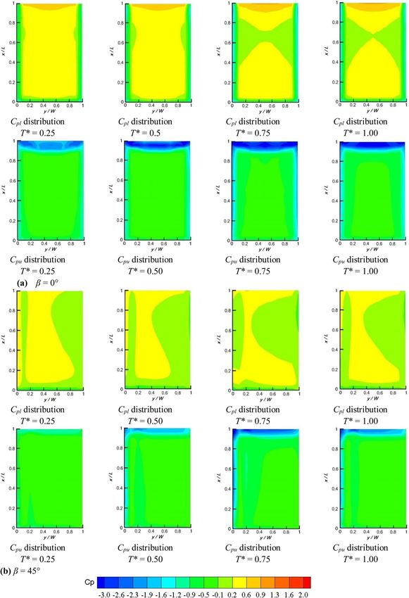
54 • Journal of Mechanics, 2020, Vol. 37
strong adverse pressure gradients, separation and recirculation
[24].
∂ (ρk) ∂ ρku j ∂ uf ∂k
+ = u+
∂t ∂x j ∂x j σk ∂x j
+ Gk + Gb − ρε − YM − Sk , (3)
∂ (ρε) ∂ ρεu j ∂ ut ∂ε
+ = u+
∂t ∂x j ∂x j σε ∂x j
Downloaded from https://academic.oup.com/jom/article/doi/10.1093/jom/ufaa010/6015294 by guest on 20 December 2020
ε2 ε
+ ρC1 Sε − ρC2 √ + C1ε C3ε Gb − Sε , (4)
k + vε k
where
η
C1 = max 0.43 , (5)
η+5
k
η = S , (6)
ε
S = 2Sij Sij , (7)
where Gk and Gb represent the generation of turbulence ki-
netic energy due to mean velocity gradients and buoyancy, re-
spectively. YM is the contribution of the fluctuation dilatation
in compressible turbulence to the overall dissipation rate. σ k
and σ ε are the turbulent Prandtl numbers for k and ε, while
C2 and C1ε are constants. Sk and Sε are user-defined source
terms.
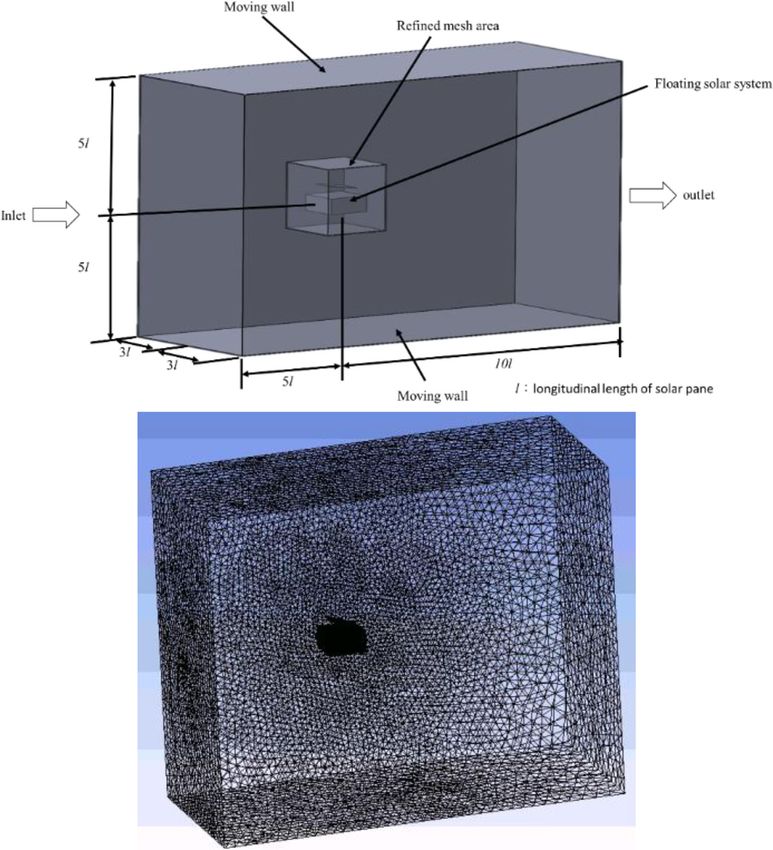
The computational domain and grid are created using the grid
generation software, Pointwise, as shown in Fig. 2. The tilted
panel is placed in a computational domain with spatial dimen-
sion of 15L (length) × 6L (width) × 10L (height), with an
upstream fetch of 5L and a downstream length of 10L. The ve-
Figure 1 A schematic drawing of a tilting panel on a pontoon.
locity at the inlet (uniform flow) is 20 m/s and the turbulence
H = 500 mm). 3D Reynolds-averaged Navier–Stokes simu- intensity is 0.3%. There are stationary, no slip, non-penetrating
lations (commercial ANSYS Fluent software, version 13) use and adiabatic side walls. Moving upper and lower walls, corre-
a steady finite volume solver of second-order accuracy with a sponding to variation in the tilt angle of solar panel, are used. The
steady inlet. A semi-implicit method for pressure-linked equa- numerical meshes are determined using a grid sensitivity study
tion is used. The conservation equations are solved: for grids of 35–50 million cells. The variation in the value of
Cp (= (p − p∞ )/q) for α = 20° and γ = β = 0° is 0.14% for 35
∂ρ and 50 million grids, where p∞ is the freestream static pressure
+∇ · (ρṽ) = 0, (1)
∂t and q is the dynamic pressure. Since there are no experimental
data available for a tilting panel in wave motion, this numerical
simulation is validated for a ground-mounted tilting panel (α =
∂V
ρ + V · ∇V = −∇ p + μ∇ 2V + f, (2) 20° and β = 0°) [25]. Figure 3 shows that the agreement for lon-
∂t
gitudinal pressure distribution on the upper and lower surfaces
where ρ, v, p, μ and f are, respectively, the air density, the velocity is reasonably well.
component, the dynamic viscosity and the body force.
Although an SST κ–ω turbulence model [23] is used for many 2.2 Motion of a pontoon
aerodynamic applications, it requires meshing down (or more Waves are non-stationary in nature. Meteorological data were
computational time). For a tilt panel, the flow is dominated by collected from offshore buoys in Taiwan (Qigu, Longdong and
leading-edge separation, side-edge vortices and windward vor- Hsinchu). The historical records (2013–17) show that common
tex. A realizable κ–ε turbulence model with a first grid point of values of β and γ vary significantly between buoys [26]. The
y+ ∼ 30 is used for this parametric analysis. The model exhibits maximum wave height was 17.12 m and the period T was 15.1
superior performance for flows involving boundary layers under s during Typhoon Soudelor in 2015, in which a stationary sine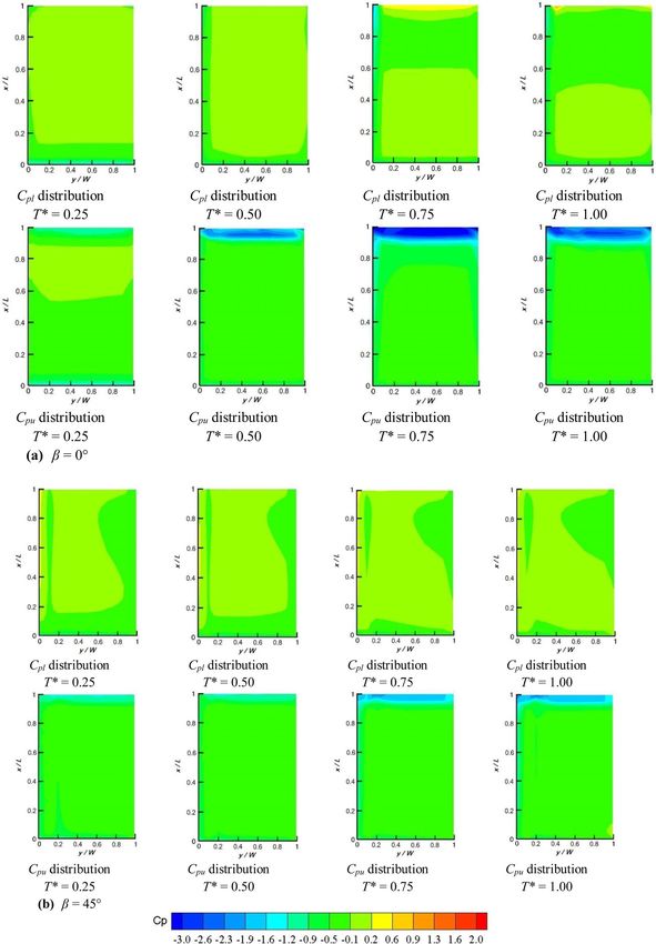
Numerical simulation of wind loads on an offshore PV panel   • 55

                                                                                                                                                 Downloaded from https://academic.oup.com/jom/article/doi/10.1093/jom/ufaa010/6015294 by guest on 20 December 2020
Figure 2 Computational domain and mesh.

                                                                          wave is used for this simulation. The motion of a pontoon is
                                                                          simulated using ANSYS AQWA software, which is used exten-
                                                                          sively for assessment of all types of offshore and marine struc-
                                                                          tures [27]. Since air flow is influenced by the wave surface, the
                                                                          deviation in the tilt angle on the upper surface from α, α u ,
                                                                          and the variation in the roll angle with respect to the x-direction,
                                                                          Rx , are determined for β = 0–180° (in increments of 45°) and
                                                                          γ = 0–180° (in increments of 45°). The values of α u during
                                                                          a wave cycle are shown in Fig. 4. The value of α u for γ = 0°
                                                                          and 45° is initially negative and then positive. The peak values
                                                                          are −12.5° (0.22T) and 9.9° (0.72T) for γ = 0°. For α = 20°,
                                                                          the tilt angle for the upper surface with respect to wind direc-
                                                                          tion, α u , is 7.5−29.9°. Su et al. [28] showed that there is an in-
                                                                          crease in the wind loads as the initial angle of tilt increases and
                                                                          lift force is less at low angles of incidence for the wind. For γ =
                                                                          45°, the value of α u ranges from −7.9° (0.25T) to 8.1° (0.72T).
Figure 3 Longitudinal surface pressure distribution for a tilting panel   The variation in Rx (= −11.4° to 12.3°) is similar to that for
for α = 20° and β = 0°.                                                      α u . For γ = 90°, the value of α u is fixed and the value of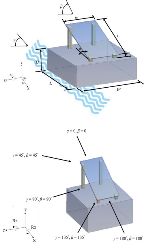
56   • Journal of Mechanics, 2020, Vol. 37

Figure 4 Motion of a pontoon.                                                                                                           Downloaded from https://academic.oup.com/jom/article/doi/10.1093/jom/ufaa010/6015294 by guest on 20 December 2020

Rx (= −15.9° to 16.4°) is greater. The opposite trend for                    3. R ESULTS A ND DISCUSSION
   α u and Rx is true for γ = 135°, i.e. α u = −16.0° to                          3.1 Surface pressure patterns
16.4° and Rx = −8.8° to 8.9°. If the lower surface faces the
                                                                  The distributions of surface pressure (α = 20° and γ = 45°)
wave (γ = 180°), the value of Rx is fixed. The value of
                                                                  on the upper Cpu and lower Cpl surfaces for T* = 0.25, 0.5,
   α u is initially positive and then negative. The peak values
                                                                  0.75 and 1.00 are shown in Fig. 5. For β = 0° (Fig. 5a), there
are 18.7° (0.22 T) and −15.8° (0.77 T), so variation in γ
                                                                  is a symmetrical surface pattern with respect to the middle line
has a significant effect on the value of α u . Since the yearly
                                                                  (y/w = 0.5) during a wave cycle. At T* = 0.25, α u has a neg-
optimal tilt angle of PV panels corresponds to the local lat-
                                                                  ative value (= −7.9°), so there is a decrease in the velocity nor-
itude ± 15° [6], the effect of γ on the maximum yearly
                                                                  mal to the lower surface. Chou et al. [16] showed that the up-
system performance may be neglected in this simulated sea
                                                                  ward force for a tilted panel increases linearly with increasing α.
environment.
Numerical simulation of wind loads on an offshore PV panel • 57
Downloaded from https://academic.oup.com/jom/article/doi/10.1093/jom/ufaa010/6015294 by guest on 20 December 2020
Figure 5 Surface pressure distributions for α = 20° and γ = 45°: (a) β = 0° and (b) β = 45°.
However, the values of Cpl for x/L = 0.35–0.85 at T* = 0.25 edge due to flow separation, following an increase when flow
(Rx = −11.2°) are greater than those at T* = 0.75 ( α u = 7.6°, is reattached. Side-edge vortices form, so the value of Cpu de-
Rx = 11.4°) and T* = 1.00 ( α u = 0.1°). This demonstrates creases. Figure 5b shows the distributions of Cpu and Cpl for
the effect of Rx ; i.e. if Rx has a negative value, the value of Cpl β = 45°. The surface pressure patterns on the upper and lower
increases. On the upper surface, there is suction near the front surfaces are not symmetrical. The value of Cpl near the front edge58 • Journal of Mechanics, 2020, Vol. 37
Downloaded from https://academic.oup.com/jom/article/doi/10.1093/jom/ufaa010/6015294 by guest on 20 December 2020
Figure 6 Surface pressure distributions for α = 20° and γ = 135°: (a) β = 0° and (b) β = 45°.
is less than that for β = 0° and the effect of β is more signif- For γ = 135° and α = 20°, the value of α u ranges from
icant at T* = 0.75 and T* = 1.00. A windward corner vortex −16.0° (T* = 0.22) to 16.4 (T* = 0.72). The lower surface
(suction near x/L = 1 and y/W = 0) forms on the upper surface, is ∼4° to the wind direction at T* = 0.22. The variation in Rx
particularly at T* = 0.75, which corresponds to a greater value shows an opposite trend. The distributions for Cpu and Cpl for
for α u . β = 0° are shown in Fig. 6a. On the lower surface, the valueNumerical simulation of wind loads on an offshore PV panel • 59
Downloaded from https://academic.oup.com/jom/article/doi/10.1093/jom/ufaa010/6015294 by guest on 20 December 2020
Figure 7 Lift coefficient, α = 20°: (a) γ = 45°, (b) γ = 90°, (c) γ = 135°, and (d) γ = 180°.
of Cpl is lower than that for γ = 45°. The surface pressure pat- β for a wave cycle for α = 20°. For γ = 0°, Su et al. [28] deter-
tern is slightly unsymmetrical, particularly at T* = 0.75. There mined that there is an increase in wind loads at low β. Figure 7a
is greater suction at the left corner near the front edge. The value shows that for γ = 45°. The value of CL is negative for β = 0°
of Rx is −8.7° for greater values of Cpl near the front edge. On the and 45° and positive for β = 135° and 180°. The value of CL is
upper surface, the value of α u ranges from 4.0° to 36.4° during lower for β = 0°. This is not consistent with the results of a previ-
a wave cycle. There is greater suction near the front edge due to ous study by Chou et al. [18], which determined that the lowest
flow separation at T* = 0.72. This result is in agreement with that CL value for a ground-mounted tilted PV panel at a specific value
of a previous study by Stathopoulos et al. [13], which demon- of α is observed for β = 30°. The lift force on a tilted PV panel
strated that an increase in α results in greater suction. in a marine environment depends on a combination of β and γ
The distributions for Cpu and Cpl for β = 45° are shown in (or Rx ) effects. For β = 45–135°, there is variation in CL , i.e. an
Fig. 6b. On the lower surface, the surface pressure pattern is not increment during the first quarter of the wave cycle followed by
symmetrical, particularly in the first half region. This is due to a decrease for T* = 0.25–0.75. This is opposite to the variation
the combined effect of windward vortex and side-edge cortices. in α u and Rx for a wave cycle, as shown in Fig. 4. For β = 180°,
In the spanwise direction, there is a lower pressure region close there is a gradual increase until T* = 0.75. For γ = 90°, Fig. 7b
to y/w = 0.1. An increase in α u results in a greater value for Cpl shows that the value of α u is 0° and the variation in Rx resem-
and variation in Rx has an opposite trend. The combined effect of bles a cosine function. The variation in the value of CL is oppo-
α u and Rx then results in a similar surface pressure pattern for site to that for γ = 45°. For the first half of the wave cycle, the
T* = 0.25 and T* = 0.75, and for T* = 0.50 and T* = 1.00. On value of CL is slightly greater for β = 45° than for β = 0°. This is
the upper surface, there is less suction near the front edge than also true for β = 135° (the greatest value for CL ) and β = 180°.
that for β = 0°, so there is greater lift force for β = 45°. This is not Note that the CL distribution (= 1.252 ± 0.025) for β = 180°
consistent with the results of Chou et al. [18], which show less is flatter over the wave cycle. The variation in α u and Rx for
lift force for β = 15–60°. The variation in γ ( α u and Rx ) is a γ = 135° (Fig. 4) is opposite. The average value of CL for a given
factor in determining the wind loads on a tilted panel in a marine β is slightly less than that for γ = 90° (1.3–1.6%). There is a peak
environment. for CL (= 1.541, Fig. 7c) at T* = 0.75 for β = 180°. The value of
Rx is 0° for γ = 180°. The distribution for CL for β = 0° and 45°
3.2 Lift coefficient is similar to that for γ = 90° (Fig. 7d). If the value of Rx (γ =
CL is calculated by integrating the differential pressure between 90°) is negative, the value of CL is decreased but a positive value
upper and lower surfaces. Figure 7 shows the variation in CL with for α u has a similar effect. The variation in CL for β = 135°60 • Journal of Mechanics, 2020, Vol. 37
Downloaded from https://academic.oup.com/jom/article/doi/10.1093/jom/ufaa010/6015294 by guest on 20 December 2020
Figure 8 Lift coefficient, α = 40°: (a) γ = 45°, (b) γ = 90°, (c) γ = 135°, and (d) γ = 180°.
and 180° shows the effect of α u . It is also noted that the abso- the wave cycle and the CL distribution is similar to that for β
lute value of CL for β = 180° (a flip-over panel) is not exactly the = 0°. For β = 90–180°, the opposite relationship between CL
same as that for β = 0°. This is due to presence of a pontoon (or with α u and Rx means that Rx has a dominant effect during a
ground effect). wave cycle. For γ = 90°, the CL distributions are similar to those
The distribution of CL for α = 40° is shown in Fig. 8. For for α = 20°, but not similar to those for γ = 135°. Figure 8c
β = 0° and 45°, the value of CL for α = 40° is less than that shows that there is a gradual increase in CL and a peak value at
for α = 20°. There is an opposite trend for β = 135° and 180°. T* = 0.75 for β = 0° and 45°. In the first half of the wave cy-
This result is in agreement with that for the study by Chou cle (α u < 40°), CL increases due to the effect of α u and Rx . For
et al. [16]. For a stand-alone tilting panel, CL decreases when T* = 0.5–0.75, α u (= 40–55.5°) has a more dominant effect. For
α (≤40°) increases for β ≤ 75° and the opposite is true for β β = 135° and 180°, there is a maximum value for CL at T* = 0.5
= 90–180°. Figure 8a shows that the respective value of CL for (α u = 45.5° and Rx = −3.8°). There is an increase in the down-
γ = 45° is −1.598 ± 0.148 and −1.190 ± 0.092 for β = 0° ward force from the left to right edges. For γ = 180° (Rx = 0°),
and 45°. For α = 20°, the respective values are −0.957 ± 0.047 Fig. 8d shows that the distribution of CL depends on α u and
and −0.784 ± 0.091. For β = 135° and 180°, the values are α u.
1.298 ± 0.249 and 1.735 ± 0.110 for α = 40°, while the val- The lift force on a tilted PV panel in a marine environment is
ues are 1.167 ± 0.079 and 1.201 ± 0.114 for α = 20°. There is determined by a combination of the effect of β and γ ( α u and
a more significant difference in the value of CL for β = 0° and Rx ). A negative value for Rx or a positive value for α u results
45°, and for β = 135° and 180° for α = 40°. The variation in in a decrease in the value of CL . The variation in α u with Rx is
CL for β = 0° shows an opposite trend to that for α u and Rx shown in Fig. 9. For γ = 45°, there is an increase in the value of
in the first quarter of the wave cycle. The CL has a maximum Rx for the value of α u from −7.9° to 7.6°. An opposite trend is
value at T* = 0.75, which corresponds to the peak α u and Rx . determined for γ = 135°. The variation in CL with α u , Rx and β
A negative value for Rx or a positive value for α u results in a is shown in Figs 10 and 11. Note that the value of Rx is ∼0° for
decrease in the value of CL , so α u has a greater effect at the α u of 20° and 40°. For α = 20°, there is a small difference (1.4%)
beginning of the wave cycle for α u = 32–40°. Chou et al. [16] in the value of CL /Rx for β = 0° and β = 45° due to the op-
determined that the value of CL for α = 40–50° increases as the posing effects of β and Rx . The difference is more significant for
value of α increases. The value of CL is a maximum at T* = 0.75 α = 40°. For γ = 45°, the value of Rx (= −11.2° to −3.9°) is
for α u = 47.6°. The values of α u and Rx have an obvious ef- negative for the value of α u from −7.9° to −3.6°. There is a
fect. For β = 45°, the α u effect is less for the first quarter of significant increase in CL /Rx as α u increases. If the value of Rx isNumerical simulation of wind loads on an offshore PV panel • 61
or α u = 42.9–47.6° for negative Rx . Chou et al. [16] determined
that the value of CL for α = 40–50° increases as α increases, so
the value of α u has a dominant effect on the variation in CL .
4. CONCLUSIONS
For a tilting PV panel mounted on rooftop or ground, the criti-
cal wind loads are observed at lower angles of incidence for the
wind (= 15–60°), when the angle of tilt for the panel is >30°.
This study determines the wind loads on an offshore PV panel
Downloaded from https://academic.oup.com/jom/article/doi/10.1093/jom/ufaa010/6015294 by guest on 20 December 2020
throughout a wave cycle. A change in deviation in tilt angle and
roll angle corresponds to variation in wave angle. On the upper
surface, the surface pressure pattern depends on the flow sepa-
ration near the front edge and the formation of side-edge and
windward vortices. As the deviation in tilt angle increases, the
value of surface pressure on the lower surface increases and the
variation in roll angle has an opposite trend. On the lower sur-
Figure 9 α u versus Rx for γ = 45° and 135°. face, a negative value of roll angle results in an increase in the
value of surface pressure on the lower surface, and the effect of
positive, increasing α u ( α u = 2.9–7.6°) has a less effect. The angle of wind incidence varies during a wave cycle. If the span-
effect of α u and Rx is combined. For γ = 135°, there is an oppo- wise pressure distribution is unsymmetrical, the bending mo-
site trend in the variation in α u and Rx . CL is affected by the ment in increased. The value of lift coefficient is affected by ini-
values of α u and Rx . CL /Rx decreases significantly for α = 40° tial tilt angle, deviation in tilt angle, angle of wind incidence and
Figure 10 Lift coefficient for γ = 45°.
Figure 11 Lift coefficient for γ = 135°.62 • Journal of Mechanics, 2020, Vol. 37
roll angle, i.e. a combination of all of the effects during a wave 8. Kim SM, Oh M, Park HD. Analysis and prioritization of the floating
cycle. However, initial tilt angle and deviation in tilt angle (or photovoltaic system potential for reservoirs in Korea. Applied Sciences
wave angle) are dominant factors for a tilting PV panel floating 2019;9:365.
9. Trapani K, Millar DL, Smith HCM. Novel offshore application of
on a pontoon. In addition, the tilt angle of PV panels is associated photovoltaics in comparison to conventional marine renewable en-
with the local meteorological data. To maximize the yearly PV ergy technologies. Renewable Energy 2013;50:879–888.
panel performance, motion of a pontoon should be taken into 10. Holmes JD. Rational wind-load design and wind-load factors for lo-
account for design of PV systems. cations affected by tropical cyclones, hurricanes, and typhoons. In:
Structure Congress 2010, Orlando, FL, 12–15 May 2010.
11. Hsu CC, Huang CI. Vortex simulations of the flow-field of a flat plate
NOM ENCL ATURE with a non-zero angle of attack. Journal of Mechanics 2008;24:N35–
N38.
CL = lift coefficient 12. Shademan M, Hangan H. Wind loading on solar panels at different
Downloaded from https://academic.oup.com/jom/article/doi/10.1093/jom/ufaa010/6015294 by guest on 20 December 2020
Cp = pressure coefficient, (p − p∞ )/q inclination angles. In: Proceedings of the 11th Americas Conference on
Cpl = pressure coefficient on the lower surface Wind Engineering, San Juan, PR, 22–26 June 2009.
Cpu = pressure coefficient on the upper surface 13. Stathopoulos T, Zisis I, Xypnitou E. Local and overall wind pressure
and force coefficients for solar panels. Journal of Wind Engineering and
l = length of tilted panel Industrial Aerodynamics 2014;125:195–206.
p∞ = freestream static pressure 14. Guo M, Zang H, Gao S, Chen T, Xiao J, Cheng L, Wei Z, Sun G. Op-
q = dynamic pressure timal tilt angle and orientation on photovoltaic modules using HS al-
Rx = variation in the roll angle with respect to the x-direction gorithm in different climates in China. Applied Sciences 2017;7:1028.
T = period 15. Su KC, Chung KM, Hsu ST. Numerical simulation of wind loads on
T* = normalized period solar panels. Modern Physics Letters B 2018;32:1840009.
16. Chou CC, Chung PH, Yang RY. Wind loads on a solar panel at high
w = width of tilted panel tilt angles. Applied Sciences 2019;9:1594.
x = coordinate in the longitudinal direction 17. Cao J, Yoshida A, Saha PK, Tamura Y. Wind loading characteristics
y = coordinate in the spanwise direction of solar arrays mounted on flat roofs. Journal of Wind Engineering and
α = tilt angle between a tilt panel and a pontoon Industrial Aerodynamics 2013;123:214–225.
α u = tilt angle for the upper surface 18. Chou CC, Chung KM, Chang KC. Wind loads of solar water heaters:
wind incidence effect. Journal of Aerodynamics 2014;2014:1–10.
α u = deviation in the tilt angle for the upper surface with re-
19. Aly AM. On the evaluation of wind loads on solar panels: the scale
spect to α issue. Solar Energy 2016;135:423–434.
β = wind incidence angle 20. Warsido WP, Bitsuamlak GT, Barata J, Chowdhury AG. Influence of
γ = wave angle spacing parameters on the wind loading of solar array. Journal of Flu-
ids Structure 2014;48:295–315.
21. Li JY, Tong LW, Wu JM, Pan YM. Numerical investigation of wind
pressure coefficients for photovoltaic arrays mounted on building
R EFER EN CE S roofs. KSCE Journal of Civil Engineering 2019;23:3606–3615.
1. Quadrelli R, Peterson S. The energy–climate challenge: recent 22. Chung PH, Chou CC, Chung CY, Yang RY. Wind loads on a PV ar-
trends in CO2 emissions from fuel combustion. Energy Policy ray. Applied Sciences 2019;9:2466.
2007;35:5938–5952. 23. Menter FR. Two-equation eddy-viscosity turbulence models for en-
2. Mi Z, Guan D, Liu Z, Liu J, Viguié V, Fromer N, Wang Y. Cities: gineering applications. AIAA Journal 1994;32:1598–1605.
the core of climate change mitigation. Journal of Cleaner Production 24. Shih TH, Liou WW, Shabbir A, Yang Z, Zhu J. A new κ–ε eddy-
2019;207:582–589. viscosity model for high Reynolds number turbulent flows: model
3. Ghadge A, Wurtmann H, Seuring S. Managing climate change risks development and validation. Computers & Fluids 1995;24:227–238.
in global supply chains: a review and research agenda. International 25. Chung KM, Chou CC, Chang KC, Chen YJ. Effect of a vertical guide
Journal of Production Research 2019;58:44–54. plate on the wind loading of an inclined flat plate. Wind and Structures
4. REN21. Renewables 2019: Global Status Report. Paris, France: 2013;17:537–552.
REN21 Secretariat, 2019. 26. Central Weather Bureau (CWB), Ministry of Transportation and
5. Gunerhan H, Hepbasli A. Determination of the optimum tilt angle Communication. https://www.cwb.gov.tw/V7/climate/marine_
of solar collectors for building applications. Building and Environment stat/wave.htm (accessed 22 March, 2020).
2007;42:779–783. 27. Samaeils R, Azarsina F, Ghahferokhi MA. Numerical simulation of
6. Duffie JA, Beckman WA, Blair N. Solar Engineering of Ther- floating pontoon breakwater with ANSYS AQWA software and vali-
mal Processes, Photovoltaics and Wind. Hoboken, NY: Wiley, dation of the results with laboratory data. Bulletin de la Société Royale
2020. des Sciences de Liège 2016;2016:1487–1499.
7. Sahu A, Yadav N, Sudhakar K. Floating photovoltaic power plant: 28. Su KC, Chung KM, Chung PH. Numerical simulation of wind loads
a review. Renewable and Sustainable Energy Reviews 2016;66: on an offshore solar panel. In: Proceeding of the 8th International Sym-
815–824. posium of Physics of Fluids, Xian, China, 10–13 June 2019.You can also read