On the Green's function emergence from interferometry of seismic wave fields generated in high-melt glaciers: implications for passive imaging and ...
←
→
Page content transcription
If your browser does not render page correctly, please read the page content below
The Cryosphere, 14, 1139–1171, 2020
https://doi.org/10.5194/tc-14-1139-2020
© Author(s) 2020. This work is distributed under
the Creative Commons Attribution 4.0 License.

On the Green’s function emergence from interferometry of seismic
wave fields generated in high-melt glaciers: implications
for passive imaging and monitoring
Amandine Sergeant1,a , Małgorzata Chmiel1 , Fabian Lindner1 , Fabian Walter1 , Philippe Roux2 , Julien Chaput3 ,
Florent Gimbert4 , and Aurélien Mordret2,5
1 Laboratory of Hydraulics, Hydrology and Glaciology, ETH Zürich, Zürich, Switzerland
2 Université Grenoble Alpes, Université Savoie Mont Blanc, CNRS, IRD, IFSTTAR, ISTerre, 38000 Grenoble, France
3 Department of Geological Sciences, University of Texas El Paso, El Paso, TX, USA
4 Université Grenoble Alpes, CNRS, IGE, Grenoble, France
5 Massachusetts Institute of Technology, Boston, MA, USA
a now at: Aix Marseille Univ, CNRS, Centrale Marseille, LMA, France

Correspondence: Amandine Sergeant (sergeant@lma.cnrs-mrs.fr)

Received: 23 September 2019 – Discussion started: 14 October 2019
Revised: 20 February 2020 – Accepted: 23 February 2020 – Published: 2 April 2020

Abstract. Ambient noise seismology has revolutionized seis-      of receivers. The averaged GFs contain high-frequency ( >
mic characterization of the Earth’s crust from local to global   30 Hz) direct and refracted P waves in addition to the fun-
scales. The estimate of Green’s function (GF) between two        damental mode of dispersive Rayleigh waves above 1 Hz.
receivers, representing the impulse response of elastic me-      From seismic velocity measurements, we invert bed prop-
dia, can be reconstructed via cross-correlation of the ambi-     erties and depth profiles and map seismic anisotropy, which
ent noise seismograms. A homogenized wave field illumi-          is likely introduced by crevassing. In Greenland, we employ
nating the propagation medium in all directions is a prereq-     an advanced preprocessing scheme which includes match-
uisite for obtaining an accurate GF. For seismic data recorded   field processing and eigenspectral equalization of the cross
on glaciers, this condition imposes strong limitations on GF     spectra to remove the moulin source signature and reduce
convergence because of minimal seismic scattering in ho-         the effect of inhomogeneous wave fields on the GFs. At
mogeneous ice and limitations in network coverage. We ad-        Gornergletscher, cross-correlations of icequake coda waves
dress this difficulty by investigating three patterns of seis-   show evidence for homogenized incident directions of the
mic wave fields: a favorable distribution of icequakes and       scattered wave field. Optimization of coda correlation win-
noise sources recorded on a dense array of 98 sensors on         dows via a Bayesian inversion based on the GF cross co-
Glacier d’Argentière (France), a dominant noise source con-      herency and symmetry further promotes the GF estimate con-
stituted by a moulin within a smaller seismic array on the       vergence. This study presents new processing schemes on
Greenland Ice Sheet, and crevasse-generated scattering at        suitable array geometries for passive seismic imaging and
Gornergletscher (Switzerland). In Glacier d’Argentière, sur-     monitoring of glaciers and ice sheets.
face melt routing through englacial channels produces turbu-
lent water flow, creating sustained ambient seismic sources
and thus favorable conditions for GF estimates. Analysis
of the cross-correlation functions reveals non-equally dis-      1   Introduction
tributed noise sources outside and within the recording net-
work. The dense sampling of sensors allows for spatial av-       Passive seismic techniques have proven efficient to better un-
eraging and accurate GF estimates when stacked on lines          derstand and monitor glacier processes on a wide range of
                                                                 time and spatial scales. Improvements in portable instrumen-

Published by Copernicus Publications on behalf of the European Geosciences Union.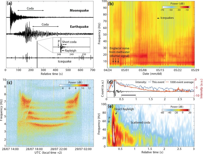
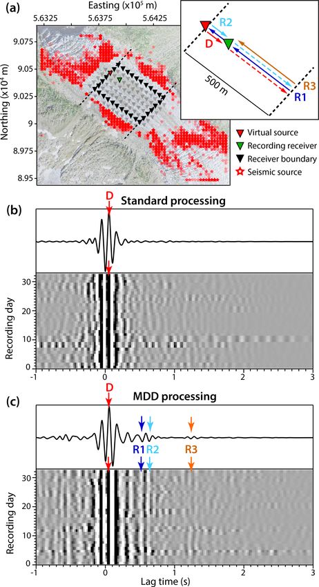
1140                                                          A. Sergeant et al.: Glacier imaging with seismic interferometry

tation have allowed rapid deployments of seismic networks           20 km wide) during a surge, likely due to the switch of the
in remote terrain and harsh polar conditions (Podolskiy and         subglacial drainage from channelized to distributed.
Walter, 2016; Aster and Winberry, 2017). Studies on seismic            The underlying seismic interferometry techniques used in
source processes have revealed unprecedented details about          ambient noise studies are rooted in the fact that the elastic
englacial fracture propagation (e.g. Walter et al., 2009; Mike-     impulse response between two receivers, Green’s function
sell et al., 2012), basal processes (e.g. Winberry et al., 2013;    (GF), can be approximated via cross-correlation of a dif-
Röösli et al., 2016a; Lipovsky et al., 2019), glacier hydrol-       fuse wave field recorded at the two sites (Lobkis and Weaver,
ogy (Bartholomaus et al., 2015; Gimbert et al., 2016), and          2001; Campillo et al., 2014). Seismic interferometry consists
iceberg calving (e.g. Walter et al., 2010; Bartholomaus et al.,     in turning each of the two receivers into a virtual source and
2012; Sergeant et al., 2016, 2018).                                 retrieving the estimated elastic response of the medium at
   The subsurface structure of ice sheets and glaciers has          the other receiver. Under specific assumptions on the source
been characterized by analysis of seismic wave propagation          wave field (see below), the GF estimate is thus expected to
in ice bodies. For example, Harland et al. (2013) and Smith         be symmetric in its causal and acausal portions (referred to
et al. (2017) used records of basal seismicity to measure elas-     as “causal–acausal symmetry”).
tic anisotropy in two Antarctic ice streams. Lindner et al.            In theory, the GF estimate is obtained in media capable of
(2019) identified crevasse-induced anisotropy in an Alpine          hosting an equipartitioned wave field, that is random modes
glacier from velocity anomalies by analyzing icequake seis-         of seismic propagation with the same amount of energy.
mograms at seismic arrays. Walter et al. (2015) used transient      In practice, the equipartition argument has limited applica-
seismic signals generated in moulins to compute frequency-          bility to the Earth because nonhomogeneously distributed
dependent seismic velocities through matched-field process-         sources, in the forms of ambient noise sources, earthquakes,
ing and estimate the depth of the ice-to-bedrock transition         and/or scatterers, prevent the ambient wave field from be-
beneath a seismic network deployed on the Greenland Ice             ing equipartitioned across the entire seismic scale (Fichtner
Sheet (GIS).                                                        et al., 2017, and references therein). The GF estimation from
   At the same time, a new approach appeared in seismol-            inter-station correlation therefore usually relies on simplified
ogy which explores not only earthquakes but also ambi-              approximations of diffusive wave fields which can be reached
ent noise sources generated by climate and ocean activity           in (i) the presence of equally distributed sources around the
(Ekström, 2001; Rhie and Romanowicz, 2004; Webb, 1998;              recording network (Wapenaar, 2004; Gouédard et al., 2008b)
Bonnefoy-Claudet et al., 2006). Shapiro and Campillo (2004)         and/or (ii) in strong-scattering settings as scatterers act like
and Shapiro et al. (2005) pointed out the possibility of using      secondary seismic sources and likely homogenize the ambi-
continuous noise recordings to reconstruct propagating sur-         ent wave field in all incident directions (e.g. Hennino et al.,
face waves across a seismic array and to use them for crustal       2001; Malcolm et al., 2004; Larose et al., 2008). Even if the
tomography in California. Other studies followed, shaping           noise wave field is not generally diffuse (Mulargia, 2012),
the analysis of ambient noise background into a powerful tool       inhomogeneities in the Earth’s crust and the generation of
to constrain the elastic properties of the illuminated medium,      oceanic ambient noise all around Earth make ambient noise
making it possible to image the Earth’s interior from regional      interferometry applications generally successful.
(Yang et al., 2007; Lin et al., 2008) to local scales (e.g. Lin        In glaciers, the commonly used oceanic ambient noise
et al., 2013; Nakata et al., 2015) and monitor seismic fault        field lacks the high frequencies needed to generate GFs that
(e.g. Brenguier et al., 2008b; Olivier et al., 2015) and vol-       contain useful information at the scale of the glacier. To tar-
canic processes (Sens-Schönfelder and Wegler, 2006; Bren-           get shallower glaciers and their bed, we must work with other
guier et al., 2011), for example. Moreover, ambient noise           sources such as nearby icequakes and flowing water which
studies have so far led to original observations such as ther-      excite higher-frequency (> 1 Hz) seismic modes (Sect. 2.1).
mal variations in the subsoil, spatiotemporal evolution of the      In this context, the lack of seismic scattering in homogeneous
water content, and stress changes along fault zones with ap-        ice (Podolskiy and Walter, 2016) renders the reconstruction
plications to geomechanics, hydrology, and natural hazards          of the GF from on-ice recordings challenging. Condition
(Larose et al., 2015).                                              (i) can compensate for lack of condition (ii). However, mi-
   For the cryosphere, few studies have successfully used           croseismicity generated on glaciers is often confined to nar-
oceanic ambient noise at permanent broadband stations de-           row regions such as crevasse margin zones (Roux et al., 2008;
ployed on the rocky margins of glaciers or up to 500 km away        Mikesell et al., 2012) or other water-filled englacial conduits
on polar ice sheets to monitor the subsurface processes. Mor-       (Röösli et al., 2014; Walter et al., 2015; Preiswerk and Wal-
dret et al. (2016) and Toyokuni et al. (2018) tracked the strain    ter, 2018; Lindner et al., 2020). This often prevents the occur-
evolution in the upper 5 km of the Earth’s crust beneath the        rence of homogeneous source distributions on glaciers. Nev-
GIS due to seasonal loading and unloading of the overlaying         ertheless, the abundance of local seismicity indicates a con-
melting ice mass. More recently, Zhan (2019) detected slow-         siderable potential for glacier imaging and monitoring with
ing down of surface wave velocities up to 2 % in the basal till     interferometry.
layer of the largest North American glacier (Bering Glacier,

The Cryosphere, 14, 1139–1171, 2020                                                     www.the-cryosphere.net/14/1139/2020/
A. Sergeant et al.: Glacier imaging with seismic interferometry                                                                 1141

   Few attempts have been conducted on glaciers to obtain           We refer the reader who is not familiar with ambient noise
GF estimates from on-ice seismic recordings. Zhan et al.            seismic processing to the appendix sections providing details
(2013) first calculated ambient noise cross-correlations on         on seismic detection methods, seismic array processing, and
the Amery ice shelf (Antarctica) but could not compute ac-          seismic velocity measurements. Finally, in light of our anal-
curate GF at frequencies below 5 Hz due to the low-velocity         ysis, we discuss suitable array geometries and measurement
water layer below the floating ice shelf, which causes res-         types for future applications of passive seismic imaging and
onance effects and a significantly nondiffusive inhomoge-           monitoring studies on glaciers.
neous noise field. Preiswerk and Walter (2018) successfully
retrieved an accurate GF on two Alpine glaciers from the
cross-correlation of high-frequency (≥ 2 Hz) ambient noise          2     Material and data
seismograms, generated by meltwater flow. However, due
to localized noise sources in the drainage system that also         2.1    Glacier seismic sources
change positions over the course of the melting season, they
could not systematically obtain an accurate coherent GF             Glaciogenic seismic waves couple with the bulk Earth and
when computed for different times, limiting the applications        can be recorded by seismometers deployed at local (Podol-
for glacier monitoring.                                             skiy and Walter, 2016) to global ranges (Ekström et al.,
   As an alternative to continuous ambient noise, Walter et al.     2003). In this study, we focus on three classes of local
(2015) used crevassing icequakes recorded during a 1-month          sources. For an exhaustive inventory of glacier seismicity
seismic deployment at Gornergletscher (Switzerland). They           and associated source mechanisms, we refer to the review
recorded thousands of point source events which offered             papers of Podolskiy and Walter (2016) and Aster and Win-
an idealized spatial source distribution around one pair of         berry (2017).
seismic sensors and could obtain accurate GF estimates. To             Typically on Alpine glaciers and more generally in ab-
overcome the situation of a skewed illumination pattern of-         lation zones, the most abundant class of recorded seismic-
ten arising from icequake locations, Lindner et al. (2018)          ity is related to brittle ice failure which leads to the for-
used multidimensional deconvolution (Wapenaar et al., 2011;         mation of near-surface crevasses (e.g. Neave and Savage,
Weemstra et al., 2017) that relies on a contour of receivers        1970; Mikesell et al., 2012; Röösli et al., 2014; Podolskiy
enclosing the region of interest (see also Sect. 6.2). This         et al., 2019) and the generation of 102 –103 daily recorded
technique proved to be efficient to suppress spurious arrivals      icequakes (Fig. 1a and b). Near-surface icequakes have local
in the cross-correlation function which emerge in the pres-         magnitudes of −1 to 1, and seismic waves propagate a few
ence of heterogeneously distributed sources. However, this          hundred meters before falling below the background noise
method was applied to active sources and synthetic seismo-          level. Icequake waveforms have durations of 0.1–0.2 s and
grams, and its viability still needs to be addressed for passive    thus do not carry much energy at frequencies below 5 Hz
recordings.                                                         (Fig. 1d and e). With its maximum amplitude on the verti-
   In this study, we provide a catalogue of methods to tackle       cal component, Rayleigh waves dominate the seismogram. In
the challenge of applying passive seismic interferometry to         contrast, the prior P-wave arrival is substantially weaker and
glaciers in the absence of significant scattering and/or an         for distant events often below noise level. Rayleigh waves
isotropic source distribution. After a review on glacier seis-      propagate along the surface and are not excited by a source
mic sources (Sect. 2.1), we investigate the GF retrieval on         at depth exceeding one wavelength (Deichmann et al., 2000).
three glacier settings with different patterns of seismic wave      In addition, the crevasse zone is mostly confined to the sur-
fields. In a first ideal case (Glacier d’Argentière in the French   face (≤ 30 m) since ice-overburden pressure inhibits tensile
Alps, Sect. 3), we take advantage of a favorable distribution       fracturing at greater depths (Van der Veen, 1998). That is why
of noise sources and icequakes recorded on a dense array.           such icequakes are usually considered to originate at shallow
In a second case (GIS, Sect. 4), a dominant persistent noise        depth (Walter, 2009; Roux et al., 2010; Mikesell et al., 2012).
source constituted by a moulin prevents the accurate esti-          The short duration and weak seismic coda after the Rayleigh
mate of the GF across the array. We use a recently proposed         wave arrival (compared to earthquake coda propagating in
scheme (Corciulo et al., 2012; Seydoux et al., 2017) that in-       the crust, Fig. 1a; see also further details in Sect. 5.1) are the
volves matched-field processing to remove the moulin signa-         result of limited englacial scattering. This typically allows
ture and improve the GF estimates. In a third case (Gorner-         seismologists to approximate the glacier’s seismic velocity
gletscher in Swiss Alps, Sect. 5), the limited distribution of      model by a homogeneous ice layer on top of a rock half-
icequakes is overcome by the use of crevasse-generated scat-        space when locating events or modeling seismic waveforms
tered coda waves to obtain homogenized diffuse wave fields          (e.g. Walter et al., 2008; Walter et al., 2015).
before conducting cross-correlations. In order to serve as             From spring to the end of summer, another seismic source
a practical scheme for future studies, the three above sections     superimposes on icequake records and takes its origin in flu-
are nearly independent from each other. They focus on the           vial processes. Ice melting and glacier runoff create turbulent
processing schemes to compute or improve the GF estimates.          water flow at the ice surface that interacts with englacial and

www.the-cryosphere.net/14/1139/2020/                                                      The Cryosphere, 14, 1139–1171, 2020
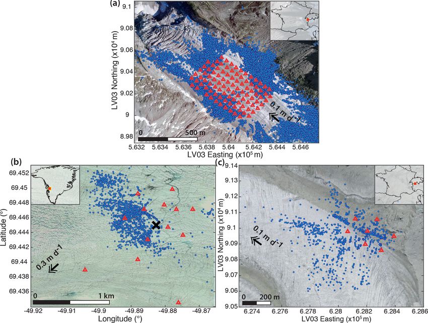
1142                                                              A. Sergeant et al.: Glacier imaging with seismic interferometry

Figure 1. (a) Seismograms of a moonquake, regional earthquake, and typical Alpine glacier seismicity. Moonquake seismogram was recorded
during the 1969–1977 Apollo passive seismic experiment (Nunn, 2017). Zoom on icequake waveform shows the lack of sustained coda in
homogeneous ice when compared to other signals propagating in crustal rocks. (b) Spectrogram of 1 month of continuous recording at Glacier
d’Argentière (French Alps) showing abundance of icequakes (5–100 Hz) and englacial noise (2–30 Hz) produced by turbulent meltwater flow.
(c) Spectrogram for a 10 h long hydraulic tremor produced by the water moulin activity within the Greenland Ice Sheet network (Fig. 2b).
(d) Seismic waveform and associated spectrogram (e) for one icequake recorded at Gornergletscher (Swiss Alps). Color lines in (d) are the
signal intensity (see main text, Sect. 5.1) for this event in blue and averaged over 1000 events in orange (right y axis; note the logarithmic
scale). The horizontal gray bar indicates the coda window which is used to generate the first estimations of Green’s functions (Sect. 5.2).

subglacial linked conduits. Gravity-driven transport of melt-            during peak melt hours. Frequency bands of either elevated
water creates transient forces on the bulk of the Earth (e.g.            or suppressed seismic energy reflect the geometry of the
Schmandt et al., 2013; Gimbert et al., 2014) and surrounding             englacial conduit as it acts as a resonating semi-open pipe,
ice (Gimbert et al., 2016) that generate a mix of body and               modulated by the moulin water level (Röösli et al., 2016b).
surface waves (Lindner et al., 2020; Vore et al., 2019). Melt-              Finally, in Alpine environments, seismic signatures of
water flow noise is recorded continuously at frequencies of              anthropogenic activity generally overlap with glacier am-
1–20 Hz as shown in the 1-month spectrogram of ground ve-                bient noise at frequencies > 1 Hz. Whereas anthropogenic
locity at Glacier d’Argentière (Fig. 1b). Seismic noise power            monochromatic sources can usually be distinguished by their
shows diurnal variations that are correlated with higher dis-            temporal pattern (Preiswerk and Walter, 2018), separation of
charge during daytime and reduced water pressure at night                all active sources recorded on glacier seismograms can prove
(Preiswerk and Walter, 2018; Nanni et al., 2019b).                       difficult. Nevertheless, locating the source regions through
   Englacial and subglacial conduits can also generate acous-            matched-field processing (Corciulo et al., 2012; Chmiel
tic (Gräff et al., 2019) and seismic wave resonances (Röösli             et al., 2015) can help to identify the noise source processes
et al., 2014) known as hydraulic tremors. In the presence                in glaciated environments (Sect. 4).
of moulin, water flowing to the glacier base creates seismic
tremors (Fig. 1c) which often dominate the ambient noise

The Cryosphere, 14, 1139–1171, 2020                                                            www.the-cryosphere.net/14/1139/2020/
A. Sergeant et al.: Glacier imaging with seismic interferometry                                                                    1143

Figure 2. Icequake locations (blue dots) and seismic stations (red triangles) superimposed on aerial photographs of (a) Argentière (© IGN
France), (b) the Greenland Ice Sheet (© Google, Mixar Technologies), and (c) Gornergletscher (© swisstopo, SWISSIMAGE). The black
arrows indicate ice flow direction. Black cross in (b) indicates the location of the moulin within the array.

2.2   Study sites and seismic experiments                              2.2.1   Glacier d’Argentière array

We use seismic recordings from three seasonally deployed
networks in the ablation zones of two temperate Alpine                 The Argentière seismic array (Fig. 2a) was deployed in late
glaciers and of the GIS. Each of the acquired datasets                 April 2018 and recorded for 5 weeks. It consists of 98 three-
presents different patterns of seismic wave fields correspond-         component surface sensors regularly spaced on a grid with
ing to the three configurations investigated for GF esti-              a 350 m × 480 m aperture and a station-to-station spacing of
mate retrieval, as defined in the introduction. All networks           ∼ 40 m for the along-flow profiles and ∼ 50 m for the across-
recorded varying numbers of near-surface icequakes (blue               flow profiles. This large N-array experiment used the tech-
dots in Fig. 2a–c). Different processing schemes were used             nology of nodes (Fairfield Nodal ZLand 3C) that combine
to constitute the icequake catalogues and are detailed in Ap-          a geophone, digitizer, battery, data storage, and GPS in a sin-
pendix A. In this study we only use vertical component                 gle box (Hand, 2014) and allowed a rapid deployment within
data of ground velocity to generate vertical-to-vertical cross-        a few hours. ZLand geophones have a natural frequency of
correlation functions which primarily contain the Rayleigh             5 Hz and recorded continuously at a sampling rate of 500 Hz.
wave fundamental mode (Shapiro and Campillo, 2004).                    Besides seismic sensors, four on-ice GPS instruments were
Some of the datasets involve surface seismometers whose                deployed. At the array site, the ice is 80–260 m thick (Hantz,
horizontal components are regularly shifted over the course            1981) and flows at an approximate rate of 0.1 m d−1 . The sen-
of the melting season. Obtaining GF estimates from horizon-            sors were placed about 30 cm into the snow and accumulated
tal component data requires additional preprocessing to ob-            about 4 m of downstream displacement at the end of the ex-
tain accurate orientations of the seismic sensors.                     periment. Because of snowmelt, we had to level and reorient
                                                                       the instruments twice during the experiment. A digital eleva-
                                                                       tion model (DEM) for the glacier bed was obtained using 14

www.the-cryosphere.net/14/1139/2020/                                                         The Cryosphere, 14, 1139–1171, 2020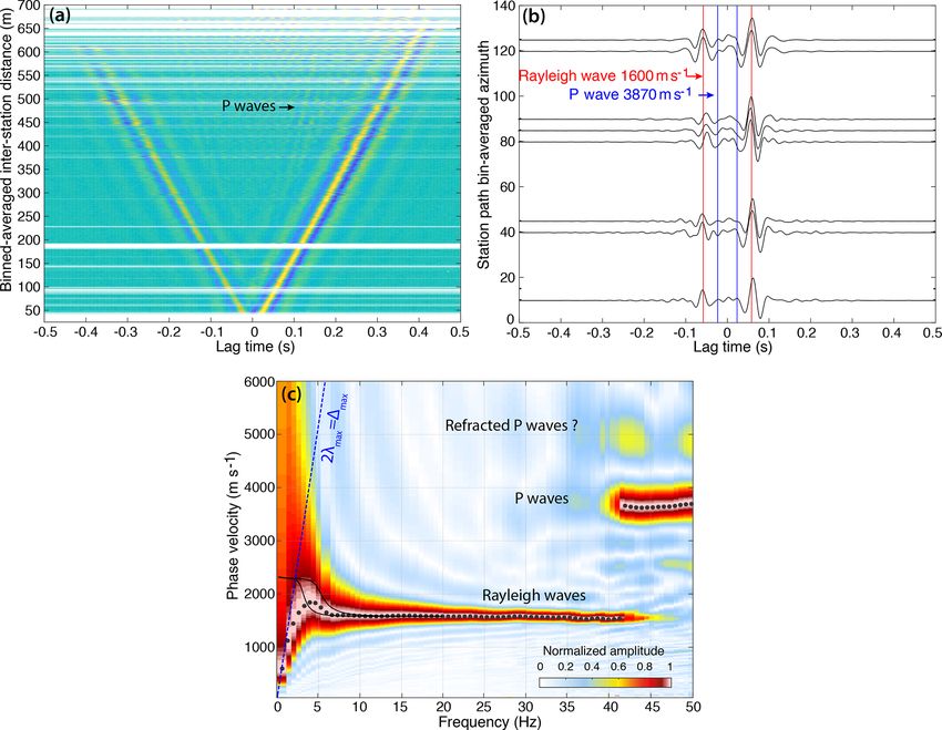
1144                                                          A. Sergeant et al.: Glacier imaging with seismic interferometry

ground-penetrating radar tracks over the area covered by the        When stacking the individual ICC on all events, only the
seismic array, and a glacier surface DEM was acquired from          sources that lie in the stationary phase zones, i.e. aligned
a drone survey.                                                     with the two-receiver direction, actually contribute to the GF
                                                                    (Gouédard et al., 2008b). The aperture of the stationary phase
2.2.2   Greenland Ice Sheet array                                   zones, also called “the endfire lobes” (Fig. B4a), depends
                                                                    on the considered seismic wavelength (Roux et al., 2004).
The GIS network (Fig. 2b) was deployed 30 km north of the           In the case of anisotropic source distribution, the contribu-
calving front of the Jakobshavn Isbræ from 2 July to 17 Au-         tion of nonstationary sources eventually does not vanish and
gust 2011. The details of the study site and the seismic net-       gives rise to spurious arrivals in the final GF estimate. Prior
work can be found in Röösli et al. (2014), Ryser et al. (2014),     to stacking, we assign all cross-correlations to event azimuth
and Andrews et al. (2014). We use seismic recordings from           bins of 5◦ to attribute equal weights to all incident directions.
13 stations: 12 seismometers (1 Hz Lennartz) installed on the       To reduce eventual spurious arrivals, we compute the GF on
surface or shallow boreholes (2–3 m deep), and one surface          selected sources in the endfire lobes whose aperture is calcu-
broadband seismometer (Trillium Compact 120 s corner pe-            lated for maximum wavelengths corresponding to 3 Hz (Ap-
riod). Seismometers recorded continuously with a sampling           pendix B3).
frequency of 500 Hz. The array has a 1.8 km aperture. It is            For noise cross-correlation (NCC), we use a similar proto-
located around a prominent moulin with an average intake of         col as the one of Preiswerk and Walter (2018). To reduce the
2.5 m3 s−1 of meltwater. At the study site, the ice is approx-      effects of teleseismic events or the strongest icequakes, we
imately 600 m thick and flows at ∼ 0.3 m d−1 (Röösli et al.,        disregard the seismic amplitudes completely and consider 1-
2016a).                                                             bit normalized seismograms (Bensen et al., 2007). By doing
                                                                    so, we attribute a similar weight to ambient noise and ice-
2.2.3   Gornergletscher array
                                                                    quake source contributions to the GF. The traces are cross-
The Gornergletscher network (Fig. 2c) operated between              correlated in nonoverlapping 30 min long windows. Result-
28 May and 22 July 2007. It consists of seven seismome-             ing NCCs are stacked daily and then averaged over the 5
ters (six 8 Hz Geospace 11D and one 28 Hz Geospace 20D)             weeks of recording. We finally obtain a set of 4371 NCCs
installed in shallow boreholes (2–3 m deep). They recorded          that corresponds to the GF estimates for all combinations of
continuously with a sampling frequency of 1000 Hz. The ar-          sensor pairs.
ray has a 320 m aperture. At the study site, the ice is approx-
imately 160 m thick and flows at ∼ 0.1 m d−1 (Walter, 2009).        3.1   Green’s function estimates

                                                                    Figure 3a shows the stacked section of NCCs averaged in
3   Passive interferometry at the Glacier d’Argentière              1 m binned distance intervals. Coherent Rayleigh waves with
    dense array                                                     propagation velocity of 1600 m s−1 are well reconstructed
                                                                    across the array. We also observe emergence of weak but
We use a standardized processing scheme for computing GF            faster waves identified at higher frequencies as P waves trav-
estimates here. We either cross-correlate seismogram time           eling in the ice.
windows, which encompass ballistic seismic waves of the                Slight disparities in amplitudes of the causal and acausal
icequake catalogue, or cross-correlate continuous seismo-           parts of the GF estimates (positive versus negative times) are
grams as traditionally done in ambient noise studies. Prior to      related to the noise source density and distribution. Higher
any calculation, seismic records are corrected for instrumen-       acausal amplitudes observed at larger distances are evidence
tal response and converted to ground velocity. Seismograms          for a higher density of sources located downstream of the
are then spectrally whitened between 1 and 50 Hz because of         array, according to our cross-correlation definition. More
low instrumental sensitivity at lower frequency.                    sources downstream are likely generated by faster water flow
   For icequake cross-correlation (ICC), we follow the              running into subglacial conduits toward the glacier icefall
method of Gouédard et al. (2008b) and Walter et al. (2015)          (Gimbert et al., 2016; Nanni et al., 2019b). Looking closer
on 11.1 × 10³ events. The length of the correlation window          at NCC for individual receiver pairs, we sometimes observe
T is adjusted to the nature of seismic sources and the ar-          spurious arrivals around time 0 (marked as green dots in
ray aperture. Here we use T = 0.5 s given the short icequake        Fig. 3b), mostly at station pairs oriented perpendicular to the
duration and the maximum station separation of 690 m. To            glacier flow (i.e. azimuth 0◦ ≤ φ ≤ 50◦ ), indicating that dom-
avoid near-field source effects and to account for near-planar      inant noise sources are located along the flow line. At other
wave fronts, we select events that lie outside a circle centered    station pairs (i.e. azimuth φ ∼ 90◦ ), the reconstructed arrival
at the midpoint between the two considered stations and with        times are slightly faster than expected. This could be an ef-
a radius equal to the inter-station distance (Fig. B4a). The        fect of non-distributed noise sources and/or anisotropy intro-
plane wave approximation implies a sinusoidal dependence            duced by englacial features (Sect. 3.3). This analysis shows
of the arrival times with respect to event azimuth (Fig. B4b).      that even if the noise sources are not equally distributed in

The Cryosphere, 14, 1139–1171, 2020                                                     www.the-cryosphere.net/14/1139/2020/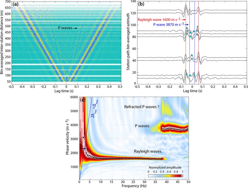
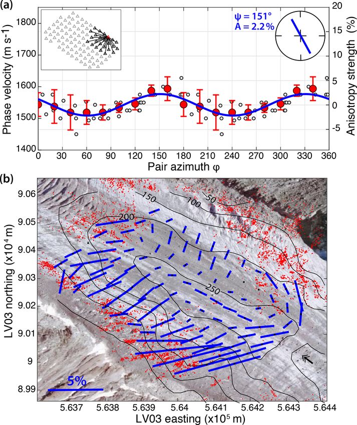
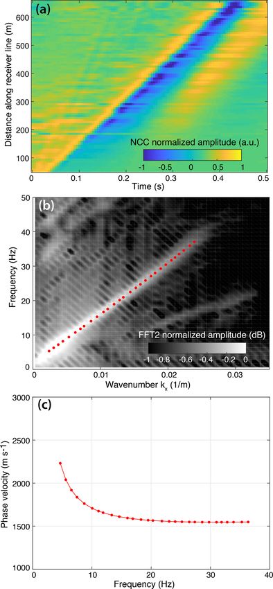
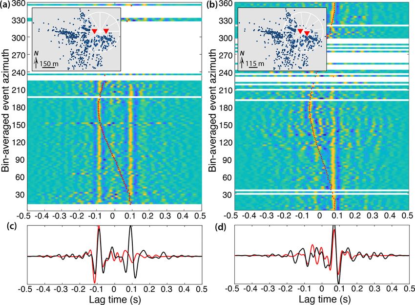
A. Sergeant et al.: Glacier imaging with seismic interferometry                                                                           1145

Figure 3. (a) Noise cross-correlations (NCCs) sorted by increasing inter-station distances at Glacier d’Argentière. For the representation,
correlation functions are averaged in 1 m distance bins and band-pass filtered between 10 and 50 Hz to highlight the presence of high-
frequency P waves. (b) Azimuthal dependence of GF estimates for pairs of stations 100 m apart. Accurate GF estimates are obtained at station
paths roughly aligned with the glacier flow (azimuth ∼ 120◦ ), indicating more noise sources likely located downstream and upstream of the
array. For other station paths, we observe spurious arrivals (indicated by green dots) before the expected arrival times for Rayleigh (red bars)
and P waves (blue bars) which primarily arise from non-distributed noise sources that lie outside the stationary phase zones of these stations
(see main text). (c) Frequency–velocity diagram obtained from f-k (frequency–wavenumber) analysis of NCC in (a). The dispersion curve
of phase velocity for Rayleigh waves and P waves is plotted as black dots. The dashed blue line shows the frequency-dependent resolution
limit, given the maximum wavelength and sensor spacing λmax = 1max /2. Black lines are theoretical dispersion curves for fundamental
mode Rayleigh wave velocity computed for ice thickness of either 150 or 250 m with Geopsy software. We used the elastic parameters
for the ice and bedrock as given in Preiswerk and Walter (2018, Sect. 6.1). The same figure for icequake cross-correlations is available in
Appendix (Fig. B2).

space, averaging the NCC in regular distance intervals on                    Seismic phases and their velocities can be identified on
a dense array deployment helps the GF estimate convergence.               the frequency–velocity diagram (Fig. 3c, black dots) that
   The stacked section of ICCs (Fig. B2a) yields similar re-              is obtained from frequency–wavenumber (f-k) analysis of
sults to those of the NCC (Fig. 3a). The control of the ice-              the NCC computed on a line of receivers (Appendix B1).
quake source aperture enables us to minimize the spurious                 As identified above, the correlation functions reconstruct
arrivals which are observed on some NCC (Fig. 3b) and ob-                 P waves traveling in the ice well with an average velocity
tain more accurate Rayleigh wave travel times at most sta-                Vp = 3870 m s−1 . We also observe weak intensity but fast
tion paths (Fig. B2b). The differences in ICC and NCC sup-                seismic phases at frequencies above 35 Hz, which could cor-
port that NCCs are more sensitive to the noise sources rather             respond to refracted P waves traveling along the basal inter-
than icequake sources. Icequake contributions certainly en-               face with a velocity around 5000 m s−1 .
able us to widen the spectral content of the NCC to frequen-                 Surface waves are dispersive, meaning that their veloc-
cies higher than 20 Hz, as the most energetic ambient noise               ity is frequency-dependent, with higher frequencies being
is recorded in the 1–20 Hz frequency band (Fig. 1b).                      sensitive to surface layers and conversely lower frequen-

www.the-cryosphere.net/14/1139/2020/                                                              The Cryosphere, 14, 1139–1171, 2020
1146                                                        A. Sergeant et al.: Glacier imaging with seismic interferometry

cies being sensitive to basal layers. Theoretical dispersion
curves for Rayleigh wave fundamental mode are indicated as
black solid lines in Fig. 3c. They correspond to a two-layer
model with the top ice layer of thickness H = 150 m and
H = 250 m over a semi-half-space representing the bedrock.
The dashed blue line indicates the array resolution capa-
bility that corresponds to the maximum wavelength limit
λmax = 1max /2 (Wathelet et al., 2008), with 1max being the
maximum sensor spacing. Reconstruction of Rayleigh waves
and resolution of their phase velocities using f-k processing
are differently sensitive for NCC and ICC at frequencies be-
low 5 Hz (Fig. 3c versus Fig. B2c) as ICCs have limited en-
ergy at low frequency (Fig. 4a) due to the short and impulsive
nature of icequake seismograms (Fig. 1d and e). Given the
vertical sensitivity kernels for Rayleigh wave phase velocity
(Fig. 4b) and the dispersion curves obtained from the cross-
correlation sections (Figs. 3c and B2c), Rayleigh waves that
are reconstructed with NCC are capable of sampling basal ice
layers and bedrock while ICCs are more accurately sensitive
to the ice surface. These results reflect the S-wave velocity
dependence on depth.

3.2    Dispersion curve inversion and glacier thickness           Figure 4. (a) Probability density function of noise cross-correlation
       estimation                                                 (NCC) spectra (colors) and median average of icequake cross-
                                                                  correlation (ICC) spectra (black line). Note that raw data (i.e con-
Sensitivity of Rayleigh waves obtained on NCC to frequen-         tinuous noise or icequake waveforms) were spectrally whitened be-
cies below 5 Hz enables us to explore the subsurface struc-       tween 1 and 50 Hz prior to cross-correlation. Due to spectral content
                                                                  of englacial noise and icequakes, NCCs and ICCs have different
ture with inversions of velocity dispersion curves. Due to the
                                                                  depth sensitivity due to spectral response. (b) Vertical sensitivity
general noise source locations up-flow and down-flow of the       kernels for phase velocities of the Rayleigh wave a fundamental
network, we limit our analysis to receiver pairs whose accu-      mode for an ice thickness of 200 m over a semi-half-space repre-
rate GF could be obtained. We thus compute the dispersion         senting the bedrock. The kernels were computed using the freely
curves on eight along-flow receiver lines which constitute the    available code of Haney and Tsai (2017).
array (inset map in Fig. 5). For each line, we invert the 1-D
ground profile which best matches seismic velocity measure-
ments in the 3–20 Hz frequency range, using the neighbor-         version resolves the S-wave velocity in the ice layer well as
hood algorithm encoded in the Geopsy software (Wathelet,          all best matching models yield to Vs = 1707 m s−1 for mis-
2008).                                                            fit values below 0.05, meaning that the data dispersion curve
   Following Walter et al. (2015), we assume a two-layer          is adjusted with an approximate error below 5 %. The best-
medium consisting of ice and granite bedrock. This is a sim-      fitting model gives a 236 m thick ice layer and bedrock S ve-
plified approximation and does not include 2-D and 3-             locity of 2517 m s−1 . Walter et al. (2015) explored the sensi-
D effects and anisotropy introduced by englacial features         tivity of the basal layer depth to the other model parameters
(Sect. 3.3). The grid search boundaries for seismic veloc-        and reported a trade-off leading to an increase in inverted
ity, ice thickness, and density are given in Table 1. We fix      ice thickness when increasing both ice and bedrock veloci-
the seismic P-velocity in ice to 3870 m s−1 as measured in        ties. Here the ice thickness estimation is most influenced by
Fig. 3c and couple all varying parameters to the S-wave ve-       the rock velocities as we notice that a 100 m s−1 increase in
locity structure with the imposed condition of increasing ve-     basal S velocity results in an increase in ice thickness up to
locity with depth.                                                15 m. These results are moreover influenced by larger uncer-
   Figure 5a and b show the inversion results for the receiver    tainties at lower frequencies (Fig. 5a), which comes from less
line at the center of the array labeled “4”. Velocity mea-        redundant measurements at large distances. Furthermore, 3-
surements are indicated by yellow squares, and dispersion         D effects could lead to some errors in the depth inversion
curves corresponding to explored velocity models are in col-      results which need to be further investigated.
ors sorted by misfit values. Misfit values correspond here to         From the eight receiver line inversions, we find average
the root-mean-square error on the dispersion curve residu-        S-wave velocities of 1710 m s−1 for the ice and 2570 m s−1
als, normalized by the uncertainty average we obtained from       for the granite and a P-wave velocity of 4850 m s−1 in the
the seismic data extraction (error bars in Fig. 5a). The in-      basement, which is consistent with our measurement for re-

The Cryosphere, 14, 1139–1171, 2020                                                     www.the-cryosphere.net/14/1139/2020/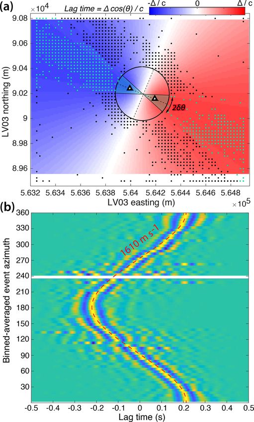
A. Sergeant et al.: Glacier imaging with seismic interferometry                                                                             1147

Figure 5. Inversion of glacier thickness using velocity dispersion curves of Rayleigh waves and the Geopsy neighborhood algorithm. Disper-
sion curve measurements are obtained from f-k analysis of noise cross-correlations on eight receiver lines whose geometry is described in the
bottom-right panel. (a, b) Color-coded population of (a) dispersion curve fits and (b) S-wave velocity profiles for the node along-flow line
labeled 4 in (c). Warmer colors correspond to smaller misfit, and gray lines correspond to models with misfit values higher than 0.1. In (a) the
dispersion curve and uncertainties obtained from seismic measurements are overlaid in yellow squares. For comparison, the dispersion curve
computed for the node line 7 and associated with a thinner ice layer is plotted in white dots. (c) Across-flow profile of (red line) ice thickness
estimates from Rayleigh wave velocities obtained at eight along-flow node lines and (black line) average basal topography from a DEM.
Dashed blue zones indicate the presence of a low P-velocity top layer from seismic inversions. Uncertainties in ice thickness estimates (red
error bars) correspond to seismic inversion results which yield to a misfit lower than 1 standard deviation of misfit values from the 2500
best-fitting models. Black dashed lines indicate deviations from the glacier baseline around each node line due to longitudinal topography
gradients.

fracted P waves in Fig. 3c. Vp /Vs ratios are found to be 2.2              pronounced transversal crevasses (i.e. perpendicular to the
and 1.9 for ice and granite, giving Poisson’s ratios of 0.37 and           receiver lines; see Sect. 3.3) near the array edges, which do
0.3, respectively. For the receiver lines near the array edges             not extend deeper than a few dozens of meters (Van der Veen,
(lines 1–3 and 8), the inversion yields to a low P-velocity sur-           1998) and can be modeled as a slow layer above faster ice
face layer of 15 and 7 m thickness, respectively, above thicker            (Lindner et al., 2019).
ice (dashed blue zone in Fig. 5c). In this thin top layer, the                Inversion results for the ice thickness are plotted in red in
matching S velocity corresponds to the one for the ice (i.e.               Fig. 5c. Associated uncertainties (red error bars) are given
1710 m s−1 ). The Vp /Vs ratio is around 1.6 and corresponds               by the models which fit the dispersion curves with misfit val-
to a Poisson’s ratio of 0.2. This is what is expected for snow,            ues below 1 standard deviation of the 2500 best-fitting mod-
although only a ∼ 5 m snow cover was present in the area at                els. The errors on the basal interface depth generally corre-
the time of the experiment. This low-velocity surface layer                spond to a maximum misfit value of 0.02. The black solid
could also at least be partially attributed to the presence of             line shows the across-flow profile of the glacier baseline,

www.the-cryosphere.net/14/1139/2020/                                                               The Cryosphere, 14, 1139–1171, 2020
1148                                                          A. Sergeant et al.: Glacier imaging with seismic interferometry

which was extracted from the DEM of Glacier d’Argentière
(Sect. 2.2.1) and averaged over the geophone positions. Re-
sults show that ambient noise interferometry determines the
depth of the basal interface with a vertical resolution of 10 m,
equivalent to ∼ 5 % accuracy relative to the average depth, as
we are able to reproduce the transverse variations in the ice
thickness. Differences in ice thickness values between our
measurements and the DEM are generally less than 20 m (the
DEM resolution), and the maximum error is 35 m for line 3.
   Errors and uncertainties on mapping the basal interface are
primarily linked to bedrock velocities, as discussed above.
Potentially, the bed properties can be refined using additional
measurements from refracted P waves that should be recon-
structed on NCC obtained on such a dense and large array
and stacked over longer times. Ice thickness estimation is
also affected by 2-D and 3-D effects as phase velocities are
averaged here over multiple receiver pairs. The confidence
interval we obtain for basal depth is of a similar order to the
actual variations in glacier thickness along the receiver lines
(black dashed lines). More accurate 3-D seismic models of
the glacier subsurface could be obtained using additional sta-
tion pairs as discussed in Sect. 6.

3.3    Azimuthal anisotropy from average phase velocities
                                                                    Figure 6. (a) Azimuthal variation in phase velocities measured at
Smith and Dahlen (1973) show that for a slightly anisotropic
                                                                    one node (red triangle in the inset map). White dots are the phase
medium the velocity of surface waves varies in 2φ-azimuthal         velocity measurements obtained for different azimuths φ that are
dependence according to                                             defined by the station pair orientation. To avoid spatial averaging,
                                                                    we only consider subarrays of 250 m aperture around the target node
c(φ) = c0 + A cos[2(φ − ψ)],                                (1)     at the center as described by black triangles in the inset map. Red
                                                                    dots are phase velocities averaged in 20◦ azimuth bins. The thick
where c0 is the isotropic component of the phase velocity, A        blue curve is the best fit for the 2φ azimuthal variation in the aver-
is the amplitude of anisotropy, and ψ defines the orientation       aged velocity measurements in red. Fast-axis angle and anisotropy
of the anisotropic fast axis. On glaciers, azimuthal anisotropy     strength are indicated in the top right corner circle. (b) Map of fast-
                                                                    axis direction and amplitude of anisotropy measured at 25 Hz, su-
can be induced by englacial crevasses, with fast direction for
                                                                    perimposed on an orthophotograph (© IGN France). Locations of
Rayleigh wave propagation being expected to orient paral-
                                                                    icequakes active for 7 d are plotted in red dots to highlight the ori-
lel to the crack alignment (Lindner et al., 2019). Glacier and      entations of surface crevasses. Basal topography contour lines are
ice sheets are also represented as transversely isotropic me-       indicated every 50 m. The black arrow indicates ice flow direction.
dia whose type of symmetry depends on the ice fabric (e.g.
Diez and Eisen, 2015; Horgan et al., 2011; Smith et al., 2017;
Picotti et al., 2015).
   The dense array experiment of Glacier d’Argentière cov-             For each sensor position, we obtain c velocity measure-
ers a wide range of azimuths φ defined by the orientation of        ments as a function of the φ-azimuth of the receiver pair that
the station pairs and allows us to investigate azimuthal varia-     includes the target station. To reduce the effect of spatial av-
tion in Rayleigh wave velocities at any given sensor. In order      eraging, we compute anisotropy parameters ψ and A consid-
to cover a maximum range of φ-azimuth, we compute ve-               ering subarrays of stations that lie within 250 m of the target
locity dispersion curves for Rayleigh waves obtained for the        point (inset map in Fig. 6a). ψ and A values are found at each
correlation functions computed on icequake signals (ICCs),          station cell by fitting c(φ) with Eq. (1) using a Monte Carlo
since accurate GF estimates from ambient noise are limited          inversion scheme. Note that the formulation of Eq. (1) also
to station pair directions with azimuth φ roughly aligned with      gives rise to an additional 4φ dependence of velocities. Lind-
ice flow (φ ∼ 120◦ , Sect. 3.1). To measure phase velocities at     ner et al. (2019) used a beam-forming approach on icequake
different frequencies, we apply a slant-stack technique sim-        records at 100 m aperture arrays and found that adding the
ilar to that of Walter et al. (2015) to octave-wide frequency       4φ component to describe the azimuthal variations in phase
ranges by band-pass filtering the individual ICC, at each sta-      velocities induced by glacier crevasses yields similar ψ and
tion pair (Appendix B3).                                            A. We therefore neglect the 4φ term in the present analysis.

The Cryosphere, 14, 1139–1171, 2020                                                       www.the-cryosphere.net/14/1139/2020/
A. Sergeant et al.: Glacier imaging with seismic interferometry 1149
Table 1. Parameter ranges and fixed parameters for grid search to invert the dispersion curves in Fig. 5 for ice thickness. Poisson’s ratios of ice
and granite were varied between 0.2 and 0.5. Poisson’s ratio, ice thickness, and P-wave velocity Vp were coupled to the S-wave velocity Vs .
Material Thickness (m) Vp (m s−1 ) Vs (m s−1 ) Density (kg m−3 )
Ice 50–500 3870 (fixed) 1500–2100 917 (fixed)
Granite ∞ 3870–6000 1500–3500 2750 (fixed)
Anisotropy is observed to be more pronounced near the in terms of crevasse extent and depth of the anisotropic layer
glacier margins (lines 1–2 and 8 as labeled in Fig. 5c), where or any other cause for the observed patterns.
the anisotropy strength varies between 2 % and 8 % (Fig. 6b).
There, fast-axis directions of Rayleigh wave propagation co-
incide with the observed surface strike of the ice-marginal 4 Matched-field processing of englacial ambient
crevasses that are also responsible for the generation of seismic noise
icequakes indicated by red dots. At other locations, fast-
As pointed out earlier, localized englacial noise sources re-
axis directions indicate the presence of transversal crevasses
lated to water drainage can prevent the reconstruction of sta-
(i.e. perpendicular to the ice flow) with weaker degrees of
ble GF estimates by introducing spurious arrivals (i.e. Walter,
anisotropy up to 4 %. While the near-surface crevasses ob-
2009; Zhan et al., 2013; Preiswerk and Walter, 2018). In this
served at the array edges result from shear stress from the
case, the workflow processing traditionally used in the NCC
margin of the glacier, the transversal crevasses are formed
procedure as presented in Bensen et al. (2007) and Sect. 3 is
by longitudinal compressing stress from lateral extension of
not sufficient. Accordingly, we need to apply more advanced
the ice away from the valley side walls, which is typical for
processing methods that can reduce the influence of local-
glacier flow dynamics in ablating areas (Nye, 1952).
ized sources and enhance a more isotropic distribution of the
Alignment of the fast-axis directions with that of ice flow
ambient sources around receiver pairs.
appears along the central lines of the glacier (receiver lines
One of the approaches we apply here is matched-field
4–5) with anisotropy degrees of 0.5 % to 1.5 %. This feature
processing (MFP) (Kuperman and Turek, 1997), which is
is only observed along the deepest part of the glacier where it
an array processing technique allowing the location of low-
flows over a basal depression. Results are here computed for
amplitude sources. MFP is similar to traditional beam form-
seismic measurements at 25 Hz, and maps of anisotropy do
ing that is based on phase-delay measurements. MFP was
not change significantly with frequency over the 15–30 Hz
used for location and separation of different noise sources
range. If we extend our analysis down to 7 Hz, we notice that
in various applications, i.e., to monitor geyser activity (Cros
the aligned-flow fast-axis pattern starts to become visible at
et al., 2011; Vandemeulebrouck et al., 2013), in an explo-
10 Hz. At frequencies lower than 10 Hz, the fast-axis gener-
ration context (Chmiel et al., 2016), and in geothermal field
ally tends to align perpendicular to the glacier flow because
(Wang et al., 2012) and fault zone (Gradon et al., 2019) event
lateral topographic gradients introduce 3-D effects and non-
detection. MFP was also used by Walter et al. (2015) to mea-
physical anisotropy. The results presented here are not punc-
sure phase velocities of moulin tremor signals on the GIS.
tual measurements but are rather averaged over the entire ice
Moreover, joint use of MFP and the singular value decom-
column. The vertical sensitivity kernels for Rayleigh waves
position (SVD) of the cross-spectral density matrix allows
(Fig. 4b) are not zero in the basal ice layers at the consid-
the separation of different noise source contributions, as in
ered frequencies. The align-flow anisotropic pattern is likely
multi-rate adaptive beam forming (MRABF: Cox, 2000). The
attributed to a thin water-filled conduit at depth, as also sug-
SVD approach was explored by Corciulo et al. (2012) to lo-
gested by locations of seismic hydraulic tremors at the study
cate weak-amplitude subsurface sources, and Chmiel et al.
site (Nanni et al., 2019a).
(2015) used it for microseismic data denoising. Also, Sey-
Generally, we observe an increase in the degree of
doux et al. (2017) and Moreau et al. (2017) showed that the
anisotropy with frequency, which is evident for a shal-
SVD-based approach improves the convergence of NCC to-
low anisotropic layer. Conversely, an increase in anisotropy
wards the GF estimate. Here, we combine MFP and SVD
strength at lower frequency would indicate a deeper
in order to remove spurious arrivals in NCC caused by the
anisotropic layer. At the Alpine plateau Glacier de la Plaine
moulin located within the GIS array and thus improve the
Morte, Lindner et al. (2019) find azimuthal anisotropy at fre-
GF estimate emergence.
quencies of 15–30 Hz with strength up to 8 %. They also
find that constraining the depth of the anisotropy layer is not
straightforward as there exists a trade-off between its thick-
ness and the degree of anisotropy. Without any further mod-
eling effort, we refrain from further interpreting our results
www.the-cryosphere.net/14/1139/2020/ The Cryosphere, 14, 1139–1171, 20201150 A. Sergeant et al.: Glacier imaging with seismic interferometry
4.1 Location of noise sources at the GIS via ber of independent parameters that can be used to describe
matched-field processing the wave field in the chosen basis of functions. This number
depends on the analyzed frequency, slowness of the medium
Röösli et al. (2014) and Walter et al. (2015) documented the (inverse of velocity), and average inter-station spacing of the
presence of hour-long tremor signals in GIS seismic records, array (here 736 m). The higher frequency bound (6 Hz) en-
typically starting in the afternoon hours. These events oc- sures no spatial aliasing in the beam-former output, given the
curred on 29 d out of the 45 d total monitoring period. Sig- minimum sensor spacing of 156 m.
nal intensity and duration depended on the days of observa- Figure 7a shows the grid search for MFP performed over
tions, and the energy was mostly concentrated in the 2–10 Hz easting and northing positions. In order to reveal the loca-
range within distinct frequency bands (Fig. 1b). Röösli et al. tion of the source, we use the Bartlett processor (Baggeroer
(2014) and Röösli et al. (2016b) showed a clear correlation et al., 1993) to measure the match between the recorded and
between water level in the moulin and start and end times modeled wave field. The MFP output reveals two dominant
of the tremor; therefore the tremor signal is referred to as noise sources: a well-constrained focal spot corresponding to
“moulin tremor”. Figure 1c shows a spectrogram of a moulin the moulin position inside the GIS array and another source
tremor lasting for 10 h on the night of 28–29 July 2011 and located north of the array. The latter source is revealed by
recorded at one station located 600 m away from the moulin. a hyperbolic shape. This shape is related to a poor radial res-
This signal is generated by the water resonance in the moulin, olution of the beam former for sources located outside of
is coherent over the entire array, and dominates the ambient an array. Walter et al. (2015) suggested that this dominant
noise wave field during peak melt hours (Röösli et al., 2014; source might correspond to another moulin as satellite im-
Walter et al., 2015). agery shows the presence of several drainage features north
We briefly summarize the basics of MFP, and the details of the array. Both noise source signals contribute to the NCC.
of the method can be found in Cros et al. (2011), Walter However, while the source located outside of the array con-
et al. (2015), and Chmiel et al. (2016). MFP exploits the tributes to the stationary-phase zone (endfire lobes) of cer-
phase coherence of seismic signals recorded across an ar- tain receiver pairs, the moulin located within the array will
ray. It is based on the match between the cross-spectral den- mostly cause spurious arrivals on NCC. In order to separate
sity matrix (CSDM) and a modeled GF. The CSDM captures the contribution of these noise sources, we first perform SVD
the relative phase difference between the sensors, as it is the of the CSDM, and then we use a selection of eigenvectors and
frequency-domain equivalent of the time-domain correlation eigenspectral equalization (Seydoux et al., 2017) to improve
of the recorded data. The CSDM is a square matrix with the convergence of NCC towards an estimate of the GF.
a size equivalent to the number (N = 13 for the GIS array) of
stations (N-by-N matrix). MFP is a forward propagation pro- 4.2 Green’s function estimate from eigenspectral
cess. It places a “trial source” at each point of a search grid, equalization
computes the model-based GF on the receiver array, and then
calculates the phase match between the frequency-domain- SVD is a decomposition of the CSDM that projects the max-
modeled GF and the Fourier transform of time-windowed imum signal energy into independent coefficients (i.e. Moo-
data. The optimal noise source location is revealed by the nen et al., 1992; Konda and Nakamura, 2009; Sadek, 2012).
grid points with maximum signal coherence across the array. It allows the split of the recorded wave field into a set of
In order to calculate the MFP output, we use 24 h data linearly independent eigencomponents, each of them corre-
of continuous recordings on 27 July which encompass the sponding to the principal direction of incoming coherent en-
moulin tremor. We calculate a daily estimate of the CSDM ergy and bearing its own seismic energy contribution:
by using 5 min long time segments in the frequency band be- N
X N
X
tween 2.5 and 6 Hz, which gives in total M = 288 of seg- K = U SV T = Ki = Ui 0i ViT , (2)
ments for 1 d. This ensures a robust, full-rank estimation i=1 i=1
of the CSDM (M
N). The modeled GFs are computed where K is the CSDM, N is the number of receivers, U
over the two horizontal spatial components (easting and nor- and V are unitary matrices containing the eigenvectors, and
thing) using a previously optimized Rayleigh wave veloc- S is a diagonal matrix representing the eigenvalues 0, and
ity of c = 1680 m s−1 corresponding to the propagation of T denotes the transpose of the matrix. The total number of
Rayleigh waves within the array obtained by Walter et al. eigenvalues corresponds to the number N of receivers. The
(2015). The MFP output is averaged over 30 discrete fre- CSDM can be represented as the arithmetic mean of individ-
quencies in the 2.5–6 Hz range. ual CSDMs (Ki ), where each Ki is a CSDM corresponding
The lower frequency bound (2.5 Hz) ensures a higher rank to a given singular value 0i .
regime of the seismic wave field, as defined in Seydoux et al. The SVD separates the wave field into dominant (coher-
(2017). It means that the degree of freedom of the seismic ent) and subdominant (incoherent) subspaces. It has been
wave field is higher than the number of stations. The degree shown that the incoherent sources correspond to the small-
of freedom of the seismic wave field is defined as a num- est eigenvalues (Bienvenu and Kopp, 1980; Wax and Kailath,
The Cryosphere, 14, 1139–1171, 2020 www.the-cryosphere.net/14/1139/2020/A. Sergeant et al.: Glacier imaging with seismic interferometry 1151
Figure 7. (a) Location of the dominant noise sources using MFP in the frequency band between 2.5 and 6 Hz (the MFP output is averaged
over 30 discrete frequencies). The MFP was calculated using daily data recorded on 27 July at the 13 presented stations (black triangles).
Blue cross indicates the moulin position. (b) Eigenvalue distribution of the CSDM for 30 discrete frequencies in the analyzed frequency
band.
1985; Gerstoft et al., 2012; Seydoux et al., 2016, 2017). The CSDM can then be reconstructed by using only indi-
Therefore, a common noise removal method consists of set- vidual eigenvectors as in
ting a threshold that distinguishes between coherent signal
and noise and keeping only the index of eigenvectors that fi = Ui V T .
K (3)
i
are above the threshold before reconstructing the CSDM
(Moreau et al., 2017). The CSDM reconstruction consists of
eigenspectral normalization (as explained in the following) Note that we do not include the eigenvalues 0 in the
and summing a selection of individual CSDMs (Ki ). The CSDM reconstruction, which is equivalent to equalizing
“denoised” NCCs in the time domain are obtained with the them to 1. That is why we refer to the reconstructed CSDM
inverse Fourier transform of the reconstructed CSDM. as “equalized” (Seydoux et al., 2016).
Here, we follow the approach of Seydoux et al. (2016) Figure 8 shows the six individual equalized CSDMs K fi
for choosing the threshold. In the 2.5–6 Hz frequency band, reconstructed by using their associated eigenvector, each of
the wave field is undersampled by the seismic array (which them corresponding to the principal directions of incoming
means that the typical radius of GIS seismic array is larger coherent energy that has been separated to point toward dif-
than half a wavelength of the analyzed Rayleigh waves). Sey- ferent ambient noise sources. Each plot represents MFP grid-
doux et al. (2016) showed that in this case, the eigenvalue search output computed on a reconstructed CSDM. Figure 8b
index cut-off threshold should be set to N/2 in order to max- shows that the second eigenvector corresponds to the moulin
imize the reconstruction of the CSDM. This means that we source located inside the array. However, we note that the
reject the last eigenvectors (from 7th to 13th) as they do not first eigenvector also reveals a weaker focal spot correspond-
contain coherent phase information. ing to the moulin location. This indicates, similarly to the hy-
Figure 7b shows the eigenvalue distribution for 30 discrete draulic tremor spectrum (Fig. 1c) and the singular value dis-
frequencies in the analyzed frequency band. The first two tribution (Fig. 7b), that the spatial distribution of dominant
eigenvalues correspond to the two dominant noise sources noise sources varies within the analyzed frequency band.
visible in Fig. 7b, and they show larger value variation with Furthermore, higher eigenvectors do not reveal any strong
frequency in comparison with the rest of the distribution. noise sources localized within the array, and their MFP out-
This might be related to the change in the distribution of the put points towards sources located outside of the array.
dominant sources depending on the frequency related to the This MFP-based analysis of spatial noise source distribu-
seismic signature of the hydraulic tremor and the distinctive tion allows us to select the eigenvectors of CSDM that con-
frequency bands generated by the moulin activity (Fig. 1c). tribute to noise sources located in the stationary phase zone
Moreover, the eigenvalue distribution decays steadily and (i.e. in the endfire lobes of each station path). We now re-
does not vanish with high eigenvalue indexes. The latter con- construct the NCC in the frequency band of 2.5–6 Hz with
firms that the wave field is undersampled by the seismic array a step equivalent to the frequency sampling divided by the
(see Seydoux et al., 2017, for details). number of samples in the time window (here 0.0981 Hz, so
1019 individual frequencies in total). We perform the inverse
www.the-cryosphere.net/14/1139/2020/ The Cryosphere, 14, 1139–1171, 2020You can also read