The Tianlai Dish Pathfinder Array: design, operation and performance of a prototype transit radio interferometer - arXiv
←
→
Page content transcription
If your browser does not render page correctly, please read the page content below
MNRAS 000, 000–000 (2020)                          Preprint 29 June 2021            Compiled using MNRAS LATEX style file v3.0

                                               The Tianlai Dish Pathfinder Array: design, operation and
                                               performance of a prototype transit radio interferometer
                                                Fengquan Wu1 , Jixia Li1,2 , Shifan Zuo1,2,3 , Xuelei Chen1,2,4 , Santanu Das5,6 ,
                                               John P. Marriner5 , Trevor M. Oxholm6 , Anh Phan6 , Albert Stebbins5 .
                                               Peter T. Timbie6? , Reza Ansari7 , Jean-Eric Campagne7 , Zhiping Chen8 ,
                                               Yanping Cong1,2 , Qizhi Huang1,2 , Juhun Kwak6 , Yichao Li9 , Tao Liu 8 , Yingfeng Liu1,2 ,
                                               Chenhui Niu1 , Calvin Osinga6 , Olivier Perdereau7 , Jeffrey B. Peterson10 ,
arXiv:2011.05946v2 [astro-ph.IM] 27 Jun 2021

                                               John Podczerwinski6 , Huli Shi1 , Gage Siebert6 , Shijie Sun1,2 , Haijun Tian11 ,
                                               Gregory S. Tucker12 , Qunxiong Wang11 , Rongli Wang8 , Yougang Wang1 , Yanlin Wu6 ,
                                               Yidong Xu1 , Kaifeng Yu1,2 , Zijie Yu1,2 , Jiao Zhang13 , Juyong Zhang8 ,
                                               Jialu Zhu8
                                               1 National Astronomical Observatory, Chinese Academy of Sciences, 20A Datun Road, Beijing 100101, P. R. China
                                               2 University of Chinese Academy of Sciences, Beijing 100049, P. R. China
                                               3 Department of Astronomy and Tsinghua Center for Astrophysics, Tsinghua University, Beijing 100084, P.R.China
                                               4 Center of High Energy Physics, Peking University, Beijing 100871, P. R. China
                                               5 Fermi National Accelerator Laboratory, P.O. Box 500, Batavia IL 60510-5011, USA
                                               6 Department of Physics, University of Wisconsin Madison, 1150 University Ave, Madison WI 53703, USA
                                               7 Université Paris-Saclay, CNRS/IN2P3, IJCLab, 91405 Orsay, France
                                               8 Hangzhou Dianzi University, 115 Wenyi Rd., Hangzhou 310018, P. R. China
                                               9 Department of Physics and Astronomy, University of the Western Cape, Robert Sobukwe Road, Belville 7535,

                                               Republic of South Africa
                                               10 Department of Physics, Carnegie Mellon University, 5000 Forbes Avenue, Pittsburgh, PA 15213, USA
                                               11 China Three Gorges University, Yichang 443002, P. R. China
                                               12 Department of Physics, Brown University, 182 Hope St., Providence, RI 02912, USA
                                               13 College of Physics and Electronic Engineering, Shanxi University, Taiyuan, Shanxi 030006, P. R. China

                                               Accepted XXX. Received YYY; in original form ZZZ

                                               ABSTRACT
                                               The Tianlai Dish Pathfinder Array is a radio interferometer designed to test techniques for 21 cm intensity mapping in
                                               the post-reionization universe as a means for measuring large-scale cosmic structure. It performs drift scans of the sky
                                               at constant declination. We describe the design, calibration, noise level, and stability of this instrument based on the
                                               analysis of about ∼ 5% of 6,200 hours of on-sky observations through October, 2019. Beam pattern determinations
                                               using drones and the transit of bright sources are in good agreement, and compatible with electromagnetic simulations.
                                               Combining all the baselines, we make maps around bright sources and show that the array behaves as expected. A
                                               few hundred hours of observations at different declinations have been used to study the array geometry and pointing
                                               imperfections, as well as the instrument noise behaviour. We show that the system temperature is below 80 K for
                                               most feed antennas, and that noise fluctuations decrease as expected with integration time, at least up to a few
                                               hundred seconds. Analysis of long integrations, from 10 nights of observations of the North Celestial Pole, yielded
                                               visibilities with amplitudes of 20-30 mK, consistent with the expected signal from the NCP radio sky with < 10 mK
                                               precision for 1 MHz × 1 min binning. Hi-pass filtering the spectra to remove smooth spectrum signal yields a residual
                                               consistent with zero signal at the 0.5 mK level.
                                               Key words: galaxies: evolution – large-scale structure – 21-cm

                                                                                                                 1 INTRODUCTION

                                                                                                                 This paper describes the first astronomical observations by
                                                                                                                 the Tianlai Dish Pathfinder Array. The instrument is an ar-
                                               ?   E-mail: pttimbie@wisc.edu                                     ray of 16, 6-meter, on-axis dish antennas operated as a radio

                                               © 2020 The Authors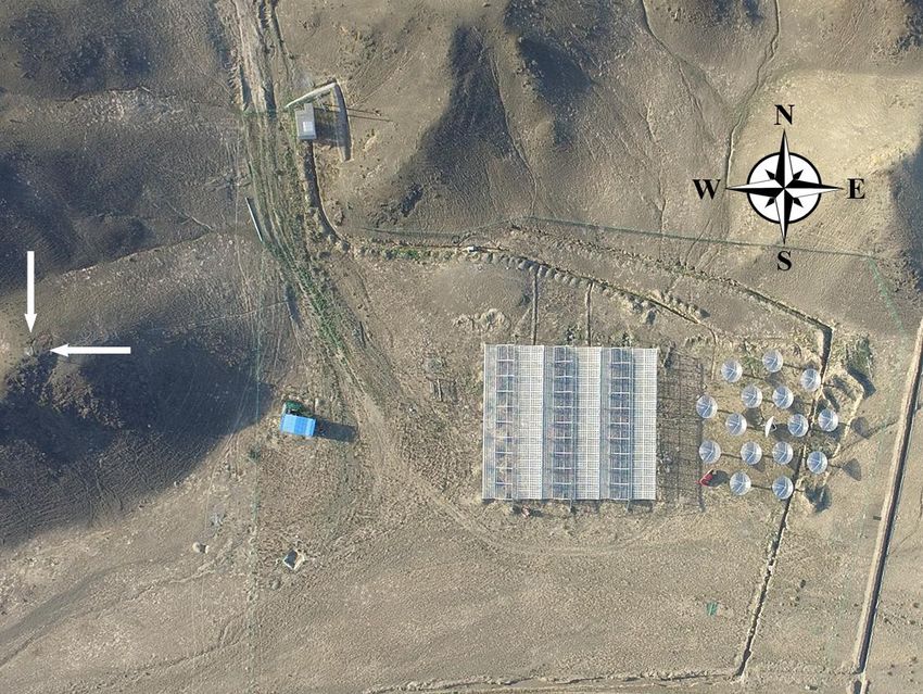
2     Fengquan Wu et al.
interferometer and is co-located with the Tianlai Cylinder         compact arrangement in order to provide sensitivity at the
Pathfinder Array, an interferometric array of 3 cylinder reflec-   relatively large scales (0.5 & k & 0.05) where the BAO fea-
tors in Xinjiang, China (Das et al. 2018; Tianlai 2021). These     tures appear in the power spectrum.
complementary designs were chosen specifically for testing            Although the 21 cm intensity mapping approach has been
approaches to 21 cm intensity mapping. Both arrays saw first       used for over a decade, it faces significant challenges. The
light in 2016.                                                     most significant is the fact that the 21 cm signal is roughly 4
   21 cm intensity mapping is a technique for measuring the        orders of magnitude dimmer than foreground emission (pri-
large scale structure of the universe using the redshifted         marily synchrotron radiation) from Galactic and extragalac-
21 cm line from neutral hydrogen gas (HI) (Liu & Shaw 2020;        tic radio sources. Analysis techniques for extracting the 21 cm
Morales & Wyithe 2010). It is an example of the general case       signal generally rely on the fact that foreground emission is
of line intensity mapping (Kovetz et al. 2019), in which spec-     a slowly-varying function of frequency while the 21 cm spec-
tral lines from any species, such as CO and CII, are used to       trum has structure arising from the large-scale distribution of
make three-dimensional, “tomographic” maps of large cos-           matter along the line of sight (Liu & Shaw 2020). However,
mic volumes. 21 cm intensity mapping is used to study the          instrumental effects, such as the delay term, can introduce
formation of the first objects during the Cosmic Dawn and          structure into the spectrum of otherwise smooth foregrounds.
the Epoch of Reionization (6 . z . 50) and for addressing          In particular, the spatial angular dependence of the antenna
other cosmological questions with observations in the post-        patterns is also frequency dependent and, in a process called
reionization epoch (z . 6), such as constraining inflation         ‘mode-mixing,’ couples the angular dependence of the bright
models (Xu et al. 2016) and the equation of state of dark          foregrounds into frequency dependence that masquerades as
energy (Xu et al. 2015). In the latter epoch, the approach         cosmic 21 cm structure. In addition, although the 21 cm sig-
provides an attractive alternative to galaxy redshift surveys.     nal is unpolarized, the bright foregrounds are partially po-
It measures the collective emission from many haloes simulta-      larized, and frequency-dependent instrumental ‘leakage’ of
neously, both bright and faint, rather than cataloging just the    Stokes Q, U, and V into I introduces another type of fore-
brightest objects. As a result, the required angular resolution    ground with a complicated spectrum. Faraday rotation in the
is relaxed as individual galaxies do not need to be resolved.      interstellar medium creates further spectral structure in the
By observing with wide-band receivers one simultaneously           polarization signal. Removing mode-mixing effects requires
obtains signals over a range of redshifts and can construct a      detailed understanding and measurement of the frequency-
tomographic map. The primary analysis tool for cosmologi-          dependent gain patterns of the antennas and of the gain and
cal measurements is the three-dimensional power spectrum of        phase of the instrument’s electronic response: i.e. calibration.
the underlying dark matter, and intensity mapping provides         To determine the scale of the calibration challenge, (Shaw
a natural means to compute this spectrum over a range of           et al. 2015) performed detailed simulations of the CHIME
wave numbers, k, in which the perturbations are in the lin-        interferometer’s ability to measure the HI signal in the pres-
ear regime. Of particular interest in the power spectrum are       ence of foregrounds. They showed it is necessary to know the
the baryon acoustic oscillation (BAO) features, which can be       beamwidth of the antennas to 0.1% and the electronic gain to
used as a cosmic ruler for studying the expansion rate of the      1% within each minute of observation to recover the unbiased
universe as a function of redshift.                                power spectrum of the HI signal.
   So far, the 21 cm signal has been detected with inten-
                                                                     Unlike most radio interferometers, all currently operating
sity mapping by two instruments: the Green Bank Telescope
                                                                   or proposed post-EoR HI intensity mapping instruments ob-
(GBT) (Masui et al. 2013; Switzer et al. 2013) and the Parkes
                                                                   serve by drift scanning the sky. This observing strategy allows
Observatory (Anderson et al. 2018) by cross-correlating in-
                                                                   for large sky coverage using simple and inexpensive instru-
tensity maps with galaxy redshift surveys.
                                                                   ment designs but requires new types of calibration strategies.
   While HI intensity mapping is being used out to a redshift      Tracking instruments can calibrate continuously on bright
of ∼ 50 to study the EoR and Cosmic Dawn by a variety              sources in, or near, the field they are mapping. Drift scan-
of instruments, including LOFAR (van Haarlem et al. 2013),         ning instruments like Tianlai must wait for bright sources to
MWA (Tingay et al. 2013), HERA (DeBoer et al. 2017), PA-
                                                                   pass through the field, or attempt to calibrate on dimmer
PER (Parsons et al. 2010), and LWA (Eastwood et al. 2018),         sources. Therefore, much of the discussion in this paper fo-
this paper focuses on measurements of the post-reionization        cuses on measuring the instrument stability and performing
epoch. Several dedicated instruments have been constructed,        the calibration of the Tianlai Dish Array.
or are under development, to detect the 21 cm signal from
this epoch using intensity mapping, ultimately without the            Future intensity mapping interferometers may include
need for cross-correlation with other surveys: Tianlai (Chen       thousands of antennas (Cosmic Visions 21 cm Collaboration
2012; Das et al. 2018; Li et al. 2020, 2021), CHIME (Ban-          et al. 2018; Slosar et al. 2019) in order to increase sensitivity.
dura et al. 2014), HIRAX (Newburgh et al. 2016), BINGO             The only currently feasible way to correlate this many signals
(Battye et al. 2016) and OWFA (Chatterjee & Bharadwaj              is by using fast Fourier transform algorithms (i.e. an ‘FFT
2018). Other instruments being designed and built to test the      correlator’) that require that the antenna patterns from the
technique include BMX (Castorina et al. 2020) and PAON-4           dishes be identical. Anticipating the need for such advances,
(Zhang et al. 2016b; Ansari et al. 2020). These 21 cm instru-      this paper also characterizes the uniformity of the antenna
ments have several features in common: with the exception          patterns in the Tianlai Dish Array.
of BINGO, they are all interferometers, achieving modest an-         This paper uses a small fraction (a few hundred hours)
gular resolution at modest cost; they have large numbers of        of the data collected to date in order to quantify basic per-
receivers in order to provide enough mapping speed to de-          formance characteristics of the Tianlai Dish Array. Future
tect the faint 21 cm signal; and the arrays are laid out in a      analysis of this data set will focus on making and cleaning

MNRAS 000, 000–000 (2020)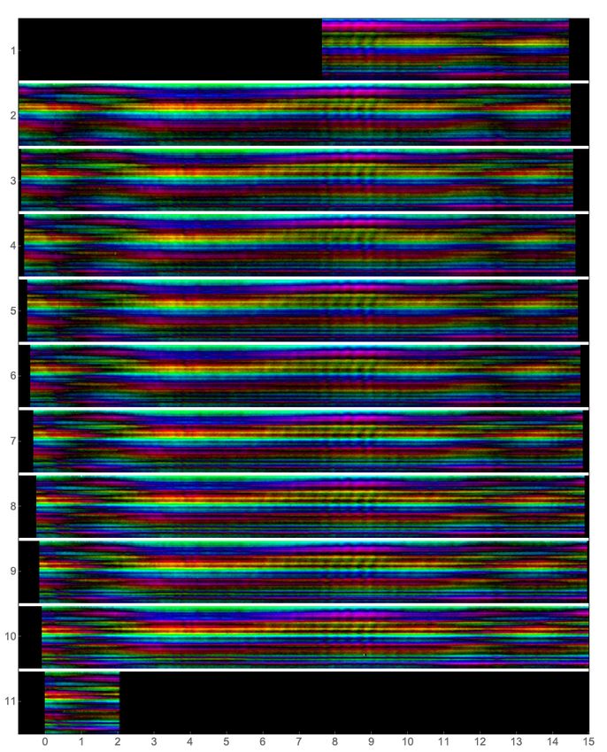
Tianlai Dish Pathfinder Array                3
maps of the NCP region, for which we have 3,700 hours of           ically. The motors can steer the dishes to any direction in
observations.                                                      the sky above the horizon. The drivers are not specially de-
   This paper is organized as follows: Section 2 describes the     signed for tracking celestial targets with high precision. In-
Tianlai Dish Array; Section 3 describes the observations car-      stead, in the normal observation mode, we point the dishes
ried out by the Tianlai Dish Array from 2016–2019; Sec-            at a fixed direction and perform drift scan observations. The
tion 4 compares the measured antenna patterns with simu-           Alt-Azimuth drive provides flexibility during commissioning
lations and evaluates their uniformity; Section 5 provides an      for testing and calibration. The dish array was fabricated by
overview of the data analysis process; Section 6 describes the     CASIC-23.1
gain and phase calibration process and Section 6.5 presents           The dishes are currently arranged in a circular cluster (Fig-
the results of this calibration in terms of noise level, and       ure 1). The array is roughly close-packed, with center-to-
sensitivity vs. integration time; Section 7 presents maps of       center spacings between neighboring dishes of about 8.8 m.
bright calibration sources; Data from several constant dec-        The spacing is chosen to allow the dishes to point down to el-
lination scans, corresponding to a total observation time of       evation angles as low as 35◦ without ‘shadowing’ each other.
more than 100 hours, have been used for the analysis pre-          One antenna is positioned at the center and the remaining
sented in sections 6 and 7. Section 8 describes results of long    15 antennas are arranged in two concentric circles around
integrations on the North Celestial Pole (NCP), using data         it. It is well known that the baselines of circular array con-
from 10 nights of January, 2018, conclusions and plans for         figurations are quite independent and have wide coverage of
the future appear in Section 9.                                    the (u, v) plane. A comparison of the different configurations
                                                                   considered for the Tianlai Dish Array and the performance
                                                                   of the adopted configuration can be found in Zhang et al.
                                                                   (2016b). The Tianlai dishes are lightweight and the mounts
2 INSTRUMENT                                                       are detachable, so, in future, the dishes can be moved to new
The objective of the Tianlai program is to make a 21 cm in-        configurations if required. This paper describes observations
tensity mapping survey of the northern sky. At present the         with the current configuration.
Tianlai program is in its Pathfinder stage, which aims to test        A schematic of the RF analog system can be found in Fig-
the technology for making 21 cm intensity mapping observa-         ure 2. The whole system except filters has been designed to
tions with an interferometer array. The Pathfinder comprises       operate over a wide range of frequencies (400–1500 MHz).
two arrays, one consisting of dish antennas and the other of       The low noise amplifiers (LNAs) are designed to have low
cylinder reflector antennas, both located at a radio quiet site    noise temperature (about 47 K at room temperature (Li et al.
(44◦ 90 N, 91◦ 480 E) in Hongliuxia, Balikun County, Xinjiang      2020)) and are mounted to the back of the feed antennas. The
Autonomous Region, in northwest China. In order to avoid           amplified RF signals pass through 15-meter long coaxial ca-
radio-frequency interference (RFI) generated by the correla-       bles to optical transmitters mounted under the dish antennas.
tor, the station house, which includes an analog electronics       The RF signal amplitudes modulate optical transmitters so
room, a digital correlator room (shielded from the analog          that the RF signals are converted to optical signals, which are
room), and living quarters, is located 5.8 km (11.2 km by          then transmitted to the station house via 8 km optical fiber.
road) away from the telescope site. A power line and optical       At the RF analog system room in the station house, the opti-
fiber cables about 8 km long connect the correlator building       cal signal is converted back to the RF electric signal. Replace-
with the antenna array. Construction of the Pathfinder ar-         able bandpass filters with 100 MHz bandwidth are mounted
rays was completed in 2016 and they are now taking data on         between the optical receivers and analog downconverters. An
a regular basis. This paper focuses on the dish array. Fur-        analog mixer then downconverts the RF signal to the 135–235
ther details about the cylinder array appear in Zhang et al.       MHz intermediate frequency (IF) band. Finally, the IF signal
(2016a); Cianciara et al. (2017); Das et al. (2018); Zuo et al.    is sent to the digital system through bulkhead connectors be-
(2019); Li et al. (2020, 2021).                                    tween the analog and digital rooms. The dishes currently ob-
   For each array, the feed antennas, amplifiers, and reflectors   serve in the frequency band 700–800 MHz (1.03 > z > 0.78)
are designed to operate from 400 MHz to 1430 MHz, corre-           in 512 frequency channels (δν = 244.14 kHz, δz = 0.0002).
sponding to 2.55 ≥ z ≥ −0.01. The instrument can be tuned             The digital backend system of the dish array is a 32-input
to operate in an RF bandwidth of 100 MHz, centered at any          correlator that consists of three FPGA boards: two process-
frequency in this range by adjusting the local oscillator fre-     ing boards for signal sampling and processing, and one for
quency in the receivers and replacing the band pass filters.       control. The Analog to Digital Converters (ADC) in the pro-
Currently, the Pathfinder operates at 700 − 800 MHz, corre-        cessing boards convert the RF signal to time series data at a
sponding to HI at 1.03 ≥ z ≥ 0.78. Future observations are         sampling rate of 250 MSPS and sampling length of 14 bits.
planned in the 1330 − 1430 MHz band (0.07 ≥ z ≥ −0.01) to          Then the FPGA chips in the processing boards perform the
facilitate cross correlation with low-z galaxy redshift surveys    FFT of the time series data. The two FPGA boards exchange
and other low-z HI surveys.                                        half of the signal channels with each other through rapidIO
   The Tianlai Dish Array consists of 16 on-axis dishes.           cables, so all cross-correlations are computed in the FPGA
Each has an aperture of 6 m. The design parameters of the          boards while the computation loads on the boards are bal-
dishes are shown in Table 1. The dishes are equipped with          anced. Finally, the visibility from the dish array (32 auto-
dual, linear-polarization receivers, and are mounted on Alt-       correlations and 496 cross-correlations) are sent to a storage
Azimuth mounts. One polarization axis is oriented parallel
to the altitude axis (horizontal, H, parallel to the ground))
and the other is orthogonal to that axis (vertical, V) Zhang
et al. (2020). Motors are used to control the dishes electron-     1   http://www.casic23.com.cn

                                                                                                      MNRAS 000, 000–000 (2020)
4     Fengquan Wu et al.

Figure 1. Left: Top view of the Tianlai Dish Array Pathfinder and Cylinder Array Pathfinder taken with a DJI M600 Pro drone at a
height of 280 m above the ground. The position of the calibration CNS is indicated by the white arrows on the left. The relative distance
vector from the feed in dish 16 at the center of the array (when pointed toward the zenith) to the CNS is [-184.656, 13.915, 12.588] meters,
with x,y,z to the east, north, and zenith. The CNS is in the far-field of all dishes in the dish array. Right: A schematic diagram of the
Tianlai Dish Array; 0◦ coincides with North.
    The dishes are arranged in two concentric circles of radius 8.8 m and 17.6 m around a central dish. The dishes have dual-linear
  polarization feed antennas with one axis oriented parallel to the altitude axis (horizontal, H, parallel to the ground)) and the other
    orthogonal to that axis (vertical, V). For example, shown in red is one of the baselines that is studied later in this paper, the H
polarization of dish 4 correlated with the H polarization of dish 9: 4H-9H. Other baselines used later in the paper use the same naming
                                                               convention.

                                             Figure 2. Schematic of the RF analog system.

Table 1. Main design parameters of a Tianlai dish antenna.              be performed using bright astronomical standard calibration
                                                                        sources. However, for small aperture arrays like the Tianlai
    Reflector diameter            6m                                    Dish Array, there are not enough bright sources on the sky
    Antenna mount                 Alt-Az pedestal                       to meet the requirement of point source calibration, so we
    f/D                           0.37                                  have designed a dedicated calibration noise source (CNS) to
    Feed illumination angle       68◦                                   provide relative calibration. A broadband RF noise generator
    Surface roughness (design)    λ/50 at 21 cm                         is placed in a thermostatically controlled environment and is
    Altitude angle                8◦ to 88.5◦                           supplied with regulated DC power to ensure the stability of
    Azimuth angle                 ±360◦                                 the RF amplitude. The on-off timing of the CNS is controlled
    Rotation speed of Az axis     0.002◦ ∼ 1◦ /s
                                                                        by a clock signal carried by optical fiber from the correlator
    Rotation speed of Alt axis    0.002◦ ∼ 0.5◦ /s
                                                                        8 km away in the station house.
    Acceleration                  1◦ /s2
    Gain(design)                  29.4+20log(f/700 MHz) dBi
    Total mass                    800 kg
                                                                        3 OBSERVATIONS
                                                                        As of the end of 2019, we had collected about 6, 200 hours
server by two ethernet cables and dumped to hard drives in              of observational data from the Tianlai Dish Array, including
HDF5 format.                                                            more than 5700 hours of NCP data. In Figure 3 we show
   Calibration of the electronic gain of the receivers is cru-          the accumulated observing time over the years. Details of
cial for any interferometer, and it is especially important for         individual runs are listed in Table 2. Drift scans are per-
Tianlai to compensate for phase variation in the 8 km long              formed at constant declination over several days at a time.
optical cables. The absolute calibration of the system can              These can be divide into two types: (1)24 hr observations

MNRAS 000, 000–000 (2020)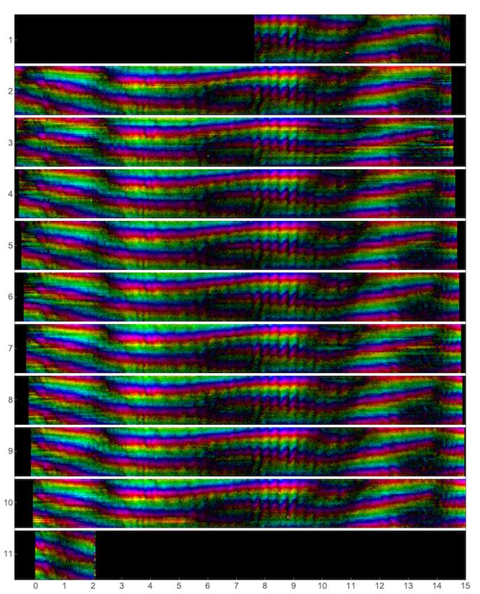
Tianlai Dish Pathfinder Array 5
Table 2. Observation log for the Tianlai Dish Array from 2016 to late 2019.
Data Set Date Calibration Sources Targets Length (hours)
Data 201605-06 May 2016 None Cygnus A 72
CygnusANP 20170812 Aug 2017 Cygnus A North Pole 67
CasAs 20171017 Oct 2017 None North Pole 147
CasAs 20171026 Oct 2017 None Cassiopeia A 290
3srcNP 20180101 Jan 2018 3C48, Cassiopeia A, M1 North Pole 241
2srcNP 20180112 Jan 2018 3C48, M1 North Pole 97
IC443NP 20180323 Mar 2018 IC443 North Pole 181
M87NP 20180407 Apr 2018 M87 North Pole 90
2srcNP 20180416 Apr 2018 IC443, M87 North Pole 142
3srcNP 20181212 Dec 2018 Cassiopeia A, 3C48, M1 North Pole 757
1DaySun 20190113 Jan 2019 None Sun 48
3srcNP 20190128 Jan 2019 Cassiopeia A, 3C48, M1 North Pole 741
3srcNP 20190228 Feb 2019 3C123, M1, IC443 North Pole 764
3srcNP 20190402 Apr 2019 M1, IC443, 3C273 North Pole 522
3srcNP 20190611 Jun 2019 M87, Hercules A, Cygnus A North Pole 737
3srcNP 20190830 Aug 2019 3C400, Cygnus A, Cassiopeia A North Pole 924
3srcNP 20191022 Oct 2019 3C400, Cygnus A, Cassiopeia A North Pole 302
Figure 3. Accumulated observing time vs. date.
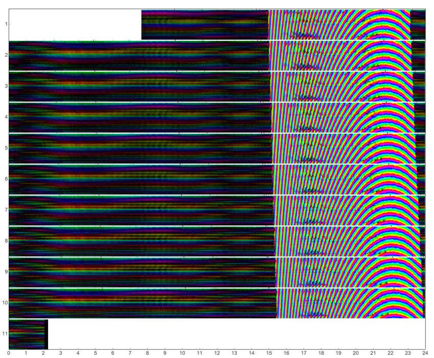
Figure 4. Masking of the CNS and RFI after applying both the
sum threshold method and the SIR operator method. The vertical
lines show times and frequencies masked when the signals from
the CNS are used for calibration. Apart from the CNS we can
at declinations away from the NCP, usually at the declina- see a very small amount of data at discrete frequencies and times
tion of bright sources: Cyg A (+40◦ 440 ), Cas A (+58◦ 48.90 ), masked as RFI. Because the amount of RFI is very small we have
Tau A/M-1 (+22◦ 000 ) and also some high declination regions blown up a bandwidth of about 50 MHz where some RFI is visible.
(∼ 80◦ ). (2) 24 hour observations at the NCP. Preceding each Some faint horizontal lines (at about 777 MHz and 767 MHz) are
NCP observation, the antennas are pointed towards one or from intermittent RFI.
multiple strong radio sources for calibration. The calibration
sources for different NCP observations are listed in Table 2.
The visibilities from the dish array are averaged for a pe- reduced to 4 s per 4 min, which is 1.67% of the observing
riod of 1 s (integration time). The data are stored for all time.
528 correlation pairs (auto-correlation + cross-correlation) In Figure 4 we show the CNS and RFI mask derived from
in 512 different frequency channels. The data rate is about 1 hour of nighttime data. The periodic vertical stripes show
∼ 175 GB/day. The weather data, which includes the tem- the mask when the CNS is turned on, while the dots show
perature of the analog electronics room, site temperature, the RFI. We use two different RFI cleaning methods (check
dew point, humidity, precipitation level, wind direction, wind Sec. 5). Because the array is located in a radio quiet zone, we
speed, barometric pressure, etc., are stored separately during only lose about 0.6% of data due to RFI contamination.
each run. These data can later be used for checking the cor-
relation of different weather variables with the variation of
electronic gain of the system.
4 BEAM PATTERNS
The CNS is turned on and off periodically. During 2017
the CNS switched on for 20 s every 4 min, so the fraction Separating the faint 21 cm signal from strong foregrounds re-
of noise-on time is ∼ 8.33%. In 2018, the noise-on time was quires exquisite knowledge of the frequency-dependent beam
MNRAS 000, 000–000 (2020)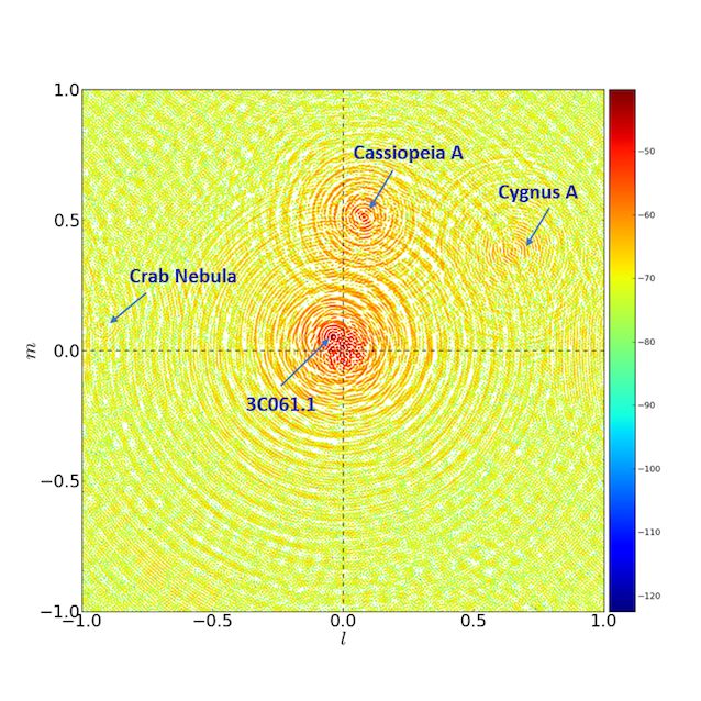
6     Fengquan Wu et al.

Figure 5. Measurements and simulations of the H-plane antenna pattern of the V-polarization of one dish. Left: Pattern measured with
the UAV compared with two electromagnetic simulations. Right: Patterns measured both by an UAV and by a transit of Cas A. In both
figures the UAV flies in the E-W direction and the measurements and simulations are performed at 730 MHz.

patterns of the antennas. Small imperfections in the anten-         ments and simulations appears in Zhang et al. (2020). An
nas or changes in the environment (e.g., temperature, wind)         UAV outfitted with a broadband noise source is flown in the
can affect the beam patterns and introduce systematic errors        far field along two paths over antenna # 6, at the edge of
in the measurement. In addition, future arrays with large           the array: a north-south path and an east-west path. The
numbers of antennas will likely require highly uniform anten-       E- and H-plane patterns are measured for each flight path
nas to exploit techniques such as redundant calibration and         over the 700-800 MHz band. As an example, Figure 5 shows
FFT correlation (Tegmark & Zaldarriaga 2009; Tegmark &              the H-plane measurement for the east-west path at 730 MHz.
Zaldarriaga 2010; Sievers 2017; Byrne et al. 2020). However,        Multiple flights are conducted at different RF power levels to
to our knowledge, detailed requirements for the precision of        map the beam into the far sidelobes. Figure 5 (Right) shows
knowledge of beam patterns and sidelobes and cross-polar            the beam pattern measured by the UAV and compares it with
response, their stability with time, their required degree of       the profile of the main beam measured at the same frequency
uniformity, and relative pointing accuracy have not yet been        using the auto-correlation signal from one polarization dur-
performed. Nevertheless, Shaw et al. Shaw et al. (2015) pro-        ing a transit of Cas A. The Cas A signal is not bright enough
vide a relevant data point, showing that to control foreground      to measure the sidelobes of the antenna.
contamination from mode-mixing, the dish beamwidths must               We also performed electromagnetic simulations of the feed
be known and uniform to 0.1%.                                       antenna and the dish reflector using commercially-available
   We have taken preliminary steps toward characterizing the        software.2 We overplot the simulated beam pattern with the
beam patterns using transits of bright radio sources and scans      UAV measurement in Figure 5 (Left). The patterns match
with a radio source flown over the array on an unmanned             well in the main lobe and the measured position and width
aerial vehicle (UAV). We find reasonable agreement between          of each sidelobe shows good agreement with the simulation.
the beam measurements and the electromagnetic models. The           However, the UAV measurements show a “shoulder" at ±6◦ ,
dirty maps of bright sources shown in Section 7 do not re-          an asymmetry in the sidelobes, and a stronger signal in the
quire knowledge of the beams, however, the temperature cal-         sidelobes.
ibration described in Section 6.3, which is used for the anal-         We compare these measurements of the antenna
ysis of 10 nights of integration on the NCP in Section 8,           beamwidths and sidelobes to electromagnetic simulations of
requires measuring the response of the instrument to astro-         the effects of errors in shapes of the dishes. We have not yet
nomical calibration sources as well as knowledge of the direc-      performed measurements of the dish shapes (e.g. with pho-
tivity gain of the antennas. The latter requires knowing the        togrammetry), so rely on simulations of random errors in the
beam pattern in all directions. Because we have not yet mea-        reflector surface. We consider random errors on both large
sured the beam patterns into the far sidelobes, for now we          scales and small scales. For large-scale errors (on the scale of
rely on the simulations for determining the directivity gain.       10’s of cm), simulations were performed using two simulation
Rough agreement between measurements and simulations in             packages, CST and FEKO. Errors were simulated with am-
the main beam is encouraging, but extending measurements            plitudes as large as 30 mm, 7 times larger than the surface
over the full beam remains an important research goal. Fu-          roughness specification for the dish (0.02λ at λ = 21 cm),
ture deconvolved maps of the NCP will require knowledge of          which was built with standard antenna construction tech-
the main beam.                                                      niques. These simulations widen the FWHM of the beam by
                                                                    less than 0.2◦ and increase the level of sidelobes by less than
   Furthermore, as is the case for other interferometers de-
                                                                    6 dB. We used similar simulations to investigate the effect of
signed for HI intensity mapping, the primary beam patterns
                                                                    errors in the placement of the feed antennas. Simulated dis-
of the Tianlai dish antennas are affected by the presence of
                                                                    placements of the feed antenna from the nominal focus by as
the other antennas in the array. Both the UAV measurements
                                                                    much as +50 mm (away from the dish) and -10 mm (toward
and the electromagnetic simulations show an asymmetry in
                                                                    the dish) can increase the FWHM of the dishes by about the
the beam patterns and an increase in the sidelobe levels com-
pared to simulations of isolated antennas. This phenomenon
has implications for the design of future HI arrays.                2 CST Studio Suite https://www.3ds.com/products-services/
  Figs. 5 and 6 summarize the antenna beam measurements             simulia/products/cst-studio-suite/ and FEKO https://www.
and simulations. A detailed description of the UAV measure-         altair.com/feko/

MNRAS 000, 000–000 (2020)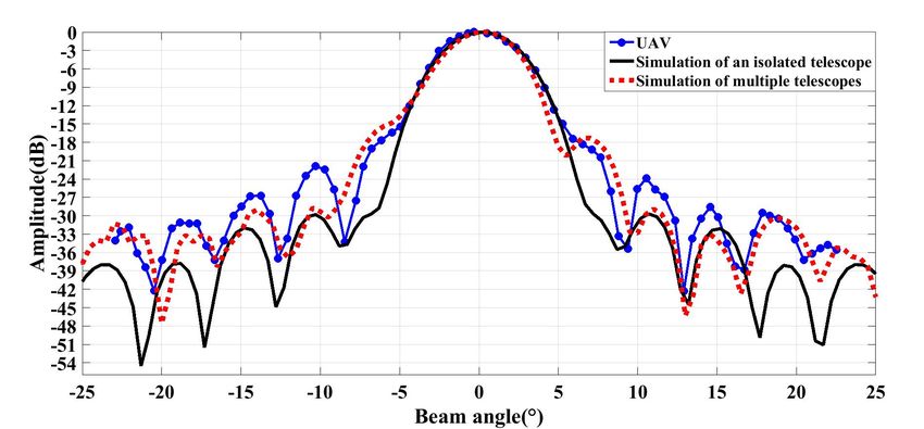
Tianlai Dish Pathfinder Array                   7

Figure 6. Simulated beam patterns as a function of beam angle
θ from the beam center of the antennas for 3 different frequencies,
700 (red), 750 (green) and 800 MHz (blue). Each plot shows the
absolute co-polar directive gain in dBi, averaged over the azimuthal
angle. Angle θ is the polar angle, calculated from the center of
the beam. The simulations show that the antenna sidelobes vary
significantly as a function of frequency.

amount we measure with the UAV, but this displacement
is larger than the tolerance on the placement of the feed.
These focus displacements have no significant effect on the
sidelobes. For small-scale errors, we estimate the effects of
random surface deviations of λ/50 at 21 cm, the design spec-
ification given for surface roughness of the dishes. Using an-         Figure 7. Plot of the mean FWHM of the main beam vs. frequency
tenna tolerance formulasRuze (1966); Rahmat-Samii (1983),              using daily transits of Cas A over 12 days. The measurement is for
we estimate the FWHM would increase less than 3% and the               a fairly typical baseline. The top figure represents the horizontal
sidelobe peak values would increase by less than 1 dB. Hence,          baseline (4H-9H), which primarily measures the E-plane of the
neither large-scale or small-scale errors in the dish surface or       antenna, while the lower figure represent the vertical baseline (4V-
focus are consistent with the measurements of the main beam            9V), primarily measuring the H-plane. The black line shows the
                                                                       mean in each frequency bin over this period and the red scatter plot
or sidelobes obtained with the UAV (Figure 5).
                                                                       shows the FWHM for each day. The frequency binning is 244 kHz.
   A simulation that shows the same beam asymmetry and
                                                                       The green line shows the expected FWHM vs. frequency based on
similar sidelobe levels as the UAV measurement includes dish           an electromagnetic simulation. For reference, the blue line shows
# 6 as well as 4 adjacent dishes in the array (dish #5, #7,            the FWHM of a uniformly-illuminated Airy disk with an effective
#13, and #14). It is shown as the dashed red line in Figure 5.         diameter Deff that is 90% of the actual 6 meter diameter.
We conclude that these effects arise, at least partially, from
scattering from other dishes in the array. Scattering from the
ground and nearby hills is not included in the current sim-            beam in the E- and H-planes is also calculated by the elec-
ulations. Simulating the full array and the ground requires            tromagnetic simulations; the simulated FWHM is co-plotted
more computing resources that we currently have available.             for comparison. We also plot the case of a diffraction - lim-
Ultimately, we plan to extend these simulations and measure-           ited circular aperture (1.028λ/Deff with Deff = 0.9D). (The
ments to all the dishes in the array, plus the ground, over the        1.028 prefactor comes from the FWHM of an Airy pattern
full range of frequencies. Simulations extended into the far           from a uniformly illuminated disk.) The measured and sim-
sidelobes and backlobes of an isolated antenna are shown in            ulated beamwidths differ by about 0.3 − 0.5 degrees. This
Figure 6.                                                              discrepancy originates in a corresponding difference between
   As mentioned in Section 1, knowledge of the beam patterns           the measured and simulated beams of the feed antennas. The
of each antenna as a function of frequency, and the stability          broad ripples in the frequency-dependence of the beamwidth
of the pattern with time, are also important factors. Figure 7         in Figure 7 are consistent with the appearance of standing
shows the FWHM of one cut through the beam pattern from                waves between the feed antenna and the dish surface. The
a pair of antennas as a function of frequency. The pattern             path length from the feed to the dish and back again is twice
is measured repeatedly in the E-W direction by observations            the 2.2 m focal length, and should introduce ripples with a
of the transit of Cas A on 12 successive days starting on              period of 68 MHz, close to the observed period. Ripples with
2017/10/26. For each transit, the magnitude of one visibil-            similar amplitudes and periods appear in both the measure-
ity vs. time is fit to a Gaussian. The measured pattern is             ments and the simulations, but the phases of these do not
effectively the geometric mean of the patterns of two dishes,          line up in the V baseline as well as they do in the H baseline.
which are nominally coaligned. Day-to-day fluctuations of the          We are trying to understand the reason for this discrepancy.
FWHM are less than 1%. The frequency dependence of the                 Another known reflection in the system occurs at the ends

                                                                                                            MNRAS 000, 000–000 (2020)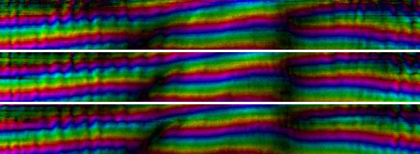
8     Fengquan Wu et al.

Figure 8. The black line shows the mean FWHM vs. frequency for
118 H-H baselines during a transit of M1 on 2018/01/02. The plot
excludes auto-correlations, baselines with known faulty probes,
and other outliers.                                                 Figure 9. Variations of the modulus of the cross-correlation vis-
                                                                    ibilities between the Tianlai dishes with time (in seconds) during
                                                                    a transit of Cas A. Each of the 120 cross-correlations corresponds
                                                                    to one color. The black curve shows the expected response from
                                                                    a simplified simulation (from a 5.4 m diameter dish with a Gaus-
of the 15 m coaxial cable between the feeds and the optical         sian beam). All (un-calibrated) cross-correlations have been renor-
transmitter (Figure 2). Ripples caused by this reflection cor-      malized to unity at their respective maxima. The observed time
respond to a period of 7 MHz, which is barely visible in the        spread between the cross-correlations reflects the dishes’ relative
top plot of Figure 7, in addition to the dominant 68 MHz            E-W pointing dispersion. The green dip at around 6000 s is an
ripple.                                                             artifact from the CNS interpolation. Each curve is the average of
   Another important characteristic of the antenna patterns         40 frequency channels (742.6172 MHz to 752.1387 MHz, with each
is the uniformity of the different antennas. Here we estimate       frequency bin being 244 kHz), near the center of the RF band.
the uniformity of the beamwidths of the dishes in the Tianlai
Dish Array by using transit observations of M1 to determine
the effective beamwidth of all pairs of antennas (baselines).
Figure 8 shows the mean value of the FWHM of 118 baselines
in the array and the 1-sigma deviations from the mean as a
function of frequency. The 1 − σ deviations are ∼ 4%.
   We have also studied the pointing accuracy of the dishes
in the E-W direction. Using data from the Cas A transit
of 2017/10/30, we compare in Figure 9 the variations of the
modulus of the visibilities formed by the cross-correlation be-
tween the dish signals. (In cross-correlation the Cas A signal
is almost undistorted by the diffuse Galactic signal; this is
not the case for auto-correlations, which are affected by the
diffuse background.) To get a rough measurement of the E-W
pointing accuracy, we have extracted the peak position from
each of these cross-correlations by fitting a Gaussian curve.
If the times of the peak response for two dishes are t1 and t2 ,
the peak time of the cross-correlation will be their average
peak time, t12 = (t1 + t2 )/2, so the variance σ 2 for the cross-
                                                                    Figure 10. Extracted transit time differences w.r.t. to the expec-
correlation is only half of that for a single dish. The point-
                                                                    tation from a simplified simulation, for the 16 Tianlai dishes from
ing of the antennas in the E-W direction can be regarded as         the Cas A transit of 2017/10/30. The ∼ 150s FWHM of these time
a Gaussian distribution centered on the expected
                                              √         pointing.   shifts from cross-correlation corresponds to an E-W pointing error
If the σ 2 is doubled, the FWHM will be 2 times larger,             of ∼ 0.47 degrees on the sky (not in RA). This indicates an E-W
because FWHM ∝ σ. As illustrated in Figure 10, the E-W              pointing error of ∼ 0.66 degrees for a single dish.
pointing spread from cross-correlation indicates a 0.47 degree
FWHM dispersion (on the sky), so the E-W pointing disper-
sion of single dish will be about 0.66 degree. This dispersion      about 0.05 − 0.2◦ , so loading by the wind on the reflectors
is roughly consistent with our current procedure for aligning       will introduce an additional pointing uncertainty.
the pointing of the dishes. We calibrate the absolute pointing         Pointing accuracy in the N-S direction is difficult to deter-
of each dish by observing the shadow of the Sun projected           mine using transits of astronomical sources, as is dependence
onto the vertex of the parabolic reflector surface when the         of the beam shape on elevation angle. (Elevation changes will
dishes are pointed at the Sun. We estimate this process can         introduce mechanical deflection of the dishes.) Currently, our
introduce pointing errors of about 0.2◦ . In addition, back-        absolute calibration procedure requires pointing the dishes
lash in the antenna gears introduces an additional error of         toward radio sources at different elevation angles than our

MNRAS 000, 000–000 (2020)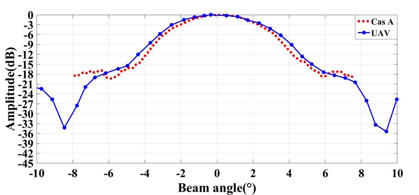
Tianlai Dish Pathfinder Array                  9
primary science target, the NCP. In principle, full 2π beam           The overall data processing workflow of tlpipe appears
patterns could be measured using the UAV Chang et al.               in Figure 12. The list of tasks is entered into a *.pipe file.
(2015); Jacobs et al. (2017) to determine changes in the beam       The task manager takes the file as an input and applies the
shapes and pointing accuracy as well as the far-sidelobe pat-       tasks to the data container in sequence. The tasks, in gen-
terns. The UAV measurements described here concentrated             eral, modify the visibility and the mask array in the data
on characterizing a single dish, but, given the relatively small    container.
size of the Tianlai arrays, we plan future measurements to
map all the dishes in the array simultaneously when pointed
at the NCP and at the elevation angles of calibration sources.      5.2 Built-in data processing tasks
   Using the UAV, we have placed an upper limit on the cross-
                                                                    In the tlpipe package, we have implemented more than 30
polar response of antenna #6. At the center of the beam, the
                                                                    tasks. Users can write their own independent tasks to apply
cross-polar response is less than about 1% across the band.
                                                                    to the data container. Some of the built-in tasks in the tlpipe
(See Zhang et al. (2020) for details of the measurement.)
                                                                    are as follows:
This is consistent with simulations, which predict about 0.4%
cross-polar response across the band.
                                                                    Masking of the CNS The Tianlai data contain periodic
                                                                    calibration signals from the CNS which must me removed
                                                                    during analysis. A dedicated subroutine detects the pres-
5 OVERVIEW OF (OFFLINE) ANALYSIS                                    ence of the CNS signal by measuring the difference between
  PROCESS                                                           the amplitude of two consecutive data points in an auto-
For analyzing the Tianlai data we developed a Python                correlation channel and comparing it with the overall vari-
pipeline named tlpipe 3 . It is a collection of several stand-      ance. The routine calculates the turn-on and turn-off times
alone packages that can be used for reading the raw visibility      of the CNS and sets elements of a Boolean mask array to
data, masking, RFI flagging, calibration, data binning, map-        True when the CNS is on. In Figure 4 the masked CNS can
making, etc. Multiple visualization and other utility packages      be seen as periodic vertical straight lines.
have also been developed. The pipeline is written in a mod-
ular format and users can develop and add their own algo-           RFI cleaning After masking the CNS we need to clean RFI
rithms to the pipeline with little knowledge of how the rest        from the data. Multiple RFI flagging algorithms are available
of the pipeline works. Figure 11 shows the basic workflow           in tlpipe, but a combination of the sum threshold method
of the tlpipe for making maps from the raw visibility data.         (Offringa et al. 2010) and the scale-invariant rank (SIR) op-
A more detailed description appears in Zuo (2020). Tianlai          erator method (Offringa et al. 2012) work best for the Tianlai
and tlpipe use the HDF5 formats consistently. However, we           data. Visibility data points flagged as RFI are recorded in the
have successfully imported data from other interferometers          mask array. The RFI masked from 1 hour of nighttime data
saved in formats different from the HDF5 format defined for         using the sum threshold + SIR operator method is shown in
Tianlai, and then processed them with tlpipe.                       Figure 4.

                                                                    CNS calibration (relative calibration) Two methods for
5.1 tlpipe data processing workflow
                                                                    calibration are included in tlpipe. For absolute calibration
We use Python-2.7 as the main programming language. This            of the amplitude and phase of the gain we use strong as-
choice allows us to use its vast collection of scientific comput-   tronomical point sources (next section). However, as only a
ing libraries. However, some of the performance-critical parts      few bright sources are available and accessing them requires
have been compiled in C by using Cython. Parallel process-          repointing the dishes, we also perform relative calibrations
ing has been implemented with the Message Passing Interface         using a regularly broadcast CNS signal. The CNS calibration
(MPI) framework.                                                    is primarily used to remove the phase variations over time
  The basic workflow of tlpipe can be broken into 3 distinct        but we are studying its use for amplitude calibration as well.
components: task manager, tasks, and data container.                   We developed two different algorithms for the calibra-
                                                                    tion using the CNS. The first task, nscal, uses the CNS
Task manager: The task manager controls the overall flow            to calibrate each visibility. For each baseline, it defines the
of the pipeline and applies different Tasks to the data.            visibility during the on and off cycles of the CNS to be
                                                                      ON              NS        OFF
                                                                    Va,b   = Va,b + Va,b  and Va,b   = Va,b , where Va,b is the ob-
                                                                                                            NS
Tasks: Tasks are independent codes that operate on the data         served visibility from the sky and Va,b    is the visibility from
in the data container. These tasks include CNS removal, RFI         the CNS corresponding to the baseline a, b. The phase in-
                                                                                                                       ON       OFF
flagging, map making, and calibrations. We discuss some of          troduced by the CNS is then φa,b = Arg(Va,b            − Va,b   ).
the tasks in the next section.                                      Because the CNS phase is constant for a particular base-
                                                                    line, and the CNS amplitude is assumed to be constant, the
Data container: The data container holds the data oper-             corrected visibility from the sky, after the CNS calibration,
                                                                         NS−Cal                         NS
ated on by the pipeline. It includes an array of visibilities,      is Va,b      = exp(−iφa,b )Va,b /|Va,b |, where the CNS signal
a Boolean mask array corresponding to each visibility, and          is assumed to be much larger than the sky signal. In fact,
some supplementary data.                                            because the CNS signal enters through the sidelobes of the
                                                                    beam, its amplitude is not very stable. We use the CNS pri-
                                                                    marily for phase calibration. Further details appear in Zuo
3   https://github.com/TianlaiProject/tlpipe                        et al. (2019).

                                                                                                        MNRAS 000, 000–000 (2020)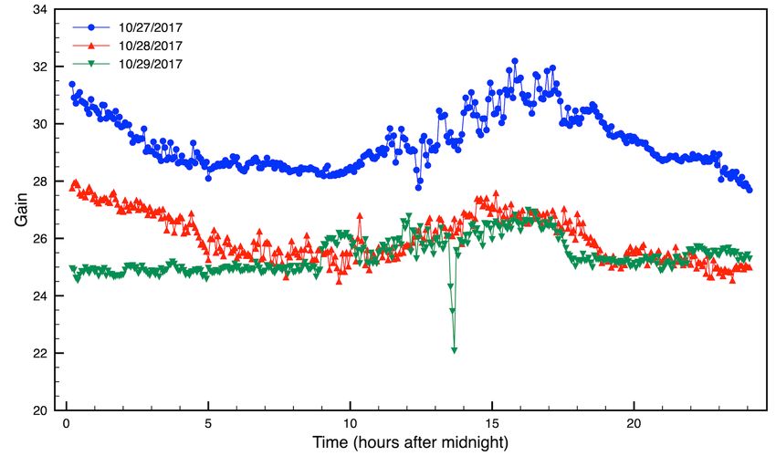
10      Fengquan Wu et al.

                                                                            Relative Phase                Amplitude and
                    Input Data                  RFI Flagging
                                                                             Calibration                 Phase Calibration

                                                  Sky Map                    map-making                    LST binning

                          Figure 11. Schematic of the data processing pipeline implemented in the tlpipe package

                                                                       See Zuo et al. (2019); Zuo (2020) for details. The computed
                                                Data container1
                                                                       gain is applied to the entire data set until the next point
                                 Task1                                 source transits.
                                                Data container2

     Task manager
                                                                       Map-making The built-in mapmaking code uses the
                                 Task2
                                                                       m−mode analysis from (Shaw et al. 2015, 2014; Zhang et al.
                                                Data container3        2016b). There are also independently-written mapmaking
                                 Task3                                 codes which we use for data analysis. Details are discussed in
                                                Data container4
                                                                       Sec. 7.

                                                                       Utility tasks and plotting tasks Apart from these stan-
Figure 12. This schematic describes the relation between               dard tasks, tlpipe includes multiple utility packages and
the three major components of the tlpipe data-processing
                                                                       plotting tasks. The utility packages include codes such as
pipeline.tlpipe implements two types of data container: the Raw-
                                                                       those for removing contamination by the Sun from the day-
Timestream and Timestream. The tasks take an instance of one of
the two data container types as input, and produce an instance of      time data. This technique uses an eigenvalue approach for re-
one of the two data container types as output. The input and out-      moving the largest eigenvalue from the daytime data and can
put can be the same instance (i.e. both RawTimestream or both          successfully remove 99% of the solar contamination. It will
Timestream), possibly with modified data and/or meta data, or          be described in a future publication. Other utility packages
different instances (i.e. input instance of RawTimestream, output      include removing bad channels, daytime masking, etc. The
instance of Timestream). Data are transferred from the input in-       plotting packages include codes for plotting waterfall plots,
stance to the output instance, then the input instance is destroyed.   plotting time or frequency slices of the data, etc.
The data container is the memory mapping of HDF5 files on disk.
Tasks operate on the data contained in the data container in mem-
ory. The data volume is not multiplied on disk.
                                                                       6 CALIBRATION

   The second task, nscalg, uses the CNS to perform a global           As described in Section 5, two complementary methods are
fit to the observed visibilites to determine an independent            used to calibrate the amplitude and phase of the electronic
(complex) gain for each feed. Because only phase differences           gains of the receivers. Transits of point sources are used to
between feeds matter, the phase of feed 1 is fixed to be               obtain absolute gain and phase calibrations, every few days,
zero without any loss of generality. The gain amplitudes re-           up to a maximum of two or three times per 24 hours, while
ported are relative to the (uncalibrated) CNS amplitude. This          the CNS calibration procedure allows tracking every few min-
method is used in the CNS calibration results shown in Sec. 6.         utes of the electronic phase calibration drift between the on-
Because the gain changes with time, a spline is fit to the mea-        sky bright source calibration. (In fact, for observations of the
sured gains and used to interpolate between CNS calibration            NCP region, where there are no bright point sources, point
events. Because there are only N gains but N ×N visibilities,          source calibration requires repointing the dishes away from
this process is not perfect.                                           the pole. In the future, calibration from bright point sources
                                                                       that appear in the antenna sidelobes (see Figure 22) may
Point source calibration (absolute calibration) After                  prove useful, but that topic is beyond the scope of this pa-
the relative phase calibration using the CNS, transits of              per.) In this section we apply these two types of calibration
strong astronomical radio sources are used to make an ab-              to the data and evaluate the stability of the array’s gain (am-
solute gain calibration that gives the actual amplitudes and           plitude and phase) over time.
phases of the complex gains for each feed. The solution is ob-
tained by fitting the transit signal for each of the N (N − 1)/2
                                                                       6.1 Gain stability measured with the CNS
visibilities (assuming known geometry) for each frequency, in-
dependently. The algorithm decomposes the 16 × 16 visibility           The response of the dishes to the CNS is not a smooth
matrix for each polarization to yield the complex gains for            function of frequency and the shapes of the response vary
the 16 feeds. The H and V feed gains are determined inde-              widely. Based on the comparison with astronomical point
pendently. Calibration is provided in units of K or Jy.                source calibration and normal observation data described in
   Again, there are two calibration routines. PSCal and                latter sections, we believe much of this frequency structure
PScal2 both use the same robust principal value decomposi-             arises because, for most observing directions, the CNS is cou-
tion to determine the gain of each feed, but have some differ-         pled to the antennas through their far sidelobes. Electromag-
ences in the handling of outliers and diagnostic information.          netic simulations of these far sidelobes demonstrate signifi-

MNRAS 000, 000–000 (2020)
Tianlai Dish Pathfinder Array 11
Figure 13. Left: Gain versus frequency for the cross-correlation of feeds 1H and 3H, measured using the CNS with nscalg. The amplitude
is in raw (uncalibrated) visibility units and the phase is in radians. Right: Gain versus frequency for the cross-correlation of feeds 3V and
16H. The amplitude is in raw (uncalibrated) visibility units and the phase is in radians. The two baselines used in this plot are fairly
typical.
cant variation with frequency and position of each dish with After applying nscalg, which determines the gains of the
respect to the CNS. For these reasons the CNS is used only individual feeds, we can test the calibration process by com-
to calibrate the relative phases of the gains of the receivers, puting the visibilities from the fitted feed gains and compar-
not their amplitudes. We are investigating whether it could ing them to the observations. Figure 15 shows such a test.
be used to calibrate the relative amplitudes as well. Figure The observed 1H-5H visibility (red data points, measured
13 (Left) is a “typical” H-H cross-correlation and Figure 13 when the CNS is on) is compared to the visibility that is
(Right) is a typical V-H cross-correlation. The plots show the expected using the fitted gains for feeds 1H and 5H. The
cross-correlation of feeds in different dishes, but when the visibility from the fitted gains can, of course, only be deter-
feeds are in the same dish the plots are similar. The phase mined when the CNS is active. However, we can connect the
plots have a phase and delay that is fit and subtracted from points when the CNS is active with a spline curve to pro-
the visibility phase so that the residual phase is close to zero. vide a calibration between the times when the CNS is active,
Note that the amplitude of the response of the H-H and V-H as shown by the blue curve in Fig 15. There is a small but
polarizations are similar. significant offset of about 0.04 radians, or about 2◦ , in the
Figure 14 shows the gain as a function of time for feed 5V phase, but the amplitude is well described by the curve. This
with respect to time for 3 consecutive days in October 2017. plot is typical of a significant offset; other visibilities have
The gain is measured using the nscalg task described in the similar offsets with the opposite sign and other visibilities
previous section. The site temperature recorded for the same show smaller or no offsets. The errors are estimated from the
3 days is shown in the bottom plot of Figure 14. The changes variance of the noise signal over the 20 bins of 1 s that are
in gain amplitude and phase are correlated with each other measured while the noise signal is applied. The amplitude
and with temperature, particularly on short time scales, but data are much smoother than would be expected from the
the relationship is not 1-to-1. However, it is reasonable to ex- error estimate. The apparent overestimate of amplitude er-
pect that the temperature of the electrical components does ror could be expected if most of the amplitude variation were
not follow the site air temperature exactly. Indeed, there is a due to fluctuations of the CNS amplitude. However, the fitted
clear hysteresis behavior during the daylight hours. The gain gains are unaffected by any variation in the amplitude of the
amplitude and phase variations are too large to be caused CNS because nscalg fits only the relative gains of the feeds.
by temperature changes in either the LNAs or the optical The phase errors are also measured from the variance of the
transmitter. Instead, they are likely caused by temperature noise signal but are not sensitive to CNS fluctuations since
changes in the fiber optic link between the receivers on the the visibility contains only the phase difference between feeds.
dishes and the correlator. The fibers are contained in cables The fits for each frequency are independent of each other, so
suspended from telephone poles that traverse 8 km from the plotting adjacent frequencies is an indication that changes in
dish array to the correlator in the station house. A phase time are not an artifact of the fitting process.
shift of 1 radian could result from a temperature shift of
10◦ C through a combination of effects: 1) if the fiber lengths
6.2 Gain stability measured with point sources
were different by about 1% and the expansion coefficient were
2 × 10⁻⁵ (typical for fiber optic material), or 2) the tempera- The stability of the instrument was studied by analyzing its
ture dependence of the index of refraction of the fibers varied response to Cassiopeia A (Cas A) over 12 days. Cas A domi-
by 4% between fibers. Amplitude changes can also occur by nates the radio sky in the northern hemisphere. The Tianlai
changes in the bends in the fibers, which also could depend array was pointed at a fixed declination of 58.8 degrees, the
on temperature. Similar effects are seen in the Tianlai Cylin- declination of Cas A, and operated in driftscan mode. The
der Array, which uses an identical analog system; see Li et al. data are listed as CasAs 20171026 in Table 2. We analyzed
(2020). variations in the magnitude and phase of a typical visibility
MNRAS 000, 000–000 (2020)12 Fengquan Wu et al.
Figure 15. Test of the nscalg calibration task, in which a fit for
the gain of each feed is determined using the CNS. These plots
are of visibility versus time for the cross-correlation of feeds 1H
and 5H. The blue lines are the spline fit to the expected value of
this visibility using the fitted feed gains. The actual response to
the CNS pulses is shown as red points. The amplitude scale is in
arbitrary units and the phase change is in radians. Also shown are
the data for both the next higher and lower frequency bins. The
fact that the adjacent frequencies show similar behavior suggests
that the wiggles are “real”, rather than noise, and probably due to
a time delay.
deviations in the amplitude of the gain compared to the mean
for each frequency channel, with 1 MHz resolution. The lower
left plot shows a 1-dimensional histogram made from the top
plot, in which we combine all 512 frequency channels. These
gain amplitude fluctuations (s.d. ∼ 1%) are about 1/3 of
would be expected based on those seen in Figure 14, where
diurnal temperature swings of 10−15◦ C appear to cause gain
Figure 14. Gain versus time for feed 5V at 747.5 MHz for three
days in October, 2017. Each color represents a different day. The fluctuations of ∼ 10%. The ambient temperature during the
gain amplitude (top) scale is uncalibrated and the gain phase (mid- 12 Cas A transits varies from night to night with a standard
dle) scale is in radians. Site temperature for 3 days is shown in the deviation of 4.1◦ C, so gain fluctuations with s.d.∼ 3% would
bottom plot. be expected. Because the transits occur at nearly the same
time, near midnight, other effects such as direct solar heating
of the fibers, or wind, are less important.
during repeated transits of Cas A across the meridian. The For an East-West baseline, we expect the phase of the vis-
time-dependent response pattern follows the Gaussian profile ibility to vary linearly with time during the times surround-
of the main beam of the antennas shown in Figure 5. ing each Cas A transit. The linear coefficient is determined
The amplitude and phase of the uncalibrated peak response by the baseline geometry and the frequency. The right plots
for all frequency channels is shown in Figure 16. The response in Figure 18 show histograms of fractional deviations from
for all 11 nights is plotted, showing that the gain amplitude the mean phase slope over 12 days. We believe these small
and phase are quite stable over time. There is significantly changes in slope are from differential changes in the lengths
less structure in the amplitude spectrum (Figure 16) than of the long optical fibers with temperature. The phase of a
in gain measurements made with the CNS (Figure 13); as given baseline has been observed to vary as the temperature
the signal from Cas A enters through the main beam of the changes, as shown in Figure 14. If the timing of the Cas A
antennas, this suggests that the oscillating structure in the crossing corresponds to a time of rapidly-varying tempera-
CNS case is probably a result of frequency dependence of the ture, the phase slope will deviate from the expected value by
far sidelobes, through which the CNS signal enters. a small amount. The set of days observed in Figure 18 hap-
We verify that the phase calibration performed by the CNS pens to include roughly an equal number of days with ‘large’
with the nscal task over 11 days is consistent with the abso- vs. ‘small’ temperature fluctuations (i.e. temperature changes
lute phase determined by repeated transits of Cas A over the throughout the day are greater or lower than 10◦ C). This
same period of time in Figure 17. The error is at the level of may explain the bimodal nature of the distribution of phase
a few degrees, limited by noise in the phase measurement. slopes. We know that the application of nscal can reduce
Deviations of the uncalibrated gain from the mean values the night-to-night phase variations (Figure 17); nscal might
are shown in Figure 18. The upper left plot shows fractional reduce the scatter in the right-hand plots of 18 as well.
MNRAS 000, 000–000 (2020)You can also read