OVERVIEW OF THE SECOND TEXAS AIR QUALITY STUDY (TEXAQS II) AND THE GULF OF MEXICO ATMOSPHERIC COMPOSITION AND CLIMATE STUDY (GOMACCS)
←
→
Page content transcription
If your browser does not render page correctly, please read the page content below
JOURNAL OF GEOPHYSICAL RESEARCH, VOL. 114, D00F13, doi:10.1029/2009JD011842, 2009
  Click
  Here
    for
 Full
Article

Overview of the Second Texas Air Quality Study (TexAQS II)
and the Gulf of Mexico Atmospheric Composition and
Climate Study (GoMACCS)
D. D. Parrish,1 D. T. Allen,2 T. S. Bates,3 M. Estes,4 F. C. Fehsenfeld,1 G. Feingold,1
R. Ferrare,5 R. M. Hardesty,1 J. F. Meagher,1 J. W. Nielsen-Gammon,6 R. B. Pierce,7
T. B. Ryerson,1 J. H. Seinfeld,8 and E. J. Williams1
Received 2 February 2009; revised 9 April 2009; accepted 14 April 2009; published 11 July 2009.

[1] The Second Texas Air Quality Study (TexAQS II) was conducted in eastern Texas
during 2005 and 2006. This 2-year study included an intensive field campaign, TexAQS
2006/Gulf of Mexico Atmospheric Composition and Climate Study (GoMACCS),
conducted in August–October 2006. The results reported in this special journal section are
based on observations collected on four aircraft, one research vessel, networks of ground-
based air quality and meteorological (surface and radar wind profiler) sites in eastern
Texas, a balloon-borne ozonesonde-radiosonde network (part of Intercontinental Transport
Experiment Ozonesonde Network Study (IONS-06)), and satellites. This overview
paper provides operational and logistical information for those platforms and sites,
summarizes the principal findings and conclusions that have thus far been drawn from the
results, and directs readers to appropriate papers for the full analysis. Two of these
findings deserve particular emphasis. First, despite decreases in actual emissions of highly
reactive volatile organic compounds (HRVOC) and some improvements in inventory
estimates since the TexAQS 2000 study, the current Houston area emission inventories
still underestimate HRVOC emissions by approximately 1 order of magnitude. Second,
the background ozone in eastern Texas, which represents the minimum ozone
concentration that is likely achievable through only local controls, can approach or exceed
the current National Ambient Air Quality Standard of 75 ppbv for an 8-h average. These
findings have broad implications for air quality control strategies in eastern Texas.
Citation: Parrish, D. D., et al. (2009), Overview of the Second Texas Air Quality Study (TexAQS II) and the Gulf of Mexico
Atmospheric Composition and Climate Study (GoMACCS), J. Geophys. Res., 114, D00F13, doi:10.1029/2009JD011842.

1. Introduction                                                               continuing through early autumn 2006. The goal of this
                                                                              program is to provide a better understanding of the sources
  [2] The Second Texas Air Quality Study (TexAQS II)/
                                                                              and atmospheric processes responsible for the formation and
Gulf of Mexico Atmospheric Composition and Climate
                                                                              distribution of ozone and aerosols in the atmosphere and the
Study (GoMACCS) is a joint regional air quality and
                                                                              influence that these species have on the radiative forcing of
climate change study. The field measurement component
                                                                              climate regionally and globally, as well as their impact on
of this study was conducted in eastern Texas and over the
                                                                              human health and regional haze. The eastern Texas region
neighboring Gulf of Mexico beginning in summer 2005 and
                                                                              includes two of the ten largest urban areas in the United
    1
                                                                              States: the DallasFort Worth Metroplex and Greater
      Chemical Sciences Division, ESRL, National Oceanic and Atmo-            Houston. TexAQS II includes TexAQS 2006, an intensive
spheric Administration, Boulder, Colorado, USA.
    2
      Center for Energy and Environmental Resources, University of Texas
                                                                              study period during summer and early autumn 2006 when
at Austin, Austin, Texas, USA.                                                the major mobile platforms (four aircraft and one ship) were
    3
      Pacific Marine Environmental Laboratory, National Oceanic and           deployed. GoMACCS is aimed at improving the simulation
Atmospheric Administration, Seattle, Washington, USA.                         of the radiative forcing of climate change by lower atmo-
    4
      Texas Commission on Environmental Quality, Austin, Texas, USA.          sphere ozone and aerosols. In addition to clear-sky radiative
    5
      NASA Langley Research Center, Hampton, Virginia, USA.
    6
      Department of Atmospheric Sciences, Texas A&M University, College       effects, GoMACCS investigates the influence of aerosols
Station, Texas, USA.                                                          on cloud properties and the role of clouds in chemical
    7
    8
      STAR, NESDIS, NOAA, Madison, Wisconsin, USA.                            transformations. The TexAQS 2006 and GoMACCS field
      Department of Environmental Science and Engineering and Depart-         deployments were simultaneous and utilized the same
ment of Chemical Engineering, California Institute of Technology, Pasadena,
California, USA.
                                                                              mobile platforms.
                                                                                [3] The roles of ozone and aerosols in air quality and
Copyright 2009 by the American Geophysical Union.                             climate change issues are often considered to be separate,
0148-0227/09/2009JD011842$09.00

                                                                       D00F13                                                       1 of 28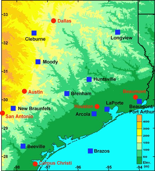
D00F13                              PARRISH ET AL.: TEXAQS II/GOMACCS OVERVIEW                                            D00F13

albeit related, issues. However, the distinction between their    Gammon et al., 2005a]. Light to moderate synoptic-scale
roles in these two issues is, at least in part, simply a matter   winds that oppose the direction of the bay breeze arising
of perspective and scale. Many of the chemical and mete-          in the late morning or early afternoon are particularly con-
orological processes that affect these two atmospheric            ducive to ozone formation and accumulation [Banta et al.,
species are important to both issues. For example, climate        2005; Ngan and Byun, 2008; Darby, 2005]. The stagnant
change is usually considered from a global viewpoint where        conditions that arise from the interaction of these two
intercontinental transport of ozone and aerosols determines       forces allow ozone precursors to accumulate and react
their impact. However, intercontinental transport is either       during the warmest and sunniest portion of the day. Later
the starting point or the end point of regional air quality       in the afternoon, the southerly Gulf breeze can advect the
concerns, since any particular region contributes outflow to      pool of high ozone across the city [Darby, 2005; Banta et
and receives inflow from that transport. This interrelation-      al., 2005].
ship of air quality and climate change issues was a founda-         [9] High concentrations of light alkenes such as propene,
tion of the 2004 International Consortium for Atmospheric         ethene, 1, 3-butadiene and butenes have been observed in
Research on Transport and Transformation (ICARTT) study           the Houston metropolitan area, and are closely associated
[Fehsenfeld et al., 2006]. The TexAQS/GoMACCS inten-              with petrochemical industry facilities in eastern Harris
sive in 2006 continues this approach; the instrumentation         County, Galveston County, Chambers County, and Brazoria
and deployment of many of the measurement platforms               County [Ryerson et al., 2003; Daum et al., 2003, 2004;
were planned to simultaneously address the issues involved        Berkowitz et al., 2004, 2005; Kleinman et al., 2002, 2003,
in both air quality and climate change.                           2005; Jobson et al., 2004; Karl et al., 2003; Buzcu and
  [4] The topics addressed in the present study have a long       Fraser, 2006; Xie and Berkowitz, 2006, 2007; Kim et al.,
history. There have been several previous studies conducted       2005]. These compounds collectively labeled as highly
in the Texas area. To place the current study into perspec-       reactive volatile organic compounds (HRVOC), and they
tive, section 2 provides a brief review of related previous       play a major role in forming the highest concentrations of
research, most notably the TexAQS 2000 study, which was           ozone observed in the Houston area [Ryerson et al., 2003;
a direct predecessor of the present field campaign.               Daum et al., 2003, 2004; Kleinman et al., 2002, 2005; Wert
  [5] The goal of this special journal section is to report       et al., 2003; Czader et al., 2008]. Historical analyses of
many of the TexAQS II/GoMACCS results. The ‘‘Final                routinely collected VOC data indicate that these compounds
Rapid Science Synthesis Report: Findings from the Second          are present in high concentrations on a routine basis in the
Texas Air Quality Study’’ (http://www.tceq.state.tx.us/           Houston area [Hafner Main et al., 2001; Estes et al., 2002;
assets/public/implementation/air/am/texaqs/rsst_final_            Brown and Hafner Main, 2002; Brown et al., 2002; Brown
report.pdf) presented an early summary of some of the             and Hafner, 2003; Kim et al., 2005; Buzcu and Fraser,
important findings that were judged to be particularly            2006; Xie and Berkowitz, 2006, 2007]. Consequently, the
important for air quality control policy decisions. This          high HRVOC concentrations observed during the two field
document will be referenced below as RSS Final Report.            study periods in 2000 and 2006 are not anomalously large,
  [6] The overall TexAQS II/GoMACCS study has several             and the conclusions drawn from those data should be
individual component programs that have their own goals           generally applicable to the Houston area.
and objectives; these separate components are briefly               [10] Field study results from 2000 indicate that indus-
described in section 3. Section 4 describes the meteoro-          trial emissions of HRVOC have been underreported in
logical conditions under which the measurements took              Houston [Ryerson et al., 2003; Wert et al., 2003; Xie and
place, and section 5 highlights some of the particularly          Berkowitz, 2007; Karl et al., 2003]. Results from more recent
important findings. The TexAQS II Radical and Aerosol             studies indicate that these emissions are still underreported
Measurement Project (TRAMP) is part of TexAQS II/                 [Robinson et al., 2008; Mellqvist et al., 2007; Smith and
GoMACCS, but will publish their results in a separate             Jarvie, 2008]. Source apportionment studies have been
special section in Atmospheric Environment.                       performed for VOC observations using TexAQS 2000 data
                                                                  [Karl et al., 2003; Zhao et al., 2004] and routine VOC
                                                                  measurements [Buzcu and Fraser, 2006; Buzcu-Guven and
2. Review of Previous Research Related to                         Fraser, 2008; Xie and Berkowitz, 2006, 2007; Wittig and
TexAQS II/GoMACCS                                                 Allen, 2008; Kim et al., 2005; Hafner Main et al., 2001;
  [7] Much of the previous research on air quality in the         Brown and Hafner Main, 2002; Brown and Hafner, 2003].
eastern Texas region has been supported through contracts         These studies have verified that the observed HRVOC are
with the Texas Commission on Environmental Quality                strongly associated with industrial emissions, and the studies
(TCEQ) and the Texas Environmental Research Consortium            have identified specific areas from which the highest
(TERC). The results of this contract research are often not       HRVOC emissions are emanating. The research efforts have
available in peer-reviewed publications. In such cases            not yet been able to precisely quantify the actual emissions
reports to the funding agency are referenced here to provide      occurring on a long-term basis from the underreported
the interested reader access to this work.                        sources. Mellqvist et al. [2007] and Robinson et al. [2008]
                                                                  have had some success in measuring emission fluxes from
2.1. Observational Studies of Ozone Formation in the              industrial point sources, but their efforts have been limited to
Houston Area                                                      small areas and short time frames. Both of these flux studies
  [8] High ozone concentrations in Houston depend strongly        have verified that industrial point source emissions for the
upon the interaction of synoptic-scale winds and local            areas studied are underreported at least part of the time, by
coastal/sea breeze oscillations [Banta et al., 2005; Nielsen-     factors approaching or exceeding an order of magnitude.

                                                             2 of 28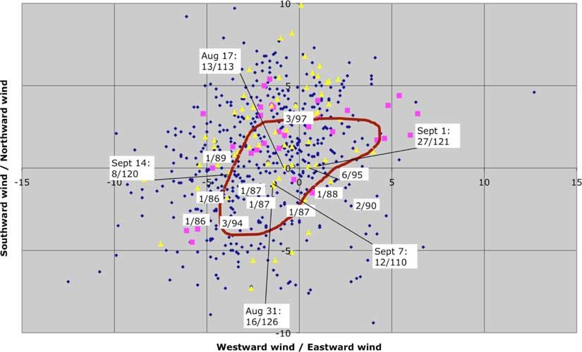
D00F13                               PARRISH ET AL.: TEXAQS II/GOMACCS OVERVIEW                                            D00F13

  [11] Actual emissions from industrial facilities may vary        tceq.state.tx.us/implementation/air/sip/dec2002hgb.html#docs,
considerably, owing to periodic or sporadic changes in             http://www.tceq.state.tx.us/implementation/air/airmod/docs/
processes, variations in control efficiency, and accidental        hgmcr_tsd.html, http://www.tceq.state.tx.us/implementation/
or planned releases. Mellqvist et al. [2007] found that the        air/sip/dec2004hgb_mcr.html, http://www.tceq.state.tx.us/
ethene emission flux near the Houston Ship Channel varied          implementation/air/airmod/data/hgb1.html#docs, http://www.
by a factor of 10 within 30 min, and smaller variations were       tceq.state.tx.us/implementation/air/airmod/data/hgb2.html,
common from day to day for propene and total alkanes.              www.tceq.state.tx.us/assets/public/implementation/air/sip/
However, the exact degree of variation of these emissions,         hgb/hgb_sip_2006/06027SIP_proCh2.pdf, and www.tceq.
and the quantity, composition and locations of sporadic            state.tx.us/assets/public/implementation/air/sip/hgb/hgb_sip_
emissions have not been well quantified. They could                2006/06027SIP_proCh3.pdf). Other modeling efforts have
account for a relatively large portion of the total annual         tested different chemical mechanisms in Houston’s photo-
emissions, on the basis of industry-supplied emission              chemical grid modeling, in order to study the effects of
reports [Murphy and Allen, 2005; Webster et al., 2007],            using different mechanisms on ozone model performance
but since the reported point source inventory is inconsistent      and control strategy effectiveness [Byun et al., 2005b;
with observations, and thus is inadequately quantified, it is      Faraji et al., 2008; Czader et al., 2008]. Modeling sensi-
difficult to reach a definitive conclusion.                        tivity studies have also been performed to guide selection of
  [12] High concentrations of HRVOC are capable of                 model parameters such as vertical mixing schemes, number
creating high concentrations of ozone. In Houston, ozone           and depth of model layers, and horizontal grid resolution
forms rapidly and efficiently in plumes of HRVOC and NOx           [Kemball-Cook et al., 2005; Byun et al., 2005b, 2007; Bao et
coemitted from industrial sources [Daum et al., 2003, 2004;        al., 2005]. TCEQ has supported photochemical modeling
Wert et al., 2003; Ryerson et al., 2003; Kleinman et al.,          efforts since 2000; additional reports can be found at http://
2002, 2005]. The highest ozone observed in Houston is              www.tceq.state.tx.us/implementation/air/airmod/project/
almost exclusively associated with industrial emission             pj_report_pm.html and at http://www.tercairquality.org/
plumes [Daum et al., 2004; Ryerson et al., 2003; Berkowitz         AQR/Projects/Modeling.
et al., 2004].                                                       [16] Mesoscale meteorological modeling is used to drive
  [13] When the United States moved from a standard                the photochemical grid models, and many studies have been
based on relatively high maximum 1-h average concen-               done to examine and reduce the uncertainties in these
trations (120 ppbv) to ones based on much lower maximum            models as well. One of the most successful efforts sought
8-h average concentrations (80 ppbv in 1997 and 75 ppbv in         to improve meteorological simulations of ozone episodes
2008) it became clear that the ozone transported into an           using radar profiler and other upper level wind data to
urban area can contribute significantly toward an exceed-          nudge met modeling [Nielsen-Gammon et al., 2007; Zhang
ance. Nielsen-Gammon et al. [2005b] reported that back-            et al., 2007; Stuart et al., 2007; Bao et al., 2005; Fast et al.,
ground ozone concentrations in southeast Texas average             2006]. Other efforts improved land cover data and land
about 50 ppbv, with higher concentrations observed with            surface modeling [Byun et al., 2005a; Cheng and Byun,
flow from the continental United States, and much lower            2008; Cheng et al., 2008], and studied the sensitivity of
concentrations observed with flow directly from the Gulf of        ozone simulations to solar irradiance and photolysis rates
Mexico.                                                            [Zamora et al., 2005; Fast et al., 2006; Pour-Biazar et al.,
                                                                   2007; Byun et al., 2007; Koo et al., 2008]. TCEQ has
2.2. Photochemical Modeling of Ozone Formation in                  supported mesoscale meteorological modeling efforts by
the Houston Area                                                   Nielsen-Gammon and others since 2001; 25 reports about
                                                                   mesoscale meteorological modeling in Houston have been
  [14] Photochemical grid modeling of the Houston area             provided to TCEQ, and can be found at http://www.tceq.
has been challenging owing to the complex coastal wind             state.tx.us/implementation/air/airmod/project/pj_report_
circulation, the complex petrochemical point emission sour-        met.html#met02.
ces in Harris, Galveston, Chambers, and Brazoria Counties,
and the routine challenges associated with modeling a
metropolitan area of over five million inhabitants. One of
the purposes of the TexAQS 2000 and TexAQS II field                3. Components of TexAQS II/GoMACCS
studies was to address the uncertainties that affect photo-          [17] Sections 3.13.6 describe the principal goals and
chemical grid modeling and its regulatory applications. The        resources contributed by the independent programs that
insights gleaned from the TexAQS 2000 and subsequent               constituted the larger, 2-year TexAQS II/GoMACCS field
studies have helped resolve some of these uncertainties.           program. Appendices A and B give more experimental
  [15] Several studies have endeavored to identify and             details of the individual platforms and sites. In addition to
reduce the uncertainties in the Houston photochemical grid         the research that is described in this special section, the
modeling. Foremost among these efforts are the studies that        program also included work conducted by other groups. The
have sought to quantify underreported industrial HRVOC             Air Quality Research program of TERC funded much of
emissions [Ryerson et al., 2003; Wert et al., 2003; Xie and        this additional work, including the TexAQS II Radical
Berkowitz, 2007; Yarwood et al., 2004; Webster et al., 2007;       Measurement Project (TRAMP), the Northeast Texas
Smith and Jarvie, 2008] and to assess the sensitivities of ozone   Plume Study (NETPS), the TexAQS II Tetroon Campaign,
simulations to the underreporting of these emissions [Byun et      research flights of the Baylor University Piper Aztec aircraft
al., 2007; Jiang and Fast, 2004; Nam et al., 2006] (see also       and the Houston Triangle Experiment. More information can
TCEQ Houston-Galveston-Brazoria online reports: http://www.

                                                             3 of 28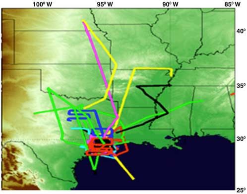
D00F13 PARRISH ET AL.: TEXAQS II/GOMACCS OVERVIEW D00F13
be found at the TERC website: http://www.tercairquality. situ measured CCN behavior of the ambient aerosol be
org/AQR/. replicated on the basis of measured aerosol size distribution
and composition? This question is of special interest in a
3.1. TexAQS 2006 and Gulf of Mexico Atmospheric heavily polluted urban area like Houston. (2) To what extent
Composition and Climate Study (NOAA) can theoretical aerosol-cloud activation models predict
[18] The NOAA WP-3D and Twin Otter Lidar aircraft cloud droplet number concentrations, given measurements
combined with the Research Vessel Ronald H. Brown and of aerosol size and composition? (3) To what extent do
the radar wind profiler network to conduct the combined measured radiative fluxes above and below cloud agree with
TexAQS 2006/GoMACCS study. The WP-3D mapped trace those predicted on the basis of atmospheric radiative trans-
gases, aerosols and radiative properties over the eastern fer models? (4) To what extent can evidence of aerosol
Texas region and the Lidar aircraft, mapped the regional effects on cloud microphysics, precipitation initiation and
distribution of boundary layer ozone, aerosols and mixing cloud radiative properties be observed? (5) How does
layer heights in the same region. The Ronald H. Brown used entrainment influence cloud microphysics? (6) To what
both in situ and remote atmospheric sensors to examine extent can large eddy simulation (LES) of cloud fields predict
low-altitude outflow of pollution from eastern Texas and the statistical properties of those measured? (7) Can the
the chemical environment of the Texas Gulf Coast region. sources and character of the organic portion of the Houston
The Radar Wind Profiler Network included ten sites that aerosol be understood? (8) What processes govern the
measured vertical profiles of boundary layer winds (see evolution of aerosols as they are advected from source-rich
Appendix B), which provided information on regional-scale areas?
trajectories and transport of air masses. The science plan that
describes the research aims of Texas 2006/GoMACCS can 3.4. Satellite Data Integration (NASA, NOAA,
be found at http://esrl.noaa.gov/csd/2006/. and TCEQ)
[21] Scientists from a number of NASA and NOAA
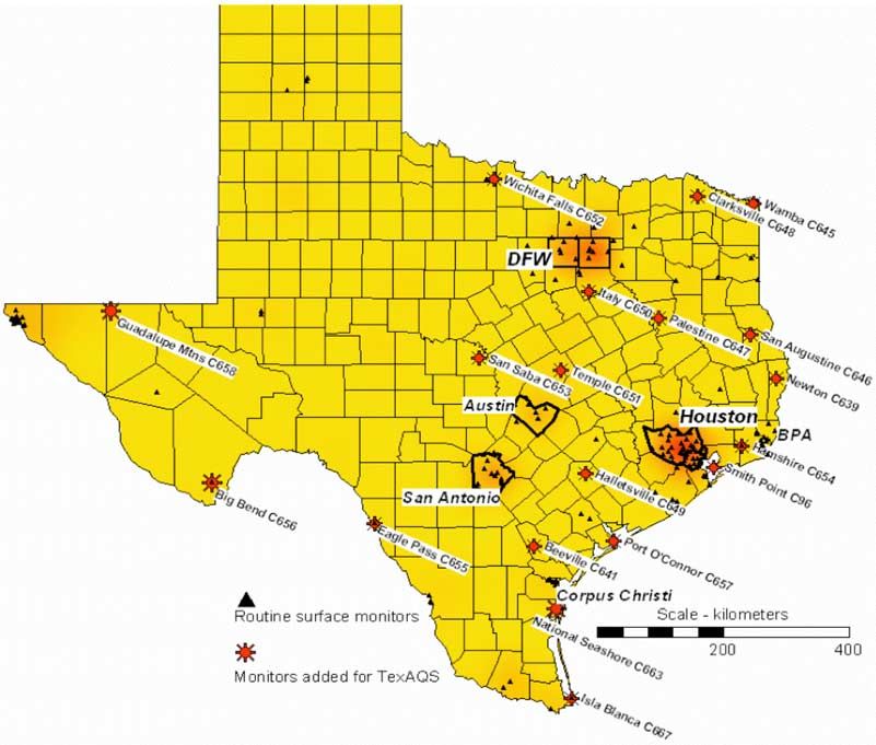
3.2. Ground Site Network (TCEQ, University of Texas, satellite groups participated in the TexAQS/GoMACCS
and Texas A&M University) field mission. The satellite component contributed to flight
[19] TCEQ maintains a network of almost 100 ground planning activities and integrated measurement and model-
stations in eastern Texas that measure and archive concen- ing studies focusing on influences of continental-scale
trations of air pollutants and meteorological data (data are processes on regional air quality within east Texas. Airborne
available at the TCEQ web monitoring operations web site: and surface measurements were used to verify chemical and
http://www.tceq.state.tx.us/compliance/monitoring/air/ aerosol analyses and to validate satellite observations on
monops/hourly_data.html). These sites are operated to assess local scales. Ensemble trajectories (sampling analyzed
compliance with National Ambient Air Quality Standards, chemical and aerosol fields to account for chemical trans-
and consequently the measurements are primarily focused formation during transport) were used to identify source
on concentrations of ozone, particulate matter, and their regions of pollution sampled by the airborne and surface
precursors. They are located almost exclusively in urban sensors. Satellite measurements were used to constrain the
areas where the potential for human exposures to these air chemical and aerosol analyses, quantify source strengths
pollutants is greatest. For TexAQS II, additional sites were and verify model predictions on a regional to global scale.
deployed to provide a combination of upper air meteoro- [22] Satellite instruments are currently able to observe
logical information and surface concentrations of air pollu- several criteria pollutants in the troposphere including ozone
tants in rural areas. More details of these specially deployed (O3), nitrogen dioxide (NO2), carbon monoxide (CO), sulfur
sites are given in the descriptions of the Radar Wind Profiler dioxide (SO2) and aerosol optical depth (AOD) (Table A8 in
Network and the Surface Air Quality Monitoring Network Appendix A). Satellites also provide retrievals of atmo-
in Appendix B. The goal of these additional sites was to spheric thermodynamic properties (temperature, moisture,
characterize boundary layer meteorology and surface air and clouds) as well as surface and top of atmosphere (TOA)
quality for the assessment of regional air pollutant transport. radiative fluxes. Polar-orbiting satellites (e.g., Terra, Aqua,
Finally, Texas A&M University operated a flux tower with Aura, and the National Polar-Orbiting Operational Environ-
measurements of key constituents in Lick Creek Park, just mental Satellite, or POES) provide global coverage once per
south of College Station, Texas. day and offer a unique vantage point for observing inter-
continental pollution transport. Geostationary satellites
3.3. TexAQS 2006/GoMACCS Aerosol-Cloud Study (e.g., Geostationary Operational Environmental Satellite,
(National Science Foundation and NOAA) or GOES) provide coverage over the continental United
[20] The CIRPAS Twin Otter aircraft was the primary States once every fifteen minutes and are useful for follow-
platform for the aerosol-cloud study. The major scientific ing continental-scale pollution transport and regional pollu-
objectives centered on the relationship between aerosol tion events. Satellite tropospheric trace gas and aerosol
physical and chemical properties and the microphysical retrievals and area-burned estimates provide valuable infor-
and radiative properties of the clouds. Therefore, this mation for emission modeling. Long-term, space-based
experiment represents a continuing effort to obtain detailed, observations place airborne measurements obtained during
in situ field data that will aid in understanding the indirect limited duration field experiments within the context of
climatic effect of aerosols. In addition, there was focus on observed interannual variability and trends.
understanding the atmospheric evolution of aerosols. Spe- [23] The availability of near-real-time (within 12– 24 h)
cific scientific questions included: (1) To what extent can a satellite data significantly increased the role of satellite
CCN closure be accomplished; that is, how closely can in data in flight planning during TexAQS/GoMACCS. High
4 of 28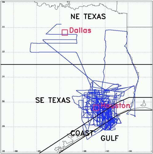
D00F13                               PARRISH ET AL.: TEXAQS II/GOMACCS OVERVIEW                                         D00F13

temporal resolution Step and Stare profile retrievals of           to identify aerosol type. The aerosol intensive parameters
tropospheric O3 and CO profiles from the Tropospheric              measured by the HSRL (extinction/backscatter ratio, back-
Emission Spectrometer (TES) [Beer, 2006] were available            scatter wavelength dependence, depolarization) provided a
for studying boundary layer exchange processes. 500 mb CO          means to identify various aerosol types and investigate the
retrievals from the Atmospheric Infrared Sounder (AIRS)            vertical and horizontal variability of aerosol types in the
[McMillan et al., 2005] provided a regional context for            TexAQS/GoMACCS study region, and to determine how
interpretation of ground and airborne measurements. The            aerosol optical thickness was distributed among the various
Multiangle Imaging SpectroRadiometer (MISR) [Diner et              aerosol types.
al., 1998] provided retrievals of AOD and aerosol type.              [29] 4. Characterize the behavior and variability of the
Aerosol attenuated backscatter measurements from the Cloud         planetary boundary layer (PBL) height. Lidar systems have
Aerosol Lidar with Orthogonal Polarization (CALIOP) instru-        been widely used to examine the structure and variability of
ment onboard the Cloud-Aerosol Lidar and Infrared Path-            the PBL top and to derive the entrainment zone depth [e.g.,
finder Satellite Observation (CALIPSO) satellite [Winker et        Cohn and Angevine, 2000; Brooks, 2003]. Since the King
al., 2007] were used to identify the altitude and thickness        Air flew at high (9 km) altitude exclusively, the lidar
of regional- and continental-scale aerosol plumes. GOES            measurements featured long, uninterrupted observations of
Aerosol/Smoke Product (GASP) AOD [Knapp et al., 2002]              the PBL and entrainment zone.
and GOES visible imagery [Gurka et al., 2001] characterized          [30] 5. Assess model simulations of aerosol extinction
transport of aerosol and smoke plumes. GOES Wildfire               profiles. The vertical profiles of aerosol extinction and
Automated Biomass Burning Algorithm (WF-ABBA) [Prins               aerosol intensive parameters measured by the HSRL were
et al., 1998] and MODIS [Giglio et al., 2003] fire detections      used to help evaluate the ability of models to reproduce
were used to identify biomass burning sources and provide          aerosol extinction profiles and optical thickness.
area-burned estimates for wild fire emissions modeling.
  [24] The availability of real-time (within 0– 3 h) satellite     3.6. IONS-06NASA
trace gas and aerosol retrievals allowed chemical and                [31] In support of TexAQS II, IONS-06 operated 22
aerosol assimilation/forecast systems to be used for flight        sounding stations (Table A9 in Appendix A) to provide
planning activities during TexAQS/GoMACCS. Total col-              consistently located vertical profiles of ozone concentration
umn ozone retrievals from the Ozone Monitoring Instru-             over Houston and beyond [Thompson et al., 2008]. IONS-06
ment (OMI) [Levelt et al., 2006a, 2006b] and AOD                   was strategically configured to align a group of sites along
retrievals from the Moderate Resolution Imaging Spectror-          important transport pathways, i.e., Pacific to western U.S.
adiometer (MODIS) instruments [Kaufman et al., 1997]               coast, southwest United States and Mexico toward Houston,
provided for real-time chemical and aerosol data assimila-         Gulf coast and Caribbean toward Houston, and Houston
tion/forecasting activities. The use of satellite, aircraft, and   toward Huntsville, Alabamanortheastern North America
surface measurements, in conjunction with advanced mod-            [Cooper et al., 2007]. At Houston, there were two IONS-06
eling techniques, supports the development of an Air               sampling venues during TexAQS 2006. Launches by G. A.
Quality Assessment and Forecasting capabilities under the          Morris et al. (An evaluation of the influence of the morning
U.S. Integrated Earth Observation System (http://usgeo.gov/        residual layer on afternoon ozone concentrations in Houston
docs/EOCStrategic_Plan.pdf).                                       using ozonesonde data, submitted to Atmospheric Envi-
                                                                   ronment, 2009) were performed at the University of
                                                                   Houston (29.7°N, 95.4°W) not far from downtown Houston,
3.5. Airborne High Spectral Resolution Lidar Aerosol               17 August to 5 October 2006. Sondes were also launched
Investigations (NASA)                                              from the R/V Ronald H. Brown during August along its
  [25] During TexAQS/GoMACCS, the NASA Langley                     cruise track; this series continued through 11 September
Research Center (LaRC) airborne High Spectral Resolution           2006 [Thompson et al., 2008].
Lidar (HSRL) was deployed on the NASA B200 King Air
aircraft to measure profiles of aerosol extinction, back-
scattering, and depolarization. These measurements were
                                                                   4. Meteorological Context of TexAQS II/
acquired to address several objectives:
  [26] 1. Map the vertical and horizontal distributions of         GoMACCS
aerosols during transport downwind from major sources.               [32] The entire period of TexAQS II (1 June 2005 to
The HSRL profiles provided ‘‘curtains’’ showing the aero-          18 October 2006) was unusually dry for the state of Texas
sol distributions below the aircraft. Since the lidar measure-     as a whole. Drought was widespread November 2005 until
ments clearly depict the altitudes of aerosol layers, they         January 2007. However, Southeast Texas and the coastal
were used to indicate the height to which aerosols are             portions of Texas was one of the few areas spared the
injected into the atmosphere, which is important for mod-          unusual drought conditions. Figure 1 shows drought con-
eling the long-range transport of aerosols.                        ditions across Texas at the beginning and end of TexAQS
  [27] 2. Evaluate measurements from the CALIOP sensor             2006/GoMACCS intensive field activities of 2006. The
on the CALIPSO satellite. HSRL backscatter, extinction, and        drought reached its peak during late August and early
depolarization profiles were used to evaluate the CALIOP           September 2006, after which rains helped mitigate conditions.
calibration, as well as the level 1 (attenuated backscatter),      While Houston avoided drought conditions, the Dallas–Fort
and level 2 (aerosol backscatter, aerosol extinction) profiles.    Worth area was remarkably dry. In August 2006, Bush
  [28] 3. Provide profiles of aerosol extinction, backscatter      Intercontinental Airport in Houston (IAH) was 0.6°C above
and depolarization and investigate the use of these profiles       normal, with 89% of normal rainfall, while DallasFort

                                                             5 of 28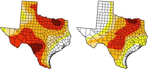
D00F13                              PARRISH ET AL.: TEXAQS II/GOMACCS OVERVIEW                                         D00F13

                                                                  unusually high temperatures that culminated in numerous
                                                                  records being broken. By comparison, the TexAQS II/
                                                                  GoMACCS period was close to normal in the Houston area
                                                                  with respect to both temperature and precipitation.
                                                                    [34] Typically during August and September, the strong
                                                                  southerly winds of midsummer begin to weaken and cold
                                                                  fronts penetrate southward farther and farther into Texas.
                                                                  Behind the cold fronts, northeast winds tend to bring
                                                                  polluted air from the central and eastern United States.
                                                                  The extent of transport from the northeast controls back-
                                                                  ground ozone levels, while enhancement of ozone due to
Figure 1. Drought conditions in Texas on (left) 1 August          local emissions depends on the lightness of the winds
2006 and (right) 10 October 2006, as depicted by the U.S.         [Nielsen-Gammon et al., 2005a, 2005b]. Mean winds do
Drought Monitor. The range of colors from white to dark           not tell the whole story; often just a few days can make an
red correspond to no drought, incipient drought, moderate         ozone season exceptionally bad.
drought, severe drought, extreme drought, and exceptional           [35] To help characterize the wind conditions during
drought.                                                          TexAQS 2006/GoMACCS, Figure 2 shows the mean wind
                                                                  conditions for each day during the field intensive, 1 August
                                                                  2006 through 15 October 2006. Winds are represented as
Worth International Airport (DFW) was 3.0°C above normal,         daily mean winds from buoy 42035, located just offshore
with only 26% of normal rainfall. September was a more            from Galveston. Each day’s wind is represented by its mean
typical month: IAH saw temperatures 0.5°C above normal            westerly (u) and southerly (v) values, so that a vector drawn
with 74% of normal rainfall, while DFW saw temperatures           from the origin to a given symbol depicts the wind speed
0.1°C above normal with 107% of normal rainfall.                  and direction for that symbol. The winds during the field
  [33] Meteorological differences yield differences in air pol-   intensives of TexAQS 2000 and 2006 are compared with all
lution characteristics between TexAQS 2000 and TexAQS II.         winds from 1998 through 2006, 1 August through 15 October
TexAQS 2000 took place during a period of substantial             (blue diamonds) and days with an 8-h maximum ozone
drought in southeast Texas, and the very end of August and        greater than 85 ppbv are identified.
the first few days of September were characterized by               [36] The distribution of winds during the 2006 field
                                                                  intensive broadly matches the climatology, except for a

         Figure 2. Wind conditions during 1 August through 15 October 1998 – 2006. Each dot represents the
         24-h mean wind measured at Buoy 42035, just offshore of Galveston. The westerly (u) and northerly (v)
         wind components are given along the x and y axes, respectively; a dot in the northeast quadrant, for
         example, corresponds to a wind blowing from southwest to northeast. Pink squares are winds during
         TexAQS 2000. Yellow triangles are winds during TexAQS 2006/GoMACCS. Text insets give number of
         stations in 2006 exceeding an 8-h ozone average of 85 ppb and the maximum value of 8-h ozone average
         (ppbv). Dates are given for exceedances of over 100 ppbv. The maroon curve indicates the approximate
         area of winds conducive to high ozone during 1998– 2004.

                                                             6 of 28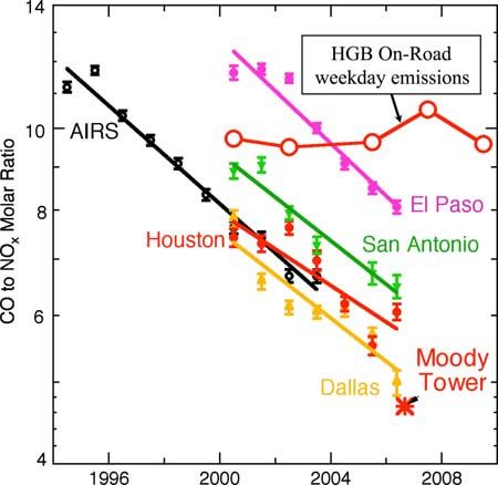
D00F13                              PARRISH ET AL.: TEXAQS II/GOMACCS OVERVIEW                                          D00F13

surplus of strong winds from the south (yellow triangles near    sources near Houston, Texas: a laser photoacoustic spec-
the top center of Figure 2) and a deficit of strong winds from   troscopy (LPAS) instrument on board the WP-3D aircraft
the east (lack of yellow triangles near the left of Figure 2).   [de Gouw et al., 2009] and a solar occultation flux (SOF)
The situation less closely resembles that of TexAQS 2000.        instrument operated in a mobile laboratory (J. Mellqvist et
TexAQS 2006 did not experience any analogs to the strong         al., Measurements of industrial emissions of alkenes in
westerly flow of 30 August 30 to 1 September 2000                Texas using the Solar Occultation Flux method, submitted
(rightmost pink squares), and conversely, TexAQS 2000            to Journal of Geophysical Research, 2009). The latter
experienced almost no light winds from the northeast even        instrument also measured propene and total alkane fluxes.
though they were common during TexAQS 2006 and in                Both instruments repeatedly quantified ethene fluxes from
general.                                                         the Mont Belvieu chemical complex to the northeast of
  [37] The maroon line in Figure 2 depicts the margins of        Houston, one of the largest emission sources in the Houston
wind conditions that were favorable for high ozone during        area. The results from the LPAS (520 ± 140 kg h1) during
TexAQS 2000. Within this line, the only conditions that          10 different WP-3D flights agreed well with those from
occurred in both 2000 and 2006 are light winds from the          6 independent measurements by the SOF (440 ± 130 kg h1).
southeast. In 2000, one such day, 25 August, produced very       Two considerations can serve to put these fluxes in per-
high ozone concentrations. Yet, in 2006, few such days           spective. First, the 2006 TCEQ point source database
resulted in high ozone. A check of individual days (not          estimated the total ethene emissions from Mont Belvieu to
shown) indicates that most of these days involved wide-          be 81 kg h1, a factor of 5 to 7 lower than the measured
spread rain or cloudiness in 2006, suppressing what would        fluxes. Similar discrepancies are generally found throughout
otherwise be favorable ozone formation conditions.               the industrial facilities in the Houston area; Mellqvist et al.
  [38] The highest levels of ozone within the Houston area       (submitted manuscript, 2009) found that for all measure-
during TexAQS 2006 occurred on four Thursdays (17 August,        ments during the campaign, the 2006 emission inventory
31 August, 7 September, and 14 September) and one Friday         underestimated the measured fluxes by an average factor of
(1 September). As suggested by the mean wind on 1 September      10 for ethene and 11 for propene. Second, Murphy and
being almost directly opposite the mean wind on 31 August,       Allen [2005] investigated the role of large, accidental
there is some evidence that pollutants from 31 August may        releases of HRVOC in ozone formation in the HGB area,
have recirculated back into parts of Houston on 1 September.     and identified 763 HRVOC emission events in a 1-year
The mean wind on 17 August was also sufficiently close to        period. More than half of these events released less than
zero that some recirculation may have been possible under        454 kg total HRVOC. Thus, the Mont Belvieu complex
the influence of the sea breeze. In general, though, the high-   routinely emits more ethene each hour than the total
ozone events during 2006 were less directly influenced by        HRVOC released in the majority of the individual accidental
the sea breeze than those of 2000.                               release events considered by Murphy and Allen [2005]. The
  [39] Although no high-ozone days occurred in both 2000         emissions from these facilities represent a much larger
and 2006 under similar meteorological circumstances, the         source of HRVOC and much more substantial contribution
combined records from 2000 and 2006 together encompass           to ozone formation than indicated by current emission
all common wind scenarios for high ozone in the Houston          inventories.
area.                                                              [43] Results from four different observationally based
                                                                 analyses (ethene/NOx emission ratios in plumes from petro-
                                                                 chemical facilities, the ambient distribution of ethene con-
5. Overview of Results                                           centrations, the ambient distribution of formaldehyde, and
  [40] This section presents an overview of the some of the      long-term auto-GC ethene measurements) all show evidence
important results of the TexAQS II/GoMACCS field study,          for a significant decrease in ethene emissions in the Greater
including those published in this special journal section,       Houston area between the TexAQS 2000 and TexAQS II
published elsewhere, and emerging in manuscripts that are        studies [Gilman et al., 2009] (see also RSS Final Report).
still in preparation. Some additional results are described      The weight of evidence from these four analyses indicates
that are presently not included in any planned publications,     that ethene emissions from the petrochemical facilities
but are discussed here to give a complete overview of the        decreased by about 40(±20)% (i.e., approximately a factor
observational programs involved in TexAQS II/GoMACCS.            of 1.7) between 2000 and 2006.
                                                                   [44] A remarkable finding of the TexAQS II study is that
5.1. Observational Tests of Emission Inventories                 the underestimate of emission fluxes of HRVOC from
  [41] Air quality and climate change problems originate         petrochemical facilities established by the TexAQS 2000
from society’s increased emissions of air pollutants and their   study has not yet been fully integrated into inventories
precursors (VOC, NOx, SO2, CO, air toxics) and radiative         developed since that study. The TexAQS 2000 study estab-
forcing agents (CO2, CH4, N2O, halocarbons, black carbon,        lished that inventories underestimated these emissions by
aerosols). Our understanding of these emissions on both          1 – 2 orders of magnitude [Ryerson et al., 2003]. In an
regional and global scales is critically limited. The data       analysis prepared for the RSS Final Report, John Jolly of
collected during this field study provide tests of emission      TCEQ reported that total HRVOC emissions included in the
inventories, some of which are summarized here.                  Harris County Point Source emission inventory for 2000–
5.1.1. Emissions of VOC From Petrochemical Facilities            2004 were fairly steady across those years, with the lowest
in the Houston Area                                              year (2002, at 3300 tons) being about 83 percent of the
  [42] Two independent techniques were deployed during           highest year (2004, 4000 tons). Mellqvist et al. (submitted
TexAQS 2006 to quantify fluxes of ethene from industrial         manuscript, 2009) show that there have been some recent,

                                                            7 of 28
D00F13 PARRISH ET AL.: TEXAQS II/GOMACCS OVERVIEW D00F13
VOCs served to sustain elevated levels of OH reactivity
throughout the time of peak ozone production.
5.1.2. On-Road Mobile Emission Inventories in the
Houston Area
[46] Figure 3 compares CO to NOx ratios from ambient
measurements collected during the morning rush hour travel
peak with those from emission inventories. The data are
treated as described by Parrish [2006]. The Dallas and
Houston routine ambient data are in excellent agreement
with the nationwide AIRS data. The TexAQS 2006 ratio
derived from the TRAMP measurements made at the
Moody Tower site (B. Lefer, private communication,
2007) agree reasonably well with the routine monitoring
data. The ratios in El Paso and San Antonio are significantly
higher, which is attributed to the older vehicle fleets found
in those urban areas.
[47] In Figure 3 the Houston area (indicated as HGB)
inventory overestimates the CO to NOx emission ratio, and
that overestimate becomes worse with time as the inventory
does not show a significant temporal decrease. It should be
Figure 3. Measured CO to NOx ratios (solid symbols noted that the on-road emissions inventory value for 2000
color-coded according to area) in four Texas urban areas was calculated with actual data for 2000, whereas the on-road
during the morning traffic peak (0600 to 0900 local standard mobile inventories for later years are less certain projections.
time) compared to the ratio from on-road mobile emissions Parrish [2006] showed that nation-wide the rapid decrease
from the HGB emission inventory (open symbols). The (6.6%/a) in the CO to NOx ratio is partially due to a slower
black symbols give the average ratio for all stations in the decrease in CO emissions (4.6%/a), which implies a signif-
EPA AIRS network from Parrish [2006]. icant increase in NOx emissions (approximately 2%/a). The
large inventory overestimate in the ratio in 2006 is attributed
to a factor of 2 overestimate in CO emissions, and an under-
relatively small systematic increases in the inventoried estimate in present NOx emissions. This causes NOx to CO
HRVOC emissions; the last eight entries in their Table 3 emission ratios in urban areas, which are often dominated by
indicate that inventoried ethene and propene emissions from on-road mobile emissions, to be underestimated by current
a large majority of the petrochemical facilities in the Houston emission inventories.
area increased from 149 and 176 kg h1, respectively, in 2004 [48] Urban emission ratios sampled by the WP-3D air-
to 277 and 252 kg h1, respectively, in 2006. Thus, decreases craft in 2006 and the NCAR Electra aircraft in 2000 are
in actual HRVOC emissions and some increases in inventory consistent with measurements carried out at a Houston
estimates have improved the accuracy of the emission highway tunnel in 2000 [McGaughey et al., 2004]. These
estimates, but importantly, inventories still underestimate measurements demonstrate the weekday increase in CO/
HRVOC emissions by 1 order of magnitude. CO2 and CO/NOx emission ratios from midday to the
[45] A chemically diverse set of volatile organic com- afternoon rush hour correlated with increases in the propor-
pounds (VOCs) and other gas-phase species was measured tion of gasoline vehicles during rush hour. Similar to the
in situ aboard the NOAA R/V Ronald H. Brown as the ship routine monitors, the aircraft and tunnel observations indi-
sailed throughout the Houston and Galveston Bay area cate that inventories overestimate mobile source CO by at
(HGB) [Gilman et al., 2009]. The reactivities of CH4, least a factor of 2. Comparison of the 2000 and 2006 aircraft
CO, VOCs and NO2 with the hydroxyl radical, OH, were data suggests that urban CO emissions declined by roughly
determined in order to quantify the contributions of these a factor of 2 between the studies (using either CO2 or NOx
compounds to potential ozone formation. The total OH as a comparison) in agreement with the National Emission
reactivity was high in HGB, averaging 10 s1, primarily Inventories from 1999 and 2005, which show a similar
owing to the impact of industrial emissions. In comparison, decline (G. J. Frost et al., manuscript in preparation, 2009).
during ship-based measurements downwind from New York 5.1.3. Marine Vessel Emissions in the Texas Gulf
City and Boston in 2002, the total OH reactivity only very Coast Region
rarely exceeded 10 s1 [Goldan et al., 2004]. By compen- [49] Gaseous and particulate emissions from commercial
sating for the effects of boundary layer mixing, the diurnal marine shipping were investigated through measurements
profiles of the OH reactivity were used to determine the made in more than 200 exhaust plumes from a variety of
source signatures and relative magnitudes of biogenic, ships encountered by the Ronald H. Brown throughout the
anthropogenic (urban + industrial), and oxygenated VOCs Gulf Coast region of Texas including most of the major
as a function of the time of day. This analysis demonstrates ports and the Houston Ship Channel. Gas-phase and partic-
that the predominant source of formaldehyde to the air ulate emission factors were determined under actual oper-
masses sampled by the Ronald H. Brown in HGB was from ating conditions and compared with published emission
secondary production, with primary emissions playing only factors used for emission inventory modeling.
a minor role. The secondary formation of oxygenated VOCs [50] E. J. Williams et al. (Emissions of NOx, SO2, CO,
in addition to the continued emissions of anthropogenic H2CO and C2H4 from commercial marine shipping during
8 of 28D00F13 PARRISH ET AL.: TEXAQS II/GOMACCS OVERVIEW D00F13
TexAQS 2006, submitted to Journal of Geophysical High-time-resolution (1 s average) NH3 measurements
Research, 2009) show that bulk freighter and tankers were made from the WP-3D aircraft by a Chemical Ioniza-
emitted considerably more NO2 per unit fuel burned than do tion Mass Spectrometry technique [Nowak et al., 2007] and
underway container carriers, passenger vessels, or tugs. from the Ronald H. Brown by quantum cascade laser
Emission of SO2 was higher for all cargo vessels than for absorption (S. C. Herndon et al., manuscript in preparation,
passenger ships or tugs, which is due to the use of higher 2009) with the goals of characterizing sources and examin-
sulfur residual fuels by cargo ships and lower sulfur ing the effect of NH3 on atmospheric aerosol formation.
distillate fuels by passenger ships and tugs. There is broad [54] Mixing ratios measured aboard the WP-3D aircraft
general agreement between these data and published over the Houston urban area ranged from 0.2 to 3 ppbv, and
emission factors, although variability is large for both generally decreased with increasing altitude (J. B. Nowak et
cases. Marine vessel emission factors for NO2 and SO2 are al., manuscript in preparation, 2009). Though infrequent,
considerably larger than for stationary sources such as coal- plumes with NH3 mixing ratios from 5 to greater than
fired or gas-fired power plants, which indicates that 50 ppbv were observed in the boundary layer below 1 km
emissions from commercial marine vessels likely make altitude. Corresponding increases in fine particle volume
significant contributions in coastal areas and ports. and particulate nitrate (NO 3 ) and decreases in HNO 3
[51] Lack et al. [2008] measured particulate emission mixing ratios typically accompanied the large observed
factors for these same ships, and found the emission of NH3 enhancements. These correlated variations are consis-
black carbon (BC) from these diesel engine powered vessels tent with ammonium nitrate formation. NH3 mixing ratios
was a factor of 2 greater than previous estimates. They as high as several hundred ppbv were measured in the HSC
found that tugs emit more BC than do large cargo vessels, from the Ronald H. Brown. Up to this point, it has proven
which has particular significance for the Houston-Galveston difficult to trace the sources of plumes with high NH3
region since these vessels constitute a large fraction of total concentrations to particular industrial facilities.
ship traffic there. Lack et al. [2009] also found that the [55] Power plants that have installed Selective Catalytic
chemical composition (sulfate and organic material) and Reduction (SCR) units constitute a possible NH3 source.
aerosol properties such as single-scatter albedo and partic- This process adds aqueous NH3 to the exhaust gases as a
ulate water uptake of ship exhaust particulates was directly reagent to decrease NOx emissions. NH3 ‘‘slippage,’’ i.e.,
related to the fuel sulfur content. unwanted emissions of NH3 into the atmosphere, occurs
5.1.4. Biogenic Emissions in the Eastern Texas Region when exhaust gas temperatures are too low for the SCR
[52] C. Warneke et al. (Biogenic emission measurement reaction to proceed to completion, or when excess NH3 is
and inventories: Determination of biogenic emissions in the added. The W.A. Parish electric generating facility is
eastern United States and Texas and comparison with equipped with these units, and the WP-3D aircraft sampled
biogenic emission inventories, submitted to Journal of Geo- the Parish plume on numerous flights during TexAQS 2006.
physical Research, 2009) utilize airborne measurements of Clear enhancements of CO2, NOy, and SO2 were observed,
isoprene and monoterpenes conducted during the TexAQS but no difference in NH3 mixing ratios could be discerned
2006 campaign along with results from the SOS 1999, during the plume transect. The lack of NH3 enhancement in
TexAQS 2000, and ICARTT 2004 studies to evaluate the the power plant plumes sampled by the WP-3D indicates
biogenic emission models BEIS3.12, BEIS3.13, MEGAN2 that NH3 slippage was not significant during any of the
and WM2001. Two methods are used for the evaluation. TexAQS 2006 plume transects.
First, the emissions are directly estimated from the ambient
isoprene and monoterpene measurements assuming a well- 5.2. Air Quality: Measurements and Observational
mixed boundary layer and using calculated OH concentra- Based Analyses
tions, and are compared with the emissions from the
inventories extracted along the flight tracks using measured 5.2.1. Role of Nitrate Radicals and N2O5
light and temperature. Second, BEIS3.12 is incorporated [56] Hydrolysis of N2O5 provides a nonphotochemical
into the detailed transport model FLEXPART, which allows mechanism for conversion of NOx to soluble nitrate (NO 3)
the isoprene and monoterpene mixing ratios to be calculated that can be competitive with, or even exceed, photochemical
and compared to the measurements. The overall agreement oxidation of NO2 by OH. Formation of N2O5 proceeds
for all inventories is within a factor of two and both methods through oxidation of NO2 to NO3 by ozone and further
give consistent results. MEGAN2 is in most cases higher, reaction of NO3 with NO2. The process is only important in
and BEIS3.12 and BEIS3.13 lower than the emissions the dark because of the photochemical instability of NO3.
determined from the measurements. Regions with clear Hydrolysis of N2O5 occurs heterogeneously via uptake to
discrepancies are identified. For example, an isoprene hot aerosol. Its rate therefore depends on the availability of
spot to the northwest of Houston, Texas, is expected from aerosol surface area and on the heterogeneous uptake
BEIS3 but not observed in the measurements. Interannual coefficient of N2O5 to aerosol, g(N2O5). Both are highly
differences in emissions were also observed: the isoprene variable, making the dark loss of NOx more difficult to
emissions estimated from the measurements in Texas in accurately predict than the photochemical loss via OH
2006 may have been 50% lower than in 2000 under the reaction.
same light and temperature conditions. [57] Measurements of NO3 and N2O5 from the NOAA
WP-3D aircraft on night flights allowed the direct determi-
5.1.5. Ammonia Emissions in the Eastern Texas Region
nation of the overall loss rates for N2O5 and for its
[53] Ammonium nitrate aerosol is formed from the reac-
tion of gas-phase ammonia (NH3) and nitric acid (HNO3). heterogeneous uptake coefficient [Brown et al., 2009].
The g(N2O5) values derived from the field measurements
9 of 28D00F13 PARRISH ET AL.: TEXAQS II/GOMACCS OVERVIEW D00F13 were considerably smaller than predictions from current from petrochemical facilities located along the Houston ship model parameterizations based on laboratory data. The channel. result is consistent with the one set of previous aircraft determinations of N2O5 heterogeneous hydrolysis rates in 5.3. Air Quality: Meteorological and Modeling Studies the northeast United States [Brown et al., 2006], which 5.3.1. Interregional and Long-Range Transport showed small g(N2O5) on mixed organic/neutral ammonium [61] During the last decade, emission control measures sulfate aerosol. This aerosol type was prevalent during have successfully reduced the highest ozone concentrations TexAQS 2006. Lifetimes of N2O5 were long enough to observed in the urban areas of Texas as well as elsewhere in allow overnight transport of reactive nitrogen in this form the United States [e.g., Environmental Protection Agency, from large NOx emission sources in the Houston area to 2004]. During this same period the basis of the ozone rural regions of eastern Texas. standard was changed from a maximum 1-h average to a 5.2.2. Role of Halogen Radicals maximum 8-h average. Both of these changes increased the [58] The TexAQS-GoMACCS 2006 study provided the importance of the background ozone contributions to vio- first ambient measurements of nitryl chloride, ClNO2 lations in urban areas. Thus, urban air quality control [Osthoff et al., 2008]. This active chlorine species is strategies increasingly depend upon understanding the produced in the reaction of N2O5 with chloride-containing sources of the background ozone and the mechanisms and aerosol particles, and was observed at mixing ratios as high magnitude of its interregional and long-range transport into as 1.2 ppbv, much higher than models had previously urban areas. predicted. ClNO2 is photolyzed to form chlorine atoms in [62] Several studies during TexAQS II focused on the the morning hours when other sources of reactive radicals contribution from background ozone transport into the are low, which can ‘‘kick start’’ the ozone formation eastern Texas urban areas [Kemball-Cook et al., 2009; process, an effect that was demonstrated by a simple box Langford et al., 2009; Pierce et al., 2009; R. M. Hardesty model described by Osthoff et al. [2008]. ClNO2 also acts to et al., manuscript in preparation, 2009; D. W. Sullivan, preserve NO2 against the loss to particles through N2O5 Regional ozone and particulate matter concentrations during heterogeneous uptake. This NO2 is then available for the Second Texas Air Quality Study, submitted to Journal of photochemical reaction the next morning. Geophysical Research, 2009]. These papers define ‘‘back- [59] A regional modeling study using the TexAQS- ground ozone’’ somewhat differently and utilize different GoMACCS 2006 ClNO2 observations as a starting point approaches to determine that background, but they all [Simon et al., 2009] found only modest (up to 1.5 ppbv) present findings consistent with the conclusion that the effects on ozone in the HGB area if the ClNO2 is produced transport of background ozone can predominate over in situ only in the surface layer at the coast, i.e., where the production within the urban area, even during exceedance measurements were made. The ClNO2 ambient measure- conditions. For example, Langford et al. [2009] and Kemball- ments, and subsequent laboratory studies (J. M. Roberts et Cook et al. [2009] report background ozone values spanning al., manuscript in preparation, 2009) showed that significant the approximate ranges of 15 to 80 ppbv and 22 to 72 ppbv, N2O5 to ClNO2 conversion takes place at chloride concen- respectively. Since the ozone standard has recently been trations as low as 0.05M. In addition, studies of N2O5 lowered to 75 ppbv for an 8-h maximum daily average, it is uptake on substrates of low pH (
D00F13                              PARRISH ET AL.: TEXAQS II/GOMACCS OVERVIEW                                         D00F13

indicated significant transport of ozone into rural areas north   well as the ensemble mean showed far less skill at threshold
of Houston. The limited data available indicate that the net      exceedance predictions compared to New England in 2004.
ozone flux transported out of Houston averaged about a            Considering the ensemble mean as the best, most represen-
factor of two to three larger than the corresponding flux         tative realization of the model suite, the number of 85 ppbv
from Dallas.                                                      O3 exceedances was severely underestimated for the Houston
5.3.3. Boundary Layer Effects                                     region, but much less so for the Dallas/Fort Worth region.
  [65] On the Ronald H. Brown, a Doppler lidar was used to        This preferential underprediction for Houston is consistent
measure mixing heights and profiles of wind speed and             with low ethene emission biases for Houston.
turbulence while the ship was in operation [Tucker et al.,          [68] Statistical evaluations of the PM2.5 forecasts, based
2009]. The results were used to investigate the effects of        on 24-h averages, are much less reliable during TexAQS
mixing heights and turbulent mixing on shipboard in situ          2006 compared to ICARTT/NEAQS-2004. All of the models
chemistry and aerosol measurements. Observations showed           except one are biased low. Correlations and RMSE-based
a significant difference in the diurnal cycle of mixing heights   skill for all models, and their ensemble, are much smaller in
for ship locations in or near the Houston Ship Channel, in        2006 compared to 2004 and fall well below persistence. The
Galveston Bay, or in the Gulf of Mexico. Additionally, the        low biases suggest a missing component to the PM2.5
observations showed the necessity of taking into account          forecasts. The daytime aircraft comparisons of PM2.5 yield
mixing layer and turbulence characteristics in the interpreta-    a different picture, similar to aircraft comparisons in 2004,
tion of the chemical species and aerosol observations. Day-       with most models showing positive bias compared to the PM
time planetary boundary layer (PBL) heights also were             volume measurements. This is despite the fact that all models
determined from the NASA King Air with the HSRL.                  severely underpredict organic- PM2.5, the dominant compo-
Appendix A provides some details of this determination.           nent of ambient PM2.5. This discrepancy can be explained by
The mean (std. dev.) PBL height was 1.3 km (0.48 km) while        an overestimation of primary, unspeciated PM2.5 emissions
the mean entrainment zone thickness was 200 m (140 m).            within the inventories compensating the lack of secondary
PBL heights over the Gulf of Mexico were typically several        organic aerosol formation within the models.
hundred meters lower than the PBL heights over land.                [69] Experience with air quality model forecasts during
5.3.4. Effect of Local Wind on Peak Ozone                         TexAQS 2006 and in New England in 2004 suggest that
Concentration                                                     there are at least three essential requirements for improving
  [66] Ozone concentrations measured by the network of            photochemical model forecasts. First, improved emission
surface stations around Houston and by the airborne ozone         inventories are required for AQFMs (and as well for
lidar were analyzed by R. M. Banta et al. (manuscript in          diagnostic models); second, an improved understanding of
preparation, 2009) to assess the role of local winds on peak      the chemical mechanisms responsible for the formation of
ozone concentrations. They found that vector wind speed           secondary organic aerosols must be developed and incor-
was inversely proportional to daily peaks in ozone concen-        porated into the model chemical mechanisms; and third,
trations in the Houston area. Hardesty et al. (manuscript in      sophisticated data assimilation of meteorological and even
preparation, 2009) also investigated the correlation between      chemical observations is likely required.
high ozone in the Houston urban plume, as measured by the
airborne lidar, and wind speed and found a similar result. In     5.4. Aerosol Formation, Composition, and Chemical
both studies the depth of the mixing layer was shown to           Processing
have little impact on ozone concentrations investigated.          5.4.1. In Situ Measurements of Aerosol Composition
5.3.5. Ozone and PM2.5 Model Forecasts                            and Evolution
  [67] McKeen et al. [2009] evaluate seven real-time air            [70] Aerosols over the Gulf of Mexico during August
quality forecast models (AQFMs) against observations from         2006 were heavily impacted by dust from the Saharan
the AIRNow surface network and NOAA WP-3 aircraft data            Desert and acidic sulfate and nitrate from ship emissions
collected over eastern Texas during the TexAQS 2006 field         [Bates et al., 2008]. The mass loadings of this ‘‘back-
study. Forecast performance statistics for surface O3 and         ground’’ aerosol were much higher than typically observed
PM2.5 are presented for each model as well as the model           in the marine atmosphere and substantially impacted the
ensemble, and these statistics are compared to previous real-     radiative energy balance over the Gulf of Mexico as well as
time forecast evaluations during the ICARTT/NEAQS 2004            the particulate matter (PM) air quality in the Houston-
field study in New England. Surface maximum 8-h daily             Galveston area. As this background aerosol moved onshore,
average O3 forecasts for eastern Texas during the summer of       local urban and industrial sources added an organic rich
2006 show a marked improvement in correlations, bias and          submicrometer component. Hydrocarbon-like organic aero-
RMSE-based skill scores for all models compared to similar        sol concentrations and CO mixing ratios were highest in the
forecasts for New England during the summer of 2004.              early morning when the source was strong (automobile
Though some of this improvement may be due to the                 traffic) and mixing was limited (shallow, stable boundary
smaller region, and more spatially uniform meteorological         layer) and then decreased during the day as the boundary
forcing during the 2006 study, improvements in all the            layer mixing height increased [Bates et al., 2008]. Sulfate
AQFM formulations and emissions have also occurred since          and oxygenated-organic aerosol concentrations followed the
2004. As found in the 2004 study, the ensemble mean of the        opposite pattern. Concentrations were lowest in the shallow,
model forecasts outperforms any single model. In contrast         stable nocturnal boundary layer and increased during the
to the bulk statistical measures only the two Canadian            day as the boundary layer mixing height increased, reflect-
AQFMs were able to forecast the 85 ppbv 8-h average O3            ing their secondary source. Secondary organic aerosol
exceedances better than persistence. All other AQFMs as           (SOA) formation and growth in the urban plumes of

                                                            11 of 28
You can also read