GCAP 2.0: a global 3-D chemical-transport model framework for past, present, and future climate scenarios - GMD
←
→
Page content transcription
If your browser does not render page correctly, please read the page content below

Geosci. Model Dev., 14, 5789–5823, 2021
https://doi.org/10.5194/gmd-14-5789-2021
© Author(s) 2021. This work is distributed under
the Creative Commons Attribution 4.0 License.

GCAP 2.0: a global 3-D chemical-transport model framework for
past, present, and future climate scenarios
Lee T. Murray1,2 , Eric M. Leibensperger3 , Clara Orbe4 , Loretta J. Mickley5 , and Melissa Sulprizio5
1 Dept. of Earth and Environmental Sciences, University of Rochester, Rochester, NY, USA
2 Dept. of Physics and Astronomy, University of Rochester, Rochester, NY, USA
3 Dept. of Physics and Astronomy, Ithaca College, Ithaca, NY, USA
4 NASA Goddard Institute for Space Studies, New York, NY, USA
5 School of Engineering and Applied Sciences, Harvard University, Cambridge, MA, USA

Correspondence: Lee T. Murray (lee.murray@rochester.edu)

Received: 10 May 2021 – Discussion started: 27 May 2021
Revised: 25 July 2021 – Accepted: 23 August 2021 – Published: 24 September 2021

Abstract. This paper describes version 2.0 of the Global          lived climate forcers like methane, tropospheric ozone, and
Change and Air Pollution (GCAP 2.0) model framework,              aerosol particles influence global and regional climate (e.g.,
a one-way offline coupling between version E2.1 of the            Fiore et al., 2015). The emission of ozone-depleting sub-
NASA Goddard Institute for Space Studies (GISS) general           stances and climate change threatens the overlying strato-
circulation model (GCM) and the GEOS-Chem global 3-D              spheric ozone layer (WMO, 2018). And solar radiation mod-
chemical-transport model (CTM). Meteorology for driving           ification through the purposeful injection of chemical species
GEOS-Chem has been archived from the E2.1 contributions           into the atmosphere is seriously being considered to combat
to phase 6 of the Coupled Model Intercomparison Project           anthropogenic climate change. Yet, it remains highly uncer-
(CMIP6) for the pre-industrial era and the recent past. In ad-    tain in its efficacy or risks (e.g., Eastham et al., 2021).
dition, meteorology is available for the near future and end         To study and address these issues, scientists, regulators,
of the century for seven future scenarios ranging from ex-        and policymakers frequently use 3-D chemical-transport
treme mitigation to extreme warming. Emissions and bound-         models (CTMs). CTMs use archived meteorology to drive
ary conditions have been prepared for input to GEOS-Chem          the spatial and temporal evolution of trace gases and particles
that are consistent with the CMIP6 experimental design. The       in the atmosphere. By not needing to resolve all the equa-
model meteorology, emissions, transport, and chemistry are        tions of motion, as in a general circulation model (GCM),
evaluated in the recent past and found to be largely consistent   CTMs can expend additional computational power to resolve
with GEOS-Chem driven by the Modern-Era Retrospective             more complex chemistry or perform additional simulations.
analysis for Research and Applications version 2 (MERRA-          Furthermore, the chain of cause and effect between mete-
2) product and with observational constraints.                    orology and composition is much easier to establish in a
                                                                  CTM than a fully coupled chemistry–climate model (CCM)
                                                                  or Earth system model (ESM) running online chemistry. And
                                                                  because meteorological reanalyses usually drive CTMs, they
1   Introduction                                                  may easily be matched in space and time to observations,
                                                                  unlike CCMs or ESMs that generate their own winds. How-
How atmospheric composition and chemistry has changed             ever, the reliance of CTMs on existing driving meteorology
in the past and will change in the future is of tremen-           means that CTMs have traditionally been largely excluded
dous societal importance. Surface air pollution is the lead-      from international assessments aimed at forecasting future or
ing cause of preventable death worldwide (GBD 2019 Risk           past changes, such as those of the ongoing phase (phase 6) of
Factor Collaborators, 2020) and threatens global food se-         the Coupled Model Intercomparison Project (CMIP6, Eyring
curity and ecosystem health (e.g., Tai et al., 2021). Short-

Published by Copernicus Publications on behalf of the European Geosciences Union.
5790                                                                                          L. T. Murray et al.: GCAP 2.0

et al., 2016) that is set to inform the upcoming Intergovern-    model is extensively versioned, documented, and bench-
mental Panel on Climate Change (IPCC) Sixth Assessment           marked. Other subsequent major developments include the
Report.                                                          development of one- and two-way coupled nested regional
   Here, we introduce, describe, and evaluate version 2.0        simulations (Wang et al., 2004; Yan et al., 2016; Bindle et al.,
of the Global Change and Air Pollution (hereafter,               2020), an adjoint for inverse model applications (Henze et al.,
“GCAP 2.0”) chemical-transport model framework.                  2007; Kopacz et al., 2009), a unified chemical mechanism
GCAP 2.0 represents a major update and expansion of              from the surface to the mesopause (Eastham et al., 2014),
the original GCAP described by Wu et al. (2007) and              a flexible emissions pre-processor (Keller et al., 2014), and
Murray et al. (2014). Meteorology necessary for driving the      a massively parallel distributed computing framework en-
grassroots-community GEOS-Chem 3-D chemical-transport            abling global simulations down to resolutions of 0.25◦ lat-
model (http://www.geos-chem.org, last access: 9 September        itude by 0.3125◦ longitude with 72 vertical layers extending
2021) has been archived for the pre-industrial, recent past,     to 0.01 hPa (Eastham et al., 2018).
and several future scenarios of the CMIP6 experiment                The Global Change and Air Pollution (GCAP) framework
using version E2.1 of the NASA Goddard Institute for             developed by Wu et al. (2007) re-enabled version 7-02-04
Space Studies (GISS) GCM (Kelley et al., 2020; Miller            of GEOS-Chem to be driven by GISS meteorology in or-
et al., 2021). In addition, the CMIP6 emissions and surface      der to explore how changes in future climate and precur-
boundary conditions have been processed for use within           sor emissions may influence surface air quality (e.g., Wu
GEOS-Chem for consistency with the driving meteorology           et al., 2008a, b; Pye et al., 2009; Pye and Seinfeld, 2010;
and to enable GEOS-Chem to perform and contribute to the         Selin et al., 2009; Hui and Hong, 2013; Zhu et al., 2017).
CMIP6 experiments.                                               GCAP utilized meteorology archived from version III of
   Section 2 summarizes the history of the GCAP framework.       the GCM (Rind et al., 2007) at 4◦ latitude by 5◦ longi-
Section 3 describes the climate and chemistry models used        tude resolution with 23 vertical layers extending to 0.002 hPa
and their interface. Section 4 summarizes and evaluates the      for the present-day and the Intergovernmental Panel on Cli-
meteorology products in the recent past versus reanalyses.       mate Change (IPCC) Special Report on Emissions Scenar-
Section 5 describes the emissions and boundary conditions        ios (SRES) “A1B” scenario for 2050 CE (Nakicenovic and
and evaluates the climate-sensitive emissions. Section 6 eval-   Swart, 2000).
uates the model in the recent past by comparing it to obser-        In the subsequent ICE age Chemistry And Proxies (ICE-
vations. We conclude with a summary section.                     CAP) project, Murray et al. (2014) updated the GCAP imple-
                                                                 mentation to enable version 9-01-03 of GEOS-Chem to be
                                                                 driven by paleometeorology archived from version E of the
2   History                                                      GISS GCM (Schmidt et al., 2006) and consistent land cover
                                                                 simulated using terrestrial vegetation models (Kaplan et al.,
The GISS GCM and GEOS-Chem CTM have a long history               2006; Pfeiffer et al., 2013) to explore chemistry–climate
of collaborative development. The immediate predecessor to       changes at and since the Last Glacial Maximum (LGM;
GEOS-Chem was a gas-phase CTM of tropospheric ozone–             ∼ 21 kyr before present; Murray et al., 2014; Achakulwisut
NOx –CO–hydrocarbon chemistry (Wang et al., 1998a, b, c;         et al., 2015; Geng et al., 2015, 2017).
Wang and Jacob, 1998) driven by present-day meteorology             However, the original GISS-driven variants of GEOS-
archived from version II’ of the GISS GCM at 4◦ latitude by      Chem suffered from several issues. Most notably, the
5◦ longitude horizontal resolution with seven vertical layers    stratosphere-to-troposphere mass flux was always too large,
extending from the surface to 150 hPa (Hansen et al., 1983;      complicating the tropospheric ozone budget and the interpre-
Rind and Lerner, 1996). GEOS-Chem was born when Bey              tation of polar ice-core records once GEOS-Chem developed
et al. (2001) updated this model to include the tropospheric     online interactive stratospheric chemistry. The use of the
non-methane hydrocarbon oxidation mechanism of Horowitz          more accurate, but computationally expensive, GISS dynam-
et al. (1998) and allowed it to be driven instead by the God-    ical core within GEOS-Chem to improve transport yielded
dard Earth Observing System (GEOS) assimilated meteoro-          severe performance issues in the CTM. At the time, both
logical reanalyses produced by the NASA Global Modeling          GEOS-Chem and the GISS GCM used their own in-house
and Assimilation Office (GMAO) (Schubert et al., 1993).          binary formats for file input and output that required trans-
This early version of GEOS-Chem incorporated the GEOS            lation (versus the standard NetCDF file format used today
dynamical core (Lin and Rood, 1996). Shortly afterward, a        by both models). Lastly, the different horizontal and verti-
bulk sulfur–nitrate–ammonium aerosol mechanism was in-           cal resolutions required extensive offline processing of input
cluded by Park et al. (2004).                                    fields. GCAP was eventually deprecated and removed from
   Since these origins, GEOS-Chem has developed a large          the GEOS-Chem codebase in version 11-02d.
user and active developer base of hundreds of individuals           However, subsequent developments to both models in-
at more than 150 institutions in over 30 countries (http:        creased flexibility and capabilities, motivating the develop-
//www.geos-chem.org, last access: 9 September 2021). The         ment of GCAP 2.0, as described in the subsequent section.

Geosci. Model Dev., 14, 5789–5823, 2021                                          https://doi.org/10.5194/gmd-14-5789-2021
L. T. Murray et al.: GCAP 2.0                                                                                             5791

3     Model description

GCAP 2.0 is the second generation of a one-way offline cou-
pling between the NASA GISS GCM and the GEOS-Chem
CTM. Meteorology archived from version E2.1 of the GCM
for any period of Earth history or its future may be used to
drive the GEOS-Chem CTM. The following subsections de-
scribe the salient components and edits to the GCM and CTM
relevant for GCAP 2.0 simulations.

3.1    NASA GISS ModelE2.1

The version of the GISS GCM frozen and applied to the
initial CMIP6 experiments (ModelE2.1, hereafter “E2.1”) is
described in detail by Kelley et al. (2020) and Miller et al.
(2021). In brief, the standard E2.1 configuration resolves the
equations of mass, momentum, and energy in Earth’s atmo-
sphere at a horizontal resolution of 2◦ latitude by 2.5◦ lon-
gitude and with 40 vertical layers extending from the sur-
face to 0.1 hPa (∼ 28 in the tropical troposphere; see Fig. 1).
The model employs a quadratic-upstream scheme for advec-
tion that yields finer effective spatial resolutions by trans-
porting higher-order moments of the subgrid distributions
(Prather, 1986). Gravity-wave momentum fluxes resulting
from flow over topography and fronts are parameterized as
stratospheric drag processes (Rind et al., 1988). Moist con-
vection underwent substantial updates relative to E2.1’s pre-
decessor version, E2 (Kim et al., 2012; Del Genio et al.,
2012, 2015). Radiation physics includes calculations for ma-
jor shortwave and longwave absorbers (water vapor, carbon
dioxide, ozone, methane, nitrous oxide, chlorofluorocarbons)
and aerosol particles (Hansen et al., 1983), any of which
may be either prescribed or calculated online as a function of
emissions, chemistry, and physical losses. The influence of
aerosol particles on cloud microphysics and albedo may be
explicitly represented or parameterized (Bauer et al., 2020).
The model may be coupled to a fully interactive ocean model
or be applied in atmosphere-only mode through prescribed
sea-surface temperatures.
   GISS contributed several configurations of E2.1 to
CMIP6. Here, we use the atmosphere-only configuration
with composition prescribed from earlier runs using online
and interactive chemistry for computational expediency. At
the time of publication, GISS also contributed up to 11 en-
semble members per historical and future emission scenario        Figure 1. Comparison of the vertical resolutions of GEOS-Chem
initialized from different moments of the pre-industrial con-     driven by the MERRA-2 or GEOS-FP reanalyses (full and the re-
trol simulation. We focus on the atmosphere-only ensem-           duced stratosphere; orange), the original GCAP driven by Model
ble member that contributed to the largest number of Tier 1       III or ICECAP driven by ModelE (yellow), and GCAP 2.0 driven
and Tier 2 scenarios of the CMIP and Scenario Model Inter-        by E2.1 (red).
comparison Project (ScenarioMIP) experiments, correspond-
ing to variant label “r1i1p1f2” in the CMIP6 data repository
(https://esgf-node.llnl.gov/projects/cmip6/, last access: 9 De-   the same fields used to drive GEOS-Chem as generated by
cember 2020).                                                     the Modern-Era Retrospective analysis for Research and Ap-
   On top of the E2.1 codebase used for the CMIP6 simula-         plications version 2 (MERRA-2) meteorological reanalysis
tions, we implemented new subdaily diagnostics that archive       (Gelaro et al., 2017). We then re-performed the “r1i1p1f2”

https://doi.org/10.5194/gmd-14-5789-2021                                            Geosci. Model Dev., 14, 5789–5823, 2021
5792                                                                                               L. T. Murray et al.: GCAP 2.0

variant of the E2.1 contributions to the CMIP and Sce-             at 0.5◦ latitude by 0.625◦ longitude and 72 vertical layers
narioMIP experiments using initial and intermediate restart        extending from the surface to 0.01 hPa (∼ 38 layers in the
files archived during the original simulations and archiving       tropical troposphere) and available from 1980 CE to the
the subdaily diagnostics necessary for driving GEOS-Chem.          present (Gelaro et al., 2017). There is also a near-real-time
We discuss and evaluate the meteorology in Sect. 4. Three-         product (GEOS-FP) available at 0.25◦ latitude by 0.3125◦
dimensional fields were archived at 3 h temporal resolution        longitude horizontal resolution and available from 2012 CE,
and two-dimensional fields were archived at hourly temporal        although with periodic changes to the underlying code.
resolution, consistent with the MERRA-2 product. In addi-          Both products are provided at hourly temporal resolution
tion, we archived hourly lightning flash densities and con-        for two-dimensional fields and at 3 h resolution for three-
vective cloud depths. The only difference in the repeat sim-       dimensional fields1 . Most GEOS-Chem users make use
ulation configurations with respect to their original runs was     of these fields that have been pre-processed to coarser
a need to call the radiation code every dynamic time step          horizontal resolutions (4◦ latitude by 5◦ longitude or 2◦
instead of every five to obtain the hourly radiation fields nec-   latitude by 2.5◦ longitude)2 for computational expediency
essary for driving GEOS-Chem; the consequences of this are         and to minimize storage requirements. Users may also select
discussed in Sect. 4.                                              to run with reduced vertical resolution in the stratosphere
   Table 1 summarizes the 178 years of GCAP 2.0 me-                (see Fig. 1).
teorology archived and publicly available at publication              Emissions are the subject of Sect. 5. The original descrip-
time. For comparison, MERRA-2 presently has 41 years               tion of the tropospheric chemical mechanism is by Bey et al.
of complete meteorology available. The data are publicly           (2001), which was expanded to include a stratospheric mech-
served from the new GCAP data server hosted by the Uni-            anism by Eastham et al. (2014), the latter of which did not
versity of Rochester Atmospheric Chemistry and Climate             exist in the earlier versions of GCAP. The coupled sulfur–
Group at http://atmos.earth.rochester.edu/input/gc/ExtData         nitrate–ammonium aerosol simulation is described by Park
(last access: 9 September 2021). Users can point to this           et al. (2004) with aerosol thermodynamics computed via
repository analogously to the existing GEOS-Chem data              the ISORROPIA II model (Fountoukis and Nenes, 2007).
servers hosted by Harvard University (http://ftp.as.harvard.       Advection is handled by a flux-form and partially semi-
edu/gcgrid/data/ExtData/, last access: 9 September 2021)           Lagrangian transport scheme (Lin and Rood, 1996). Convec-
or Compute Canada (http://geoschemdata.computecanada.              tive transport is parameterized as a single plume acting under
ca/ExtData/, last access: 9 September 2021). Historical me-        the mean upward convective, entrainment, and detrainment
teorology has been archived for the pre-industrial era (1851–      mass fluxes for each level of a model column as archived
1860 CE) and recent past (2001–2014 CE). In addition, we           from the GCM.
archive near-future (2040–2049 CE) and end-of-the-century             GEOS-Chem developed the capability to be driven by any
(2090–2099 CE) meteorology for seven future scenarios              horizontal resolution beginning with the “FlexGrid” update
ranging from extreme mitigation to extreme warming (see            in version 12.4.0 (https://doi.org/10.5281/zenodo.3360635,
Sect. 5 for a description of the emission scenarios). In ad-       The International GEOS-Chem User Community, 2019).
dition, to facilitate comparison of GCAP 2.0 meteorology           The model can now define any horizontal resolution at ini-
and composition with observations and traditional GEOS-            tialization and automatically regrid input meteorology upon
Chem, we have also performed a recent past simulation in           file read from its archived resolution to the runtime reso-
which the E2.1 horizontal winds of the r1i1p1f2 variant were       lution. Because our strategy was to archive from E2.1 the
“nudged” to match those of the MERRA-2 reanalysis for              same fields as in the MERRA-2 reanalysis, very few modi-
2001–2014 CE (Menon et al., 2008). Note that we only nudge         fications were necessary to the GEOS-Chem source code to
the winds and not temperature, humidity, or surface pressure       allow GEOS-Chem to use E2.1 output as a meteorological
as may be done in other models. We urge users to be aware          driver. The primary additional code required is the inclusion
of the challenges involved when interpreting the impact of
                                                                      1 Like many free-running climate models, E2.1 uses a 365 d cal-
nudged meteorology on atmospheric composition, especially
in the stratosphere (e.g., see Orbe et al., 2020a).                endar, whereas GEOS-Chem includes leap days; the default behav-
                                                                   ior of GCAP 2.0 is to repeat 28 February meteorology on 29 Febru-
3.2    GEOS-Chem                                                   ary. Users alternatively may stop the model at the end of 28 Febru-
                                                                   ary and apply the restart file to 1 March for leap years to avoid
                                                                   meteorological discontinuities.
GEOS-Chem (http://www.geos-chem.org, last access:                      2 Note that the native horizontal grid of E2.1 is offset from that
9 September 2021) is a global or regional 3-D chemical             traditionally used by GEOS-Chem at comparable resolutions. The
transport model traditionally driven by assimilated meteo-         former has the International Date Line as a cell edge, whereas the
rology products produced by the NASA Global Modeling               latter has it as a cell midpoint. In addition, E2.1 does not make use
and Assimilation Office (GMAO) Goddard Earth Observing             of half-polar cells as does GEOS-DAS or GEOS-Chem, making
System Data Assimilation System (GEOS-DAS). These                  the total number of latitude bands one fewer in E2.1 as opposed
include the MERRA-2 science product, which is generated            to GEOS-Chem.

Geosci. Model Dev., 14, 5789–5823, 2021                                              https://doi.org/10.5194/gmd-14-5789-2021
L. T. Murray et al.: GCAP 2.0                                                                                                                           5793

Table 1. GCAP 2.0 meteorology available at the time of publication from the GCAP 2.0 data repository (http://atmos.earth.rochester.edu/
input/gc/ExtData/, last access: 9 September 2021).

                 Scenario                                        Variant        1851–1860          2001–2014          2040–2049          2090–2099
                                                                 Label
                 Historical                                      r1i1p1f2             ×                  ×
                 Historical (nudged to MERRA-2)                                                          ×
                 SSP1-1.9 (extreme mitigation)                   r1i1p1f2                                                   ×                  ×
                 SSP1-2.6                                        r1i1p1f2                                                   ×                  ×
                 SSP4-3.4                                        r1i1p1f2                                                   ×                  ×
                 SSP2-4.5                                        r1i1p1f2                                                   ×                  ×
                 SSP4-6.0                                        r1i1p1f2                                                   ×                  ×
                 SSP3-7.0                                        r1i1p1f2                                                   ×                  ×
                 SSP5-8.5 (extreme warming)                      r1i1p1f2                                                   ×                  ×
               All meteorology fields available at 2◦ latitude by 2.5◦ longitude with 40 vertical layers from the surface to 0.1 hPa. Two-dimensional
               fields are archived at hourly temporal resolution. Three-dimensional fields are archived at 3 h temporal resolution.

of the specification of the E2.1 vertical resolution. Otherwise,                           The second method of running GEOS-Chem is the Mes-
the only other GEOS-Chem changes were removing some                                     sage Passing Interface (MPI) parallelized variant utilizing a
hard-coded limitations, e.g., those that prevented the model                            cubed-sphere dynamical core known as GEOS-Chem High-
from running on dates before 1 January 1900. These updates                              Performance (GCHP, Eastham et al., 2018). GCAP 2.0 me-
entered the standard GEOS-Chem code in version 13.1.0                                   teorology is fully compatible with GCHP, although we refer
(https://doi.org/10.5281/zenodo.4984436, The International                              the reader to Sect. 5.2 about the necessary pre-processing of
GEOS-Chem User Community, 2021a). Version 13.0.0 of                                     emissions for GCAP 2.0 runs using GCHP.
GEOS-Chem (https://doi.org/10.5281/zenodo.4618180, The                                     Lastly, there exists an adjoint of GCClassic used for in-
International GEOS-Chem User Community, 2021c) intro-                                   verse modeling and sensitivity applications (Henze et al.,
duced the ability of the source code to generate run direc-                             2007). Since the adjoint presently works with MERRA-2
tories, and version 13.1.0 has been updated to do so for                                meteorology, the GCAP 2.0 meteorology is also compatible
GCAP 2.0. We have regridded all restart files to the new 40-                            with the adjoint code once the vertical resolution is added,
layer vertical resolution.                                                              allowing for inverse modeling applications in past and future
   Because of the relatively few required changes, GCAP 2.0                             climates.
meteorology is easily compatible with any existing GEOS-
Chem capability. There are three primary methods by which
GEOS-Chem may be used. The first and most common                                        4    Meteorology
method due to its ease of installation and application is
                                                                                        This section evaluates the GCAP 2.0 meteorology by com-
GEOS-Chem Classic or “GCClassic”. Therefore, we have
                                                                                        paring it to its original CMIP6 simulation, the CMIP6 E2.1
guaranteed that all GCClassic configurations work with
                                                                                        ensemble, and the MERRA-2 reanalysis. Model output con-
GCAP 2.0 by including run directories and regridding all in-
                                                                                        tributed to the CMIP6 experiment is archived by an interna-
put files that have a vertical dimension. In addition to full-
                                                                                        tional distributed data repository powered by the Earth Sys-
chemistry simulations, these include the speciality simula-
                                                                                        tem Grid Federation (ESGF) and available online at https:
tions (e.g., offline aerosol, methane, carbon dioxide, tagged
                                                                                        //esgf-node.llnl.gov/projects/cmip6 (last access: 9 September
CO, tagged methane, tagged ozone). Only the existing
                                                                                        2021).
GCClassic mercury simulation will require some modifica-
                                                                                           Figure 2 shows the temporal evolution of annual mean sur-
tions; in the interest of storage, we did not archive the 10
                                                                                        face air temperature. The black line shows the E2.1 r1i1pif2
extra sea-ice fields only used by that simulation since they
                                                                                        variant and the gray shading shows the mean and 2σ spread
may be determined online from the fraction of sea-ice field
                                                                                        of the submitted E2.1 ensemble from ESGF (ranging from 11
that was archived. FlexGrid also enables one to perform a
                                                                                        members in the historical to 1 member in some future scenar-
global simulation at a relatively coarse resolution to archive
                                                                                        ios). Our repeat simulations of the r1i1p1f2 variant from its
boundary conditions for driving nested regional simulations
                                                                                        archived restart files are shown in red and the same variant
at higher spatial resolution. Although the underlying meteo-
                                                                                        nudged to MERRA-2 is shown in blue. The MERRA-2 his-
rology would still be the 2◦ latitude by 2.5◦ longitude of the
                                                                                        torical record is shown in orange.
GCAP 2.0 meteorology, one can benefit from the finer spatial
                                                                                           First, we note that the repeat simulations have slightly
resolution of the emission inventories.
                                                                                        warmer surface air temperatures than the original simula-
                                                                                        tions. A small portion of this difference results from numeri-

https://doi.org/10.5194/gmd-14-5789-2021                                                                         Geosci. Model Dev., 14, 5789–5823, 2021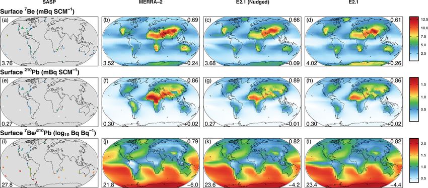
5794                                                                                                  L. T. Murray et al.: GCAP 2.0

Figure 2. Temporal evolution of global mean surface temperature in ◦ C. Each panel from left to right shows the seven future scenarios
arranged by increasing radiative forcing. The black line shows variable tas from the E2.1 ensemble member (r1i1p1f2) that our simulations
are based upon obtained from the ESGF repository. The gray shading represents the annual mean and 2σ spread of all E2.1 ensemble
members archived on ESGF. The red line shows the value from our reruns of r1i1p1f2 to generate the GCAP 2.0 meteorology. The blue line
shows the same but with winds nudged to the MERRA-2 reanalysis. The orange line shows the global mean surface temperature from the
MERRA-2 reanalysis. The horizontal lines show the global pre-industrial climatological mean in our simulations (dotted black) and 1.5 ◦ C
(dashed black) and 2.0 ◦ C (solid black) increases on top of the pre-industrial values.

cal noise associated with the original and repeat simulations’         cipitation rates are forecast to increase in the coming century
different computer architectures (NASA Center for Climate              due to the temperature-driven increase in surface evaporation
Simulations versus the University of Rochester Center for In-          and saturation vapor pressures. Unlike surface air tempera-
tegrated Research Computing). However, tests revealed that             ture, the repeat simulations closely follow the original values
the increased frequency in calls to the radiation code nec-            and are statistically identical except in the recent past histor-
essary to archive hourly radiation fluxes for driving GEOS-            ical simulation, where they are globally higher by 0.9 %. The
Chem explains most of the difference in surface temperature.           MERRA-2 reanalysis shows substantially more interannual
Although almost no locations show significant changes with             variability in its global precipitation rates. Nudging E2.1 de-
respect to local interannual variability (see Fig. S1 in the Sup-      creases the global precipitation rate.
plement), this does lead to a weakly but statistically different          Figures S2 to S51 of the Supplement include detailed
annual mean temperature with respect to the original simu-             comparisons of the seasonal climatologies for all fields in
lation (+0.6 ◦ C for 2001–2014 CE, p value = 0.002). How-              the three meteorology products that may be used to drive
ever, the change is largely a linear offset, with temporal cor-        GEOS-Chem for 2005–2014 CE (MERRA-2, E2.1 nudged
relation remaining high (R = 0.87 for 2001–2014 CE), pro-              to MERRA-2, and the free-running E2.1). In general, most
viding confidence in the ability of GCAP 2.0 to produce                fields show excellent agreement with high pattern (i.e., spa-
changes in composition associated with changes in climate              tial) correlation and small mean difference. However, a few
accurately. Nudging the winds to MERRA-2 reduces this                  fields differ between E2.1 and MERRA-2 that are of interest
offset by influencing the rate of mixing of air between the            for chemical-transport modeling, which we now summarize.
high latitudes and midlatitudes, and the warmer Arctic sur-            The primary difference between MERRA-2 and E2.1 is the
face temperatures in our repeat free-running E2.1 simulations          relative importance of stratiform versus convective precipi-
are in greater agreement with MERRA-2.                                 tation. Whereas both models agree on the total precipitation
   Second, we note that for researchers interested in study-           flux to the surface (Fig. S16), MERRA-2 has a higher rate of
ing a “Paris Agreement”-like future world, in which future             stratiform condensation (Fig. S33) balanced by a higher rate
warming is limited to 2 ◦ C over pre-industrial levels, one            of stratiform re-evaporation (Fig. S45). In contrast, E2.1 has
may use the SSP1-1.9, SSP1-2.6, or SSP4-3.4 scenarios.                 a higher rate of convective condensation (Fig. S34) balanced
However, if one wishes to study a future world with the                by a higher rate of convective re-evaporation (Fig. S44). Fur-
more aggressive goal of limiting warming to 1.5 ◦ C over pre-          thermore, E2.1 has consistently smaller surface roughness
industrial levels, then the only scenario that may be used is          heights over the ocean and vegetated regions than MERRA-
SSP1-1.9.                                                              2; in contrast, MERRA-2 does not appear to include an
   Figure 3 shows the temporal evolution of the global an-             orographic component in its surface roughness calculation
nual mean precipitation rate in the simulations. Global pre-           and therefore has lower surface roughness heights over non-

Geosci. Model Dev., 14, 5789–5823, 2021                                                 https://doi.org/10.5194/gmd-14-5789-2021

L. T. Murray et al.: GCAP 2.0                                                                                                      5795

Figure 3. The same as Fig. 2 but showing the temporal evolution of the global mean precipitation rate in mm d−1 (variable pr on ESGF).

vegetated land surfaces (Fig. S29). Consequently, the E2.1             ulations also lack the relatively large spatial heterogeneity
simulations have lower planetary boundary layer heights                seen in surface winds over the land ice sheets.
over oceans and heavily vegetated regions (globally ∼ 200 m               Figure 5 compares key zonal mean meteorological vari-
lower; Fig. S12) relative to MERRA-2. The E2.1 simula-                 ables generated for GCAP 2.0 with their MERRA-2 coun-
tions also have a lower tropopause pressure by approximately           terparts. Lower- and free-tropospheric air temperatures are
40 hPa (Fig. S23); this has been corrected in version E2.2 of          in agreement between E2.1 and MERRA-2, but the higher
the GCM by moving to a higher vertical resolution (Orbe                tropopause leads to colder temperatures in the upper tro-
et al., 2020b). Lastly, E2.1 has a higher fraction of photosyn-        posphere with respect to MERRA-2. Nudging the winds
thetically active radiation (PAR) present as diffuse (Fig. S10)        removes some of the temperature difference in the extrat-
rather than direct (Fig. S11) radiation, which will promote            ropical upper troposphere but introduces differences in the
higher levels of biogenic emissions (see Sect. 5.2). Note also         free troposphere. Specific humidity agrees between E2.1 and
that MERRA-2 sets PAR fluxes to zero over water. Therefore,            MERRA-2 except for a drier polar free troposphere and
coastal and island cells will underestimate the radiation flux         northern extratropical surface; nudging leads to an additional
in MERRA-2-driven GEOS-Chem simulations, again with                    drying of the stratosphere. The zonal winds agree well be-
consequences for biogenic emissions.                                   tween all simulations, particularly between the MERRA-2
   Figure 4 compares the spatial distribution of key surface           reanalysis and the nudged simulation as to be expected.
meteorological variables generated for GCAP 2.0 with their
MERRA-2 counterparts. Surface air temperature shows near-
perfect agreement in spatial distribution between the E2.1             5     Emissions and boundary conditions
products and MERRA-2. The E2.1 temperatures are slightly
higher than MERRA-2, especially over the Northern Hemi-                This section describes the anthropogenic emission invento-
sphere’s oceans; nudging reduces this difference as previ-             ries and surface boundary conditions from the CMIP6 exper-
ously discussed. Total precipitation in the E2.1 fields has a          iment that have been processed for use by GEOS-Chem, ei-
weaker pattern correlation with MERRA-2 since the free-                ther driven by E2.1 or MERRA-2 meteorology (Sect. 5.1). It
running model produces a split Intertropical Convergence               then evaluates and compares the emission fluxes that are sen-
Zone (ITCZ) in the eastern Pacific (a common issue in free-            sitive to meteorology between MERRA-2 and E2.1-driven
running GCMs; e.g., see Samanta et al., 2019); nudging the             GEOS-Chem simulations in the recent past (Sect. 5.2).
winds corrects the spatial patterns but brings the total precip-
itation rate out of agreement. The surface zonal wind compo-           5.1    Anthropogenic emissions and surface boundary
nent shows excellent agreement in their spatial patterns, al-                 conditions
though the magnitudes are greater in the E2.1 simulations rel-
ative to MERRA-2. The free-running GCM underestimates                  Figure 6 shows the time series of annual mean anthropogenic
the extent of flow towards the Equator over the eastern ocean          emissions and Fig. 7 shows the time series of annual mean
basins, which is corrected in the nudging simulation (and              surface boundary conditions developed for the CMIP6 ex-
may be responsible for the improved ITCZ). The E2.1 sim-               periments and processed for use in GEOS-Chem. Emissions
                                                                       are used for short-lived climate forcers and air pollution
                                                                       precursors. Surface boundary conditions are used to pre-

https://doi.org/10.5194/gmd-14-5789-2021                                                  Geosci. Model Dev., 14, 5789–5823, 2021
5796                                                                                                    L. T. Murray et al.: GCAP 2.0

Figure 4. Comparison of present-day surface meteorology. Columns from left to right show annual climatological means for 2005–2014 CE
in the MERRA-2 reanalysis, our E2.1 simulations with winds nudged to MERRA-2, and our free-running E2.1 simulations. From top to
bottom, rows show surface air temperature in K, total precipitation rate in mm d−1 , the zonal component of the surface wind in m s−1 , and
the meridional component of the surface wind in m s−1 . Gray dots show where the two E2.1 simulations are statistically different from their
MERRA-2 counterparts with respect to interannual variability (p value < 0.05; n = 10 years). The number in the bottom left shows the global
mean value for each panel. The top right number shows the pattern correlation, and the number in the bottom right shows the global mean
difference in the E2.1 simulations with respect to MERRA-2.

scribe long-lived species like chlorofluorocarbons that are             desire (e.g., to use the alternative inventories, regional over-
well mixed in the troposphere but may advect to and re-                 writes and/or scaling factors from the default GEOS-Chem
act within the stratosphere. The emissions and boundary                 configuration).
conditions developed for the CMIP6 experiments include a
historical reconstruction and several future scenarios with             5.1.1    Historical
different target radiative forcings for the end of this cen-
tury. They are hosted on ESGF under the input data sets
                                                                        Historical anthropogenic emissions in CMIP6 are from the
for Model Intercomparison Projects (input4MIPs) project.
                                                                        Community Emissions Data System (CEDS, Hoesly et al.,
They are available from https://esgf-node.llnl.gov/projects/
                                                                        2018). For surface emissions, we processed version 2017-
input4mips (last access: 30 September 2020). These emis-
                                                                        05-18 of the CEDS inventory available at monthly tempo-
sions and boundary conditions have been processed for input
                                                                        ral and 0.5◦ spatial resolution for the eight surface sectors
to GEOS-Chem/GCAP 2.0. They are consistent with those
                                                                        listed in Table 2 and the 1850–2014 CE period. CEDS is
that influenced the climate of the E2.1 simulations used to
                                                                        presently the default global surface anthropogenic emissions
generate the respective GCAP 2.0 meteorology. When users
                                                                        inventory used by GEOS-Chem, although only species for
generate a GCAP 2.0 run directory, the respective CMIP6
                                                                        the full-chemistry simulation have been processed, and these
emissions and boundary conditions for a historical or future
                                                                        emissions are overwritten for many locations by regional in-
scenario are enabled by default. However, users may always
                                                                        ventories. Here, we additionally processed the methane and
modify the Harmonized EMissions COmponent (HEMCO,
                                                                        CO2 fluxes for those GEOS-Chem specialty simulations. All
Keller et al., 2014) configuration to use any emissions they
                                                                        surface emissions increased exponentially over the histor-

Geosci. Model Dev., 14, 5789–5823, 2021                                                   https://doi.org/10.5194/gmd-14-5789-2021
L. T. Murray et al.: GCAP 2.0                                                                                                           5797

Figure 5. Comparison of present-day zonal meteorology. Columns from left to right show annual climatological zonal means for 2005–
2014 CE in the MERRA-2 reanalysis, our E2.1 simulations with winds nudged to MERRA-2, and our free-running E2.1 simulations. From
top to bottom, rows show air temperature in K, specific humidity in kg kg−1 , and the zonal wind component in m s−1 . Gray dots show where
the two E2.1 simulations are statistically different from their MERRA-2 counterparts with respect to interannual variability (p value < 0.05;
n = 10 years).

ical period except for sulfur dioxide (SO2 ), whose emis-                Table 2. CEDS surface emission sectors.
sions peaked in the 1980s (Fig. S52). We also processed
the three-dimensional CEDS aircraft emissions for input into                      Sector   Description
GEOS-Chem as a CMIP6-compliant alternative to the Avia-                           agr      Agriculture (excluding crop burning)
tion Emissions Inventory Code (AEIC, Stettler et al., 2011)                       ene      Energy transformation and extraction
source that is the default in GEOS-Chem. We processed ver-                        ind      Industrial combustion and processes
sion 2017-08-30 of the CEDS aircraft inventory, available                         rco      Residential, commercial, and other
for NO, CO, black and organic carbon, SO2 , and ammonia                           shp      International shipping
(NH3 ) at monthly temporal and 0.5◦ spatial resolution and 25                     slv      Solvents
vertical levels of equal thickness from the surface to 15 km.                     tra      Surface transportation (road; rail; other)
We have vertically regridded to the native 40-level E2.1 res-                     wst      Waste disposal and handling
olution and the reduced stratospheric 47-level MERRA-2
resolution. Global aircraft emissions increased mostly lin-
early across the historical period beginning in approximately            monthly temporal and 0.25◦ spatial resolution. We have re-
1950 CE (Fig. S53).                                                      gridded to 0.5◦ spatial resolution and speciated for input
   In addition, we processed the biomass burning emissions               to GEOS-Chem using a consistent hydrocarbon speciation
from version 1.2 of the Biomass Burning for Model Inter-                 scheme with CEDS. Fire emissions from BB4MIPs increase
comparison Projects (BB4MIPs) inventory (van Marle et al.,               slightly across the historical period. However, interannual
2017). The BB4MIPs reconstruction combines version 4 of                  variability greatly increases in the second half of the 20th
the satellite-based Global Fire Emissions Database (GFED4;               century (Fig. S54), driving the large interannual variabil-
van der Werf et al., 2017, the default biomass burning in-               ity observed in the total emissions during this period (e.g.,
ventory in GEOS-Chem and available since 1997 CE) with                   Fig. 6b).
observational proxies and model simulations from the Fire                   We have prepared version 1.2.0 of the CMIP6 surface
Model Intercomparison Project (FireMIP) for earlier peri-                boundary conditions derived from historical observations
ods. BB4MIPs provides the total mass flux per species at                 (Meinshausen et al., 2017) and available at monthly tempo-

https://doi.org/10.5194/gmd-14-5789-2021                                                     Geosci. Model Dev., 14, 5789–5823, 2021

5798                                                                                                      L. T. Murray et al.: GCAP 2.0

Figure 6. Time series of annual mean CMIP6 anthropogenic emissions for 1850–2100 CE for (a) reactive oxides of nitrogen
(NOx ≡ NO + NO2 ) in Tg N yr−1 , (b) carbon monoxide (CO) in Tg yr−1 , (c) non-methane hydrocarbons (NMHCs) in Tg yr−1 , (d) sul-
fur dioxide (SO2 ) in Tg yr−1 , (e) ammonia (NH3 ) in Tg yr−1 , (f) black carbon (BC) in Tg C yr−1 , and (g) organic carbon (OC) in Tg C yr−1 .
Historical emissions for 1850–2014 CE from Hoesly et al. (2018) are shown as black lines. Future scenarios for 2015–2100 CE from Gid-
den et al. (2019) are shown as colored lines: SSP1-1.9 (green); SSP1-2.6 (blue); SSP4-3.4 (purple); SSP2-4.5 (brown); SSP4-6.0 (orange);
SSP3-7.0 (pink); SSP5-8.5 (red). The shaded blue rectangles indicate periods for which GCAP 2.0 input meteorology is available at the time
of publication.

ral resolution and as 0.5◦ latitude bands. These have been                Table 3. Shared Socioeconomic Pathway (SSP) narratives.
regridded to 0.5◦ global spatial resolution for input into
GEOS-Chem. Carbon dioxide, methane, and nitrous oxide                          SSP1     Sustainability – taking the green road
have monotonically increased since the pre-industrial era due                  SSP2     Middle of the road
to anthropogenic activity, whereas shorter-lived stratospheric                 SSP3     Regional rivalry – a rocky road
ozone-depleting substances peaked around the turn of the                       SSP4     Inequality – a road divided
last century following their ban under the Montreal Protocol                   SSP5     Fossil-fueled development – taking the highway
(Fig. 7).

5.1.2   Future scenarios                                                  society would achieve the target radiative forcing. SSP1 as-
                                                                          sumes low challenges to mitigation and adaptation (van Vu-
The future anthropogenic emissions and boundary conditions                uren et al., 2017), SSP2 assumes medium challenges to mit-
used by CMIP6 and processed here for GCAP 2.0 are sum-                    igation and adaptation (Fricko et al., 2017), SSP3 assumes
marized by Riahi et al. (2017). In brief, the so-named Shared             high challenges to mitigation and adaptation (Fujimori et al.,
Socioeconomic Pathways (SSPs) are determined from inte-                   2017), SSP4 assumes low challenges to mitigation and high
grated assessment modeling (IAM) of five future societal                  challenges to adaptation (Calvin et al., 2017), and SSP5 as-
narratives that may be followed to limit future warming to                sumes high challenges to mitigation and low challenges to
a target radiative forcing. The nomenclature for character-               adaptation (Kriegler et al., 2017).
izing the SSP scenarios is SSPx-y.z (or SSPxyz), where x                     For GCAP 2.0, we focus on seven scenarios correspond-
is the number of the future narrative (1 to 5; Table 3), and              ing to Tiers 1 and 2 of the ScenarioMIP experiment: SSP1-
y.z represents the target radiative forcing in W m−2 at the               1.9, SSP1-2.6, SSP4-3.4, SSP2-4.5, SSP4-6.0, SSP3-7.0, and
end of the 21st century ranging from 1.9 (extreme mitiga-                 SSP5-8.5 (O’Neill et al., 2016). Assumptions about future
tion; low warming) to 8.5 (low mitigation; extreme warm-                  population growth, urbanization, gross domestic production
ing). The names of the five narratives are listed in Table 3,             (GDP), energy, land use, and air pollution trends of the SSP
and each employs different assumptions about how global                   IAM scenarios are described in a series of papers (Cre-

Geosci. Model Dev., 14, 5789–5823, 2021                                                     https://doi.org/10.5194/gmd-14-5789-2021
L. T. Murray et al.: GCAP 2.0 5799
Figure 7. Time series of annual mean CMIP6 surface boundary conditions for 1850–2100 CE. Individual panels show the temporal evo-
lution of (a) carbon dioxide (CO2 ) in ppmv (≡ µmol mol−1 ), (b) methane (CH4 ) in ppbv (≡ nmol mol−1 ), (c) total chlorofluorocarbons
(CFCs ≡ CFC11 + CFC12 + CFC113 + CFC114 + CFC115) in pptv (≡ pmol mol−1 ), (d) nitrous oxide (N2 O) in pptv, (e) methyl chlo-
ride (CH3 Cl) in pptv, (f) total hydrochlorofluorocarbons (HCFCs ≡ HCFC141b + HCFC142b + HCFC22) in pptv, (g) methyl chloroform
(CH3 CCl3 ) in pptv, (h) carbon tetrachloride (CCl4 ) in pptv, (i) dichloromethane (CH2 Cl2 ) in pptv, (j) chloroform (CHCl3 ) in pptv, (k) methyl
bromide (CH3 Br) in pptv, and (l) total halons (≡ Halon1211 + Halon1301 + Halon2402) in pptv. Historical boundary conditions are from
Meinshausen et al. (2017) and future boundary conditions are described by Riahi et al. (2017). The shaded blue rectangles indicate periods
for which GCAP 2.0 input meteorology is available at the time of publication.
spo Cuaresma, 2017; Dellink et al., 2017; Jiang and O’Neill, rative assumptions strongly influence the global and regional
2017; Leimbach et al., 2017; Samir and Lutz, 2017; Bauer emission changes. Furthermore, we note that the historical
et al., 2017; Popp et al., 2017; Rao et al., 2017). Version emissions inventories have large amounts of interannual vari-
1.1 of these scenarios (Gidden et al., 2019) was obtained ability (primarily due to biomass burning), whereas the SSP
from input4MIPs on ESGF and available at 0.5◦ spatial and scenarios have very low interannual variability. This high-
monthly resolution for 2015 CE and then every 10 years be- lights the necessity for CTM studies such as those that may
ginning with 2020 CE and ending with 2100 CE. These fu- be accomplished by GCAP 2.0 that can explore the impact
ture emissions were processed for input to GEOS-Chem in of a wider range of future emission trajectories on air quality,
the same way as the historical emissions and boundary con- short-lived climate forces, and stratospheric ozone in future
ditions. Linear interpolation was used to develop individual warmer climates whose meteorology is primarily driven by
yearly emissions between the available decadal values. In ad- changes in CO2 . It also highlights the necessity for perform-
dition to the sectors of Table 2, future CO2 emissions include ing simulations long enough to establish robust statistics for
a “neg” sector that considers negative emission (i.e., carbon chemistry–climate interactions (e.g., Garcia-Menendez et al.,
capture). 2017).
From the perspective of the simulated climate, the forcing
that dominates the end-of-the-century response is the CO2 5.2 Natural emissions
abundance. Therefore, CO2 is the only gas that monoton-
ically increases with future forcing target values (Fig. 7a). Figure 8 shows the climatological mean emission fluxes for
The trajectories of the remainder of the well-mixed green- key species whose emissions are sensitive to meteorology.
house gases, stratospheric ozone-depleting substances, short- Figures S55–S60 in the Supplement provide seasonal details
lived climate forcers, and air-pollution precursors vary be- for each species.
tween the SSP scenarios and target forcings (Figs. 6 and 7b– Emission fluxes sensitive to meteorology and thereby grid
l). For example, methane in 2100 CE is highest in the SSP3- resolution began to be pre-processed offline at high spatial
7.0 scenario, not SSP5-8.5 (Fig. 7b). Because ammonia is resolution in version 12.4.0 of GEOS-Chem. This was to fa-
primarily produced from agriculture and the world popula- cilitate the calculation of consistent emissions between the
tion will continue to grow, it is the only emission expected to various cubed-sphere geometries of the GCHP variant of the
remain constant or grow into the future. Otherwise, the nar- model (Eastham et al., 2018, see Sect. 3.2), although the
option to calculate these emissions online was maintained
https://doi.org/10.5194/gmd-14-5789-2021 Geosci. Model Dev., 14, 5789–5823, 20215800 L. T. Murray et al.: GCAP 2.0 Figure 8. Annual mean spatial distribution of meteorology-dependent emission fluxes for 2005–2014 CE. Each column from left to right shows emission fluxes calculated using: MERRA-2 meteorology, E2.1 meteorology nudged to MERRA-2, and the free-running E2.1 meteorology, respectively. Each row from top to bottom shows emission fluxes for: (a–c) isoprene (2-methyl-1,3-butadiene; CH2 =C(CH3 )CH=CH2 ) from terrestrial plants in 10−9 kg m−2 s−1 , (d–f) dimethylsulfide ((CH3 )2 S; DMS) from marine organisms, (g– i) aeolian mineral dust, (j–l) aeolian sea salt, (m–o) the vertically integrated source of NO from lightning, and (p–r) NO from soil mi- crobial activity, respectively. Gray dots indicate locations where the two E2.1-driven simulations show statistically significant differences (p value < 0.05; n = 10 years) with respect to the MERRA-2-driven simulation. The value in the lower left of each panel gives the globally integrated source in (a–l) Tg yr−1 or (m–r) Tg N yr−1 . The number in the lower (upper) right of each panel gives the total difference (pattern correlation) of the E2.1-driven simulations with respect to their respective MERRA-2-driven values. through online extensions in the HEMCO processing code dalone” version of HEMCO with a HEMCO_Config.rc file (Keller et al., 2014). The default behavior for GCAP 2.0 is to from a GCClassic version of GCAP 2.0. Here, we compare use online calculations to respond to the underlying climate. the online emission fluxes in our MERRA-2-driven simula- Users who wish to run GCHP with GCAP 2.0 may quickly tion to those of our E2.1-driven simulations. pre-process offline natural emission fluxes using the “stan- Geosci. Model Dev., 14, 5789–5823, 2021 https://doi.org/10.5194/gmd-14-5789-2021
L. T. Murray et al.: GCAP 2.0                                                                                              5801

   Panels a–c of Fig. 8 show the spatial distribution of iso-    olution for input as a meteorological parameter to GEOS-
prene from terrestrial plants. Emissions of non-methane hy-      Chem (see Sect. 4). Both lightning flash density calculations
drocarbons (NMHCs) from terrestrial plants follow version        are ultimately based on the same cloud-top height scheme
2.1 of the Model of Emissions from Gases and Aerosols from       of Price and Rind (1992) and global mean lightning flash
Nature (MEGAN), which responds positively to changes in          rates are tuned to climatology in the recent past (Cecil et al.,
diffuse photosynthetically active radiation (PAR), recent sur-   2014). However, because the spatial and seasonal climatol-
face air temperature, and soil root wetness (Guenther et al.,    ogy in the MERRA-2-driven simulations is constrained by
2012). There is an option for emissions to respond to CO2        satellite observations (Murray et al., 2012), which is not ap-
abundance as well (Tai et al., 2013). Because E2.1 has a         propriate for a free-running GCM, the spatial patterns differ
greater proportion of PAR present as diffuse radiation, iso-     between the simulations. Therefore, E2.1 overestimates the
prene emissions in E2.1-driven simulations are about 40 %        fraction of lightning in the tropics with respect to the extrat-
higher than in the MERRA-2-driven simulation.                    ropics and puts too much lightning over South America and
   Panels d–f of Fig. 8 show a very tight agreement in the       Oceania and not enough over Africa. It is also worth empha-
spatial pattern and magnitude of the flux of dimethylsulfide     sizing that we do not know how lightning has changed since
(DMS; (CH3 )2 S) produced by marine phytoplankton. Emis-         the pre-industrial era or will change in a warming world (e.g.,
sions of NMHCs from marine environments are represented          Williams, 2005; Price, 2013; Murray, 2016, 2018; Finney
as the product of prescribed seawater concentration distri-      et al., 2018).
butions and sea-to-air transfer velocities calculated via the       Panels p–r of Fig. 8 show the source of NO from soil mi-
parameterization of Nightingale et al. (2000a, b). The latter    crobial activity. The parameterization is described by Hud-
respond to sea-surface temperatures and surface wind veloc-      man et al. (2012) and responds to surface air temperature,
ities.                                                           wind speed, soil wetness, cloud fraction, downwelling short-
   Panels g–i of Fig. 8 compare the source of mineral dust be-   wave radiation, and snow/ice cover. To a lesser degree, light-
tween the simulations. We use the Dust Entrainment and De-       ning can also influence the soil NO source through its impact
position (DEAD) scheme for mineral dust evasion (Zender          on nitrate deposition to the soils. The spatial correlation is
et al., 2003), which responds to changes in surface friction     excellent between the different sources, although the E2.1
velocity (u∗ ), roughness height, snow/ice cover and depth,      magnitude is higher by about 40 %.
soil wetness, pressure, specific humidity, and temperature.         Lastly, we note the important and variable geologic source
Dust mobilization was found in our tests to be extremely         of SO2 . Volcanic emissions of SO2 in GEOS-Chem are nor-
sensitive to the meteorology product used, with poor spatial     mally prescribed from the Aerosol Comparisons between
correlation (R ≤ 0.26) and with each meteorology product         Observations and Models (AeroCom) point-source inventory
yielding a different order of magnitude in its global total.     (Carn et al., 2015), with data available since 1978 CE. The
Therefore, we have determined respective scaling factors for     CMIP6 experiment did not provide historical or future emis-
the E2.1 simulations that bring the present-day global total     sion fluxes for volcanism. Instead, input4MIPs provided time
into agreement with the MERRA-2-driven value. These are          series of stratospheric aerosol surface area densities and ef-
included by default in the GCAP 2.0 run directories for the      fective radii with which to force the GCMs. Therefore, when
DEAD dust scheme.                                                users generate a GCAP 2.0 run directory, they are given the
   Panels j–l of Fig. 8 show the source of sea-salt aerosol.     option to select a fixed historical AeroCom year from which
The sea-salt mobilization scheme is described by Jaeglé et al.   to prescribe their volcanic emissions.
(2011) and responds to sea-surface temperature, surface wind
velocity, and the fraction of sea-ice coverage. There is an
excellent agreement between each source’s spatial distribu-      6   Model evaluation
tions, although the stronger surface winds in E2.1 lead to
15 %–20 % higher emissions in the E2.1 simulations, espe-        This section evaluates the performance of GCAP 2.0 driven
cially over the Southern Ocean.                                  by E.21 versus MERRA-2 meteorology for the recent past
   Panels m–o of Fig. 8 show the column-integrated source        through comparison with observations. We first evaluate
of NO from lightning. In MERRA-2, lightning flash densities      model physics and transport using the “TransportTracers”
(flashes km−2 s−1 ) are pre-calculated offline from MERRA-       variant of GEOS-Chem (Sect. 6.1). We then evaluate the
2 convective cloud depths at 0.5◦ latitude by 0.625◦ longitude   standard full-chemistry mechanism (Sect. 6.2).
spatial and 3 h temporal resolution. These densities are then       All simulations were performed at 4◦ latitude by 5◦ lon-
input as a meteorological parameter to GEOS-Chem, from           gitude horizontal resolution for the period 2001–2014 CE,
which vertical profiles of NO production are determined fol-     with meteorology respectively prescribed from MERRA-2,
lowing Murray et al. (2012). For the GCAP 2.0 meteorology,       E2.1 nudged to MERRA-2, and the free-running E2.1 simu-
flash rates are calculated online in the E2.1 moist convec-      lation. All simulations used version 12.9.3 of GEOS-Chem
tion code following the description in Kelley et al. (2020)      (https://doi.org/10.5281/zenodo.3974569, The International
and archived at E2.1 native spatial and hourly temporal res-     GEOS-Chem User Community, 2020) with modifications as

https://doi.org/10.5194/gmd-14-5789-2021                                           Geosci. Model Dev., 14, 5789–5823, 2021
5802                                                                                              L. T. Murray et al.: GCAP 2.0

described throughout the paper. The E2.1 meteorology fields         lower stratosphere (Lal et al., 1958). The source of 7 Be is
were regridded from their native resolution upon input to           updated for this work to use the parameterization of Usoskin
GEOS-Chem by FlexGrid. The E2.1 simulations used the na-            and Kovaltsov (2008). Mean solar activity is assumed (so-
tive 40-layer resolution and the MERRA-2 simulations used           lar modulation potential 8 = 670 MV), leading to an average
the 47-layer reduced-stratospheric resolution (see Fig. 1).         production rate of 0.065 atoms cm−2 s−1 ; about 60 % in the
Identical initial conditions were regridded to each model’s         stratosphere and 40 % in the troposphere. Like 210 Pb, 7 Be
respective vertical resolution. The first 4 years of each simu-     is rapidly taken up by submicron aerosol particles (Bondi-
lation were discarded as initialization, with the remaining 10      etti et al., 1988; Maenhaut et al., 1979; Papastefanou, 2009;
years used for evaluation and statistics. All prescribed emis-      Papastefanou and Ioannidou, 1996; Sanak et al., 1981). It
sions were identical between each simulation.                       is subsequently transported until removal by deposition or
                                                                    radioactive decay (half-life of 53.3 d). 7 Be has been used
6.1    Transport                                                    to constrain vertical transport, wet deposition fluxes, and
                                                                    stratosphere–troposphere exchange in models (e.g., Allen
Model transport and physical processes may be evaluated             et al., 2003; Brost et al., 1991; Koch et al., 1996; Liu et al.,
against observations using the “TransportTracers” variant of        2001, 2016; Barrett et al., 2012).
GEOS-Chem. We focus on four tracers of particular util-                Table 4 gives the atmospheric budget of the three radionu-
ity: sulfur hexafluoride (SF6 ), radon-222 (222 Rn), lead-210       clides driven by the three meteorological products.
(210 Pb), and beryllium-7 (7 Be).
   Sulfur hexafluoride is a trace gas of anthropogenic origin       6.1.1   Horizontal mixing
that is chemically and physically inert on human timescales
(lifetime of 3200 years). It is primarily emitted at the sur-       Figure 9 shows observed meridional and vertical gradients of
face in the Northern Hemisphere (Maiss and Brenninkmeijer,          SF6 with respect to Cape Matatula, American Samoa (SMO),
1998). Its meridional gradient may be used to test the rate         in the remote tropical southern Pacific. The observations
of interhemispheric mixing (Rigby et al., 2010; Hall et al.,        are version 2.1.1 of the NOAA Carbon Cycle Group SF6
2011) and its vertical gradients may be used to infer the age       ObsPack (https://doi.org/10.25925/20180817, NOAA Car-
of air in the stratosphere (Waugh and Hall, 2002; Waugh,            bon Cycle Group ObsPack Team, 2018) and represent a
2009). Its meridional gradients may also be used to infer the       mixture of surface in situ, flask, tower, and aircraft sources
tropospheric age of air (Waugh et al., 2013). Here, we use          from 2005–2014 CE. Observations were aggregated at model
emissions from version 4.2 of the Emissions Database for            spatial and monthly temporal resolution, compared to that
Global Atmospheric Research (EDGAR), available at 0.1◦              month’s SMO value, from which zonal climatologies were
global resolution for 1970–2008.                                    determined. Also shown is the value of each simulation
   Terrigenic 222 Rn is an inert, insoluble, short-lived (half-     sampled and processed as in the observations. In all sim-
life of 3.8 d) noble gas produced from the slow decay of            ulations, GEOS-Chem underestimates the cross-equatorial
226 Ra (half-life of 1600 years) found in uranium ores. Its         meridional gradient by 17 %–26 %, an improvement over
evasion from surface soils is relatively uniform and constant       GEOS-Chem driven by earlier meteorology products (see
and is as described by Jacob et al. (1997). Its insolubility        Supplement of Murray et al., 2014). However, this suggests
and timescale of decay make it a useful tracer for diagnos-         that the interhemispheric mixing rate in the model is too fast
ing quick vertical mixing within atmospheric models from            and/or that the EDGAR inventory underestimates the emis-
boundary layer processes and moist convection (e.g., Allen          sion growth rate in the Northern Hemisphere relative to the
et al., 1996; Brost and Chatfield, 1989; Considine et al.,          Southern Hemisphere. Meanwhile, meridional mixing rates
2005; Feichter and Crutzen, 1990; Hauglustaine et al., 2004;        in the Southern Hemisphere are consistent with the obser-
Jacob and Prather, 1990; Jacob et al., 1997; Lambert et al.,        vations in all simulations. The E2.1 simulation slightly bet-
1982; Mahowald et al., 1995; Stockwell et al., 1998).               ter matches the cross-equatorial gradient than the MERRA-2
   Radiogenic 210 Pb is the chemically inert decay product of       and nudged simulations, but E2.1 greatly underestimates the
222 Rn. It is readily taken up by submicron aerosol particles       lower stratospheric gradient (see Sect. 6.1.3).
and subsequently removed from the atmosphere by deposi-
tion or decay (Bondietti et al., 1988; Maenhaut et al., 1979;       6.1.2   Vertical mixing – troposphere
Preiss et al., 1996; Sanak et al., 1981). Because of its rela-
tively long lifetime (half-life of 22.2 years), nearly all 210 Pb   We assess vertical mixing within the troposphere using verti-
is removed via deposition. As its source from 222 Rn is rela-       cal profiles of 222 Rn and the ratio of 7 Be to 210 Pb in surface
tively well known, and there is a global and long-term sur-         air.
face deposition flux inventory (Preiss et al., 1996), it is the        Figure 10 shows simulated climatological 222 Rn profiles
standard test for model deposition.                                 sampled at the month and location of the available obser-
   Cosmogenic 7 Be is produced by cosmic-ray spallation of          vations, also plotted. Observations are scarce and available
N2 and O2 , predominantly in the polar upper troposphere and        only at northern extratropical continental locations (Bradley

Geosci. Model Dev., 14, 5789–5823, 2021                                              https://doi.org/10.5194/gmd-14-5789-2021
You can also read