Particle capture by drops in turbulent flow
←
→
Page content transcription
If your browser does not render page correctly, please read the page content below
Particle capture by drops in turbulent flow

                                                                       A. Hajisharifi
                                                        Department of Engineering and Architecture,
                                                           University of Udine, 33100 Udine, Italy
arXiv:2011.02228v1 [physics.flu-dyn] 4 Nov 2020

                                                                       C. Marchioli∗
                                                        Department of Engineering and Architecture,
                                                        University of Udine, 33100 Udine, Italy and
                                                  Department of Fluid Mechanics, CISM, 33100 Udine, Italy

                                                                         A. Soldati
                                                       Institute of Fluid Mechanics and Heat Transfer,
                                                             TU Wien, 1040 Wien, Austria and
                                                        Department of Engineering and Architecture,
                                                           University of Udine, 33100 Udine, Italy
                                                                  (Dated: November 5, 2020)

                                                                            1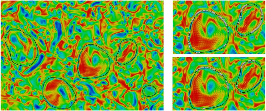
Abstract
    ABSTRACT
We examine the process of particle capture by large deformable drops in turbulent
channel flow.     We simulate the solid-liquid-liquid three-phase flow with an Eulerian-
Lagrangian method based on Direct Numerical Simulation of turbulence coupled with
a Phase Field Model, to capture the interface dynamics, and Lagrangian tracking of small
(sub-Kolmogorov) particles. Drops have same density and viscosity of the carrier liquid,
and neutrally-buoyant solid particles are one-way coupled with the other phases. Our
results show that particles are transported towards the interface by jet-like turbulent mo-
tions and, once close enough, are captured by interfacial forces in regions of positive surface
velocity divergence. These regions appear to be well correlated with high-enstrophy flow
topologies that contribute to enstrophy production via vortex compression or stretching.
Examining the turbulent mechanisms that bring particles to the interface, we have been
able to derive a simple mechanistic model for particle capture. The model can predict the
overall capture efficiency and is based on a single turbulent transport equation in which
the only parameter scales with the turbulent kinetic energy of the fluid measured in the
vicinity of the drop interface. The model is valid in the limit of non-interacting particles
and its predictions agree remarkably well with numerical results.

∗
    Corresponding Author: marchioli@uniud.it

                                               2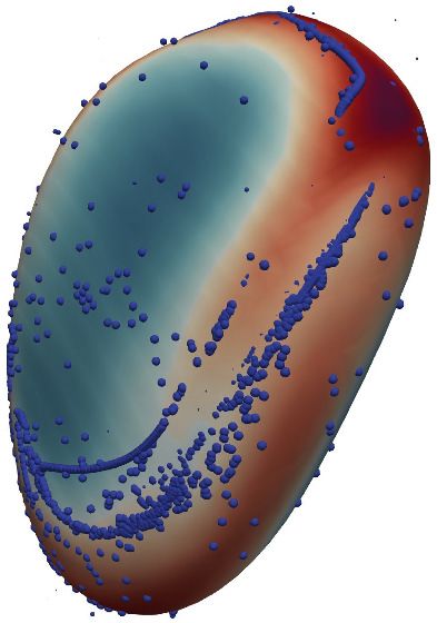
I.    INTRODUCTION

     The process of particle capture by drops or bubbles in a turbulent flow is of rel-
evance in a number of industrial applications requiring particulate abatement, e.g.
via wet scrubbing [1–3]. The very same process is also observed in environmental
problems, such as accidental oil spills in which oil interacts with sediments to form
oil-particle aggregates that may affect the transport of spilled oil and enhance oil
biodegradation [4]. In these applications, particle capture occurs in two steps: First,
particles move towards the drop/bubble surface under the influence of turbulence
in the carrier liquid, possibly aided by external forces as in the case of electro-
static scrubbing [5, 6]; then particles stick the drop/bubble surface upon inertial
impaction or turbulent diffusion. Particle behaviour upon impaction determines the
overall attachment efficiency, which in turn affects the overall capture efficiency of
the drop/bubble. In this context, a crucial physical property is surface tension,
which controls drop/bubble deformability, drives particle adhesion and leads to the
formation of a layer that may change the mechanical and mass transport properties
of the interface [7–9].
     Aim of the present study is to elucidate the physical mechanisms that govern
particle capture at the surface of a swarm of deformable drops transported by a
turbulent flow, focusing in particular on the characterization of the flow events that
bring particles to the surface. This interest is motivated by the need of detailed
information about the near-interface flow field in usual engineering practice, e.g. for
the development of physics-based models or correlations able to predict transfer rates
across a liquid-liquid interface [10]. Currently, industrial CFD tools can only rely on
mechanistic correlations to predict the capture efficiency of a full-scale equipment
[10, 11].
     To study the targeted three-phase turbulent flow, we use a computational ap-
proach that couples for the first time the direct numerical simulation (DNS) of the
carrier fluid and drops with an interface-capturing method for the evolution of the
drop surface and a Lagrangian tracking method for the particle dynamics.
     Three-phase computational models like the one adopted here pose computational
challenges in terms of modelling the interactions among the different phases and
the complex dynamics produced by a moving, deformable interface [12]. drops in-

                                           3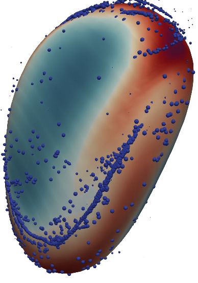
troduce additional physical mechanisms into the flow due to their ability to deform
but also to breakup and coalesce with other drops, thus changing the overall surface
area available for particle capture. The problem is complicated further by the wide
range of length scales involved, from the interface thickness - O(10−9 ) m - to the
particle size - O(10−5 ) m - to the drop size - O(10−2 ) m. Because of these complex-
ities, most of the numerical studies available in the literature focus on the role that
surface physicochemical forces have in determining particle adsorption in no-flow or
viscous flow conditions, when particle-drop interactions are not affected by the flow
hydrodynamics. Examples include the study of the behaviour of a single particle
trapped at a planar fluid interface [13, 14], the surface stress tensor modification
for a pendant drop covered by a monolayer of particles in the low-Reynolds-number
limit [15], or the attachment of a colloidal particle to the surface of an immersed
bubble rising in still fluid [16], to name a few recent works. Also relevant is the study
by [17], who developed a DEM-VOF method to reproduce drop formation and in-
terface perturbations from a single particle. The same methodology was applied by
[18] to study gas-solid-liquid-flows of relevance for sedimentation problems.
  All of the above-mentioned studies have contributed to the physical understand-
ing of particle-laden fluid interfaces, but do not consider turbulent flow conditions:
Clearly, the flow hydrodynamics must be accounted for in turbulent systems, which
are the focus of our investigation and (to the best of our knowledge) have not
been examined before. Intuitively, one expects particles to be brought in the near-
interface region by coherent jet-like fluid motions able to generate local deformations
of the drop surface along the surface itself (via the tangential stress they generate)
but also along the interface-normal direction (via the pressure fluctuations and nor-
mal stresses they induce). When strong enough, these deformations will produce a
change in the topology of the flow surrounding each drop, as compared to the topol-
ogy of an unladen flow [19], and will play a role in the particle adhesion process. To
examine this role, we have concentrated our analysis on the fluid motions that occur
in the proximity of the interface, where the smallest hydrodynamic length scales are
typically located. For this purpose, we consider a density-/viscosity-matched flow
that allows uncoupling of inertial effects associated with particle size from those due
to differential density [20]: Even in this simplified case, the presence of an interface
is crucial as it represents an elastic, compliant boundary that can modulate the

                                          4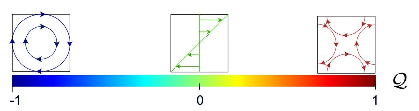
overall energy and momentum transfer the carrier phase and the drops [21].
  The paper is structured as follows. In Sec. II, the physical problem and the
numerical methodology are presented: Specifically, we investigate the interaction
between sub-Kolmogorov particles and super-Kolmogorov drops in a channel flow
configuration, considering particles with low, albeit different, inertia. In Sec. III,
first we characterize the flow topology near the locations of the interface at which
particles get captured, by means of classical topology indicators [22].
  Then, we examine the time evolution of the fraction of captured particles, propos-
ing a simple predictive model to estimate the capture rate. Finally, in Sec. V the
main findings are summarized and future perspectives are provided.

II.    PHYSICAL PROBLEM AND METHODOLOGY

  The physical problem considered in this study consists of turbulent three-phase
channel flow in which large, deformable drops and small, spherical particles are
transported by a carrier liquid. To numerically simulate this flow, we performed
Direct Numerical Simulation (DNS) of the Navier-Stokes equations to provide an
accurate representation of turbulence, using a Phase-Field Method (PFM) to de-
scribe the dynamics of the drop surface (referred to as interface hereinafter) via the
Cahn-Hilliard equations and a Lagrangian approach based on a suitably-simplified
version of the Maxey-Riley-Gatignol equation to compute the trajectory of the par-
ticles. Note that the Navier-Stokes equations, which define the hydrodynamics of
the system, include an additional force term to account for the presence of the inter-
face. In the following, the PFM is presented first and then the force coupling with
the Navier-Stokes equations is described. Finally, the Lagrangian particle tracking
is discussed.

  A.    Modeling of the interface dynamics

  The phase field method adopted in this study uses a scalar field (order parameter)
to describe the transport of the phase field φ, which provides the instantaneous
shape and position of the interface. The phase field is constant in the bulk of both
the carrier phase (φ = −1) and the drops (φ = −1), while undergoing a smooth

                                         5
transition across the interfacial layer. The position of the interface is given by the
iso-level φ = 0. The time evolution of the order parameter φ is given by the Cahn-
Hilliard equation, which reads in dimensionless form as
∂φ 1
+ u · ∇φ = ∇ 2 µφ + f p , (1)
∂t P eφ
where u = (u, v, w) is the carrier fluid velocity field vector, P eφ is the Péclet num-
ber (ratio between the diffusive and convective time scale controlling the interface
relaxation), µφ is the chemical potential and fp is a penalty flux (not accounted for
in the standard phase field formulation) introduced to force the interface toward its
equilibrium by reducing the diffusive fluxes induced by the gradient of the chemical
potential µφ [23–25]: Through this term, the equilibrium interfacial profile can be
maintained and the drawbacks of the standard formulation (e.g. mass leakage) can
be overcome. The penalty flux is defined as:
λ 2 1 2 ∇φ
fp = ∇ φ− √ ∇ · (1 − φ ) , (2)
P eφ 2Ch |∇φ|
with the parameter λ set according to the scaling proposed by [24, 25]. The chem-
ical potential µφ is defined as the variational derivative of the Ginzburg-Landau free
energy functional, F[φ, ∇φ]. The functional composed as the sum of two different
contributions:
Z
F[φ, ∇φ] = (f0 + fm ) dΩ , (3)
Ω
where Ω is the reference domain. The two contributions are defined as follows
[26, 27]
1
f0 = (φ − 1)2 (φ + 1)2 . (4)
4
Ch2
fm = |∇φ|2 . (5)
2
The terms f0 and fm are the functions of phase field φ. The former, f0 , is the
double well potential that describes the tendency of the system to separate into two
pure fluids and is defined and the latter, fm , is the mixing energy and accounts for
6the energy stored at the interface (i.e. the surface tension); Ch is the Cahn num-
ber, representing the dimensionless thickness of the interfacial layer. The chemical
potential is thus obtained as
F[φ, ∇φ]
µφ = = φ3 − φ − Ch2 ∇2 φ . (6)
δφ
When the system is at equilibrium, the chemical potential is uniform over the
entire domain. The equilibrium profile for a flat interface located at s = 0, s being
the coordinate normal to the interface, can be obtained by solving ∇µφ = 0, which
yields the following hyperbolic tangent profile
s
φeq (s) = tanh √ , (7)
2Ch
which ensures a smooth transition between the limiting values φ = ±1 that are
reached in the bulk of each phase.
B. Hydrodynamics
The hydrodynamics of the three-phase flow is described by the Continuity and
Navier-Stokes equations, which is coupled with the Cahn-Hilliard equation previ-
ously introduced. This computational model can handle non-matched properties in
general cases [27, 28]; density and viscosity can be defined as a function of the phase
field φ, but In this study we assume that the two Eulerian phase, namely the carrier
fluid (denoted by subscript f ) and the drops (denoted by subscript d), have matched
density (ρ = ρf = ρd ) and matched viscosity (η = ηf = ηd ). According to this one-
fluid formulation, the dimensionless Continuity and Navier-Stokes equations read
as
∇·u=0 , (8)
∂u 1 Ch 3
+ u · ∇u = −∇p + ∇2 u + √ ∇ · τc , (9)
∂t Reτ We 8
where ∇p is the pressure gradient, which includes both the mean pressure gradient
that drives the flow and the fluctuating part; Reτ = uτ h/νf is the friction Reynolds
p
number (based on the friction velocity uτ = τw /ρf , with τw the mean wall shear
7stress, the channel half height h and the fluid kinematic viscosity νf );W e = ρf u2τ h/σ
is the Weber number, based on the surface tension σ of a clean interface; τc =
|∇φ|2 I − ∇φ ⊗ ∇φ is the Korteweg stress tensor, which accounts for the interfacial
force induced on the flow by the occurrence of capillary phenomena due to non-local
molecular interactions at the interface on the two immiscible liquid phases.
C. Lagrangian tracking and particle-interface interaction model
The motion of the particles is described by a set of ordinary differential equations
for the particle velocity and position, which stem from the balance of the forces
acting on the particles, which are assumed to be neutrally-buoyant (ρp = ρf , no
effect of gravity) and smaller in size than the Kolmogorov length scale. In this
study, we considered two force contributions: The drag force and the capillary force
that is exerted on the particles when they interact with the interface, thus allowing
for particle adhesion. With the above assumptions the Lagrangian equations of
motion for the particles, in dimensionless vector form, read as
∂xp
= up , (10)
dt
∂up u@p − up 6A Reτ D
= (1 + 0.15Rep0.687 ) + , (11)
∂t | St {z W e dp 3
} |ρp /ρf {z }
Drag force
Capillary force
where xp and up are the particle position and velocity, respectively; u@p is the
fluid velocity at particle position (obtained using a sixth-order Lagrange polynomials
interpolation scheme); St = τp /τf is the Stokes number, ratio of the particle relax-
ation time τp = ρp d2p /18µf (with dp the particle diameter and µf the fluid dynamic
viscosity) to the carrier fluid characteristic time τf = νf /uτ 2 ; Rep = |u@p −up |dp /νf
is the particle Reynolds number, introduced to correct the drag coefficient using the
Schiller-Naumann correlation [29] and D is the interaction distance between the
center of mass of the particle and the nearest zero-level point on the fluid interface,
which defines the range of action of the capillary force. The expression of the capil-
lary force in Eq. (11) corresponds to the case of small spherical particles adsorbed at
a fluid interface, and has been adopted in several previous studies to model particle
8particle-interface interactions [15, 18, 30]. Specifically, the dimensional expression
of the force reads as
AπσDn
if D ≤ dp
Fc = (12)
0 if D > dp
where A is a dimensionless parameter that characterises the magnitude of the
capillary adhesion force (which incorporates the effect of the contact angle θ between
the particle and the interface as well as the effect of the particle-to-drop size ratio)
and n is the normal unit vector pointing from the particle center of mass to the zero-
level set of φ. From Eq. (12), it is clear that Fc reproduces the effect of a potential
well centered at the interface that favours particle adhesion and attachment to the
surface of the drop as soon as the particle touches the interface. Albeit based on
a mechanistic (rather than phsyics-based) model of the capillary force, Eq. (12)
represents the state of the art as far as particle-interaction models are concerned
[15].
The value of the parameter A is chosen to satisfy the condition that the adsorption
energy Eads = πσr2 (1−| cos θ|)2 , corresponding to the difference between the energy
of a particle fully displaced from the interface into the bulk phase and the energy of
the particle settling at equilibrium at the interface, balances the desorption energy
Edes = 21 Aπσr2 , corresponding to the energy required for particle detachment from
the interface [30, 31]. Note that the expressions for Eads and Edes are exact for an
isolated, chemically homogeneous spherical particle on a flat surface [31]. Assuming
a contact angle θ = 90o , this balance yields A = 2, which is the value used in our
simulations. Additional runs for different values of A (specifically: A = 0.01 and
0.1) were also performed to assess the effect of a change in the magnitude of Fc on
the capture process. As far as the statistical quantities discussed in Sec. III are
concerned, no major effect was observed (small quantitative modifications).
We remark that, in this study, only particles with tiny inertia are considered.
For these particles, the capillary force is expected to be dominant over the other
hydrodynamic forces (drag, in particular) in close proximity of the interface, thus
favoring particle adhesion. However, this process may be significantly affected by
the turbulence in the bulk of the carrier fluid, which tends to deform continuously
the interface and modify the topology of the flow structures with which the particles
9interact as they approach the drop. Our aim is precisely to highlight the role played
by these local flow structures and quantify their effect on particle adhesion.
D. Numerical method
The governing equations (1), (8) and (9) are solved numerically using a pseudo-
spectral method that transforms the field variables into wave space. Specifically,
Fourier series are used to discrete the variables in the homogeneous directions
(streamwise x and spanwise y), while Chebychev polynomials are used in the wall-
normal direction, z. The Helmholtz-type equations so obtained are advanced in
time using an implicit Crank-Nicolson scheme for the linear diffusive terms and an
explicit two-step Adams-Bashforth scheme for the non-linear terms. Time-wise, the
Cahn-Hilliard equation is discretized using an implicit Euler scheme, which allows
damping of unphysical high frequency oscillation that may arise from the occurrence
steep gradients in the phase field [32, 33]. All unknowns (velocity and phase field)
are Eulerian fields defined on the same Cartesian grid, which is uniformly spaced
in x and y and suitably refined close to the wall along z by means of Chebychev-
Gauss-Lobatto points. Note that the Navier-Stokes equations are solved in their
velocity-vorticity formulation and, therefore, are recast in a 4th order equation for
the wall-normal component of the velocity and a 2nd order equation for the wall-
normal component of the vorticity.
The Cahn-Hilliard equation is split into two second-order equations. Further
details on the numerical method can be found in [34].
As far as boundary conditions are concerned, periodicity is imposed on all variables
in x and y, whereas a no-slip condition for velocity is enforced at the two walls,
located at z/h = ±1
u(z/h = ±1) = 0 . (13)
This condition yields the no-flux condition ∂w/∂z = 0 for the wall-normal velocity
at z/h = ±1. The same condition is applied to the phase field
∂φ ∂ 3φ
(z/h = ±1) = 0 , (z/h = ±1) = 0 . (14)
∂z ∂z 3
10These boundary conditions lead to the conservation of the integral of the phase
field over time. [33]
Z
∂
φdΩ = 0 (15)
∂t Ω
We remark here that the total mass of the carrier fluid and of the drops is conserved
at all times, yet mass conservation of each phase is not guaranteed. To limit inter-
phase mass leakage, we adopted the flux-corrected formulation proposed by [23–25].
In the simulations discussed here, this formulation limits mass leakage to roughly
5% of the drops during the initial time transient. At steady state, namely when
the particle phase is also injected into the flow (see next paragraph), mass leakage
vanishes.
As far as the Lagrangian tracking is concerned, the particle equations of motion
are integrated in time using an explicit Euler scheme. Particles are injected into
the flow once the surface area of the drops has reached a steady state: Particles are
initially placed at random locations within the volume occupied by the carrier fluid,
namely in regions of the flow where φ = −1 to avoid direct injection inside a drop,
with initial velocity up (xp , ttr = 0) = u@p (xp , ttr = 0), with ttr the particle tracking
time. Interpolation of flow variables, in particular fluid velocity components and
phase field, at particle position is performed using 4th-order Lagrange polynomials.
E. Simulation setup
The computational domain consists of a closed-channel configuration with dimen-
sions Lx × Ly × Lz = 4πh × 2πh × 2h (L+ + +
x × Ly × Lz = 1885 × 942.5 × 300 in
wall units). This domain is discretized using Nx × Ny × Nz = 512 × 256 × 257
grid points, which provide an extremely-well resolved turbulent flow field compared
+
to the single-phase case (grid spacings are ∆x+ = ∆y + = 3.7, ∆zwall = 0.0113
+ + +
and ∆zcenter = 1.84 ' ηK,center /2, with ηK,center the Kolmogorov length scale in the
channel center. The flow is driven by a constant pressure gradient imposed along
the streamwise direction, at shear Reynolds number Reτ = 150. We considered two
different values of the surface tension corresponding to W eL = 0.75 and W eH = 1.5,
respectively. These values match those commonly found in oil-water mixture [35].
In Sec. III, the simulation results are discussed with reference to W eL , which cor-
11responds to less deformable drops. However, we remark here that the effect of the
Weber number observed in our simulations is limited to minor quantitative modifi-
cation so the statistical quantities examined. For the phase field, the value of the
Cahn number has been set to ensure that there are at least five grids points across
the interfacial layer to resolve accurately all the gradients occurring there [21, 34].
This condition yields Ch = 0.02. The Péclet number has been set according to the
scaling P eφ = 1/Ch = 50 proposed by [36] to achieve the convergence to the sharp
interface limit.
At the beginning of the simulations, the phase field was initialized to generate
a regular array of 256 spherical drops with normalised diameter d/h = 0.2 (corre-
sponding to d+ = 60 in wall units) that are injected in a fully-developed turbulent
flow. Particles were released into the flow only after the surface area of the drops
had reached a steady state, which results from a balance between coalescence and
breakup events for the range of Weber numbers considered in this study. A total
of five sets of Np = 106 particles at varying Stokes number were tracked: Tracer
particles (St = 0), which are used as markers to sample all flow regions in the carrier
fluid domain, and particles with St = 0.1, 0.2, 0.4 and 0.8, corresponding to particle
diameters much smaller than the drop diameter - dp /d ' O(10−2 ) at least.
Since the focus of the present study is on particle capture by turbulence, the feed-
back of particles on the flow field is not considered (one-way coupling simulation).
Indeed, particles are characterized by low values of inertia and exhibit a weak ten-
dency to cluster: This implies that their spatial distribution within the carrier fluid
domain remains dilute over the entire simulation. Also, particle-particle collisions
are not accounted for: these are assumed to be negligible prior to particle adhesion
to the drop interface.
III. RESULTS AND DISCUSSION
In this Section, we will first characterize the process of particle capture at the drop
interface, focusing in particular on the topology of the flow structures that drive
particle adhesion. Unless otherwise stated, the statistics presented in the following
refer to a steady-state condition for the surface area of the drop swarm. Then,
we will discuss the macroscopic outcome of this process, the time accumulation of
12particles on the interface, and propose a simple model to estimate the rate at which
this accumulation takes place.
A. Particle capture and flow topology
A qualitative rendering of the instantaneous flow field is provided in Fig. 1, where
a close-up view of one capture event is also shown. The carrier phase is rendered
by means of the fluid streaklines. drops are visualised by the Φ = 0 iso-surface
and are coloured by the local curvature of the surface (concave areas with high
negative curvature are shown in blue, convex areas with high positive curvature are
shown in red). Particles are represented as blue dots, with size equal to the particle
diameter (St = 0.1 particles are considered here). Note that captured particles tend
to form filamentary clusters, which result from the action of the capillary force Fc .
The mechanisms that lead to the formation of these clusters and their topological
characterization is beyond the scope of this paper, and will be the subject of an
independent study focusing on particle dynamics after capture. It suffices to say
here that the formation of neat particle filaments is favoured by the neglect of inter-
particle collisions, which are expected to smear out densely-concentrated clusters.
Two close-up views are provided: One (marked as I) shows a near-drop region of
the flow populated by a swarm of particles that is being pushed toward the drop by
the carrier fluid, the other (marked as II) shows one isolated particle approaching
the interface with the phase field distribution in background. At this time of the
simulation, the total surface area of the drops has reached a statistically-steady state
that results from a balance of (now rare) coalescence and breakup events. drop
deformation induced by turbulence is apparent and is associated to a non-uniform
distribution of the curvature, which can be computed starting from the phase field
as
∇2 Φ
∇Φ 1
κ = −∇ · =− + ∇Φ · ∇(|∇Φ|) . (16)
|∇Φ| |∇Φ| |∇Φ|2
In addition, the local unit vector n normal to each level-set curve is obtained as
∇Φ
n=− , (17)
|∇Φ|
where equations (16) and (17) are valid only if Φ iso-surfaces are parallel to each
other. This property is conserved when advecting Φ through the Cahn-Hilliard
13II
I
Figure 1. Qualitative rendering of the flow configuration. drops are coloured by the local
curvature of the interface, the flow field is rendered by the fluid streaklines and particles
are visualized as blue spheres. The insets provide close-up views of one particle capture
event (inset I) and of one interface-approaching particle in isolation (inset II), respectively.
Grey arrows represent the particle velocity magnitude and render the motion of particles
that move towards the interface. Red arrows represent the interfacial stress sampled by
the particles at the time of adhesion. The colormap in the top inset shows the spatial
distribution of the phase indicator Φ: The interface is located at Φ = 0 (thick black line).
The thin black lines represent the fluid layer within which Φ transitions from Φ = −1
(fluid) to Φ = +1 (drop).
equation using the P e ∝ Ch−1 scaling [36].
Focusing on inset I, we observe that particles tend to approach the drop and
adhere to its surface in a convex region of the interface where curvature κ reached
a local peak. In this region, the flow is impinging on the drop surface and the
tangential shear stress is directed from the high-positive curvature region towards
the neighbouring, high-negative curvature regions. This anticipates that captured
particles, while subject to the action of tangential stresses, will be driven toward
such regions as long as they remain attached to the interface.
Fig. 1 confirms the physical intuition that particles are brought in close proximity
14of the drop by coherent fluid motions that interact with the compliant drop surface.
This interaction gives rise to highly non-uniform curvature and shear stress distri-
butions. In order to examine these fluid motions in more detail, we consider first
the two-dimensional fluid velocity divergence at the interface of the drop, referred
to as surface divergence in the following. The surface divergence is defined as
∇2D = n · ∇ × (n × u) (18)
According to this definition, particles captured at the surface probe a compressible
two-dimensional system where regions of local flow expansion, generated by imping-
ing fluid motions, are characterized by ∇2D > 0 and regions of local compression,
generated by outward fluid motions, are characterized by ∇2D < 0.
In Fig. 2, we show the probability distribution function (PDF) of the surface
divergence computed at the position occupied by the particles when they get cap-
tured by the interface. This position is evaluated at the time the particle touches
the interface, namely when the particle center is less than one radius away from the
nearest zero-level point on the interface. To allow comparison among the different
particle sets, we considered a reference distance equal to the radius of the largest
particles (St = 0.8), which is equal to about one tenth of the interface thickness
and thus corresponds to a phase field Φ = −0.71. The PDFs for the St = 0.1 and
St = 0.8 are shown, and compared to the PDF obtained for the case of inertialess
tracers uniformly distributed over the Φ = −0.71 iso-surface. We remark that, in
our simulations, this is also distance within which the capillary force Fc starts acting
on the particle. Therefore, the PDFs shown in Fig. 2 is not affected by the model
used for Fc in the equation of particle motion.
Fig. 2 shows that, in the case of the tracers, the PDF exhibits a clear peak at
∇2D = 0 but is also negatively skewed. This indicates that fluid motions directed
towards the drop occupy a wider surface area as compared to fluid motions directed
away from the drop. The effect can be ascribed to the deformability of the interface,
which is able to respond and adapt elastically to impinging flow events. In the case
of particles with tiny inertia, the PDF shifts towards higher positive values of ∇2D :
The peak is now located at ∇2D ' 1, and inertia appears to play a negligible role for
the range of Stokes numbers considered in the study. Overall, Fig. 2 corroborates
the observation that particles tend to sample preferentially regions of local flow
15Figure 2. PDF of the 2D surface divergence, ∇2D , seen by the particles when they get cap-
tured by the interface. Regions of local flow expansion (velocity sources) are characterised
by ∇2D > 0, regions of local compression (velocity sinks) are characterized by ∇2D < 0.
Symbols refer to simulation results (circles: St = 0.1, triangles: St = 0.8), whereas the
solid line refers to the PDF computed for tracer particles uniformly distributed over the
entire interface of each drop. The PDF was computed starting at time t+ ' 1000 after
particle injection and over a subsequent time interval ∆t+ = 2000.
expansion as they attach to the drop. This provides already a first indication about
the topological features of the flow near the interface.
To provide additional information about these features, we examine next the flow
topologies that are sampled by the particles just before being captured. A flow
topology analysis near deformable drops has been carried out recently by [19] for
the case of decaying isotropic turbulence. Following the classification proposed by
[37] (to which the reader is referred to for a detailed discussion of the flow topolo-
gies in three-dimensional flow fields), these Authors showed that there is a shift from
high-enstrophy/low-dissipation structures favoured outside the near-surface viscous
layer to low-enstrophy/high-dissipation structures favoured inside the viscous region
16and, eventually, to boundary-layer like and vortex-sheet flow topologies at the sur-
face. In close proximity of the surface, the observables examined to characterized
the topological structures (the invariants of the velocity-gradients, rate-of-strain and
rate-of-rotation tensors) exhibit statistical features that are very similar to those re-
ported inside the viscous sublayer of wall-bounded turbulence [19, 38]. The analysis
we propose is thus justified by the expectation that the final particle capture rate
will result from particle interaction with all these topological structures. To infer
the local flow structures sampled by the particles, we use standard observables that
are related to the invariants of the velocity gradients tensor A = [ui,j ] [22, 39]
P = −tr[A] , (19)
1
Q = (P 2 − tr[A2 ]) , (20)
2
R = −det[A] . (21)
Note that, for incompressible flow, P = 0 and the second invariant can be expressed
simply as Q = − 21 (S : S + Ω : Ω) = − 12 (S 2 + Ω2 ), where S = 1
2
(ui,j + uj,i )
1
and Ω = 2
(ui,j − uj,i ) and the symmetric and antisymmetric components of A,
respectively. In this case, Q represents the local balance between vorticity (related
to Ω) and strain rate (related to S). Thus, a fluid point characterized by positive
values of Q indicates the presence of high vorticity, whereas for negative values of
Q the local flow is dominated by straining motions [40]. Based on Q, the following
topology parameter can be defined [21, 41–43]
S 2 − Ω2
Q= . (22)
S 2 + Ω2
Based on this definition, Q = 1 corresponds to purely elongational flow (Ω = 0),
Q = 0 corresponds to shear flow and Q = −1 corresponds to purely rotational flow
(S = 0) [21]. The topology parameter has been used recently to examine the effect
of a compliant interface on the flow field in different regions of the flow domain in
two-phase systems [21, 41, 42].
Fig. 3 shows the instantaneous spatial distribution of Q in the wall-parallel x+ −y +
plane at the center of the channel. The interface of the drops is represented by
the black solid lines. Panel (a) refers to the entire x+ − y + plane, whereas the
two insets show, for St = 0.1 and St = 0.8 respectively, a close-up view of particle
17(a) (b)
(c)
yx
o −−−−−→ x
Figure 3. (a): Flow topology parameter, Q, on the channel midplane (x+ − y + plane);
black solid lines identify the position of the drop interface (isolevel φ = 0). (b)-(c): Close-
up view of the distribution of captured particles on the interface of the drop pair boxed in
panel (a). Insets: (b) St = 0.1, (c) St = 0.8.
distribution along the surface of the drop pair highlighted in panel (a). The presence
of the interface has a clear influence on the local flow behavior. The carrier phase
appears to be characterized by large areas of shear flow (in green, corresponding to
values of Q close to zero), and smaller fragmented regions of rotational flow (in blue,
corresponding to values of Q close to -1) and elongational flow (in red, corresponding
to values of Q close to +1). The flow inside the drops, on the other hand, is
most often characterized by the predominance of both shear and elongational flow
regions, as also noted by [21]. The insets show that small changes of particle inertia
are sufficient to modify the spatial distribution of the captured particles over the
interface. Note that, at the Weber number values considered in this study, only a
small number of drops is found at steady state: Therefore, the drop size is large
enough to minimise the internal flow confinement effects that are observed at higher
Weber number [21].
It is not so easy to conclude something about the flow behavior very close to
the interface just by visual inspection of Fig. 3. To this aim, in Fig. 4 we show
the PDF of Q seen by the particles at the time they touch the interface and get
18Figure 4. PDF of the topology parameter, Q, seen by the particles when they get captured
by the interface. Lines and symbols are as in Fig. 2. The PDF was computed starting at
time t+ ' 1000 after particle injection and over a subsequent time interval ∆t+ = 2000.
captured. As done for Fig. 2, Q is thus evaluated when the phase field value
interpolated at particle position is Φ = −0.71, namely at the edge of the capillary
force range: This prevents any effect of this force on the motion of the particles in
their final stretch to the interface. Lines and symbols are as in Fig. 2. For the case of
inertialess tracers, the PDF is slightly asymmetric and negatively skewed, indicating
that elongational flow events (Q > 0) are slightly more likely than rotational flow
events (Q < 0). Interestingly, a small amount of particle inertia is sufficient to
produce a significant quantitative change in the shape of the PDF: Asymmetry
is increased and the likelyhood of particles sampling shear-dominated flow events
decreases in favour of elongation-dominated events. As particles reach the very-
near interface region, the interplay between the impinging fluid motions that are
transporting the particles and the blockage effect of the interface generates stronger
tangential stresses, which in turn generate localized elongational flows similar to
that highlighted in inset I of Fig. 1. Strong rotational flow events also become
slightly more likely, but this seems to be a minor effect.
To conclude the analysis of the flow events that drive particle capture, we examine
19their topological features by discussing the joint PDF of the second and third invari-
ants of the velocity gradient tensor, Q and R. These invariants are computed at the
Eulerian grid points and then interpolated at the instantaneous position of particle
capture using fourth-order Lagrange polynomials: Near the interface, a one-sided
version of the scheme is used to avoid mixing drop- and carrier-fluid velocities [19].
The time window considered to compute the invariants covers the last 400 viscous
units of the simulations. The conditioned joint PDFs so obtained are shown in Fig.
5. For clarity of presentation, in panel (a) of this figure we show first a compact
classification of all incompressible flow topologies in the (Q,R)-plane [37, 39]. This
27 2
classification also involves the discriminant D = 4
R + Q3 of the velocity gradient
tensor: If D > 0 then the tensor has one real and two complex-conjugate eigenvalues
indicating prevalence of enstrophy in the flow, if D < 0 then the tensor has three
real, distinct eigenvalues indicating prevalence of dissipation in the flow, if D = 0
then the tensor has three real eigenvalues, two oh which are equal [19]. Based on the
sign of D and R, four topological regions can be identified: When D > 0 and R > 0
(region I), the flow is characterized by predominance of vortex compression over
vortex stretching and the opposite is true when D > 0 and R < 0 (region II); when
D < 0 and R < 0 (region III), the flow is connected to diverging fluid trajectories
while being connected to converging trajectories when D < 0 and R > 0 (region
IV ). Using the terminology adopted by [22], topologies falling in region I are called
stable focus/compressing while those falling in region II are called unstable fo-
cus/stretching; topologies falling in region III are called stable node/saddle/saddle
while those falling in region IV are called unstable node/saddle/saddle. Further
critical points can be identified along the Q-axis and the D = 0 line, but their
characterization is beyond the scope of this study.
Fig. 5(b) shows the joint PDF conditioned at the position of uniformly-distributed
tracers. This PDF is characterized by the same teardrop shape that is typically
observed in wall-bounded flows, and particularly in the viscous sublayer region.
There is also evidence of events clustered around Q = 0 and R = 0, which are
indicative of boundary-layer-like flow topologies [19]. This confirms that, at least
from a qualitative viewpoint, there are similarities between the flow field near a
compliant interface and the flow field near a solid wall. The most probable flow
topologies are those falling in regions I and II, as also shown in Table I: These
20PDF
0.4 10 3
(a) (b)
0.3
10 2
0.2
0.1 10 1
0
10 0
-0.1
-0.2 10 -1
UFC=Unstable Focus Compressing -0.03 -0.02 -0.01 0 0.01 0.02 0.03
SFS=Stable Focus Stretching
SN/S/S = Stable Node/Saddle/Saddle
UN/S/S = Unstable Node/Saddle/Saddle
PDF PDF
0
0.4 100.4 10 3
(c) (d)
0.3 0.3
-1
10 10 2
0.2 0.2
-2
0.1 100.1 10 1
0 0
-3
10 10 0
-0.1 -0.1
-4
-0.2 -0.2
10 10 -1
-0.03 -0.02 -0.01 0 0.01 0.02 0.03 -0.03 -0.02 -0.01 0 0.01 0.02 0.03
Figure 5. Panel (a): Incompressible flow critical point topologies according to the classifi-
cation scheme by [22]. Panels (b)-(d): Joint PDF of Q, R conditionally sampled for fluid
at grid points over the entire interface of the drops (b), at the position of the St = 0.1
particle when they get captured (c), and the position of the St = 0.8 particles when they
get captured.
topologies represent vortical motions that contribute to the production of enstrophy
via vortex compression or stretching, respectively. When we consider the joint PDF
conditioned at the particle position, there is a clear change of shape and the so-
called Vieillefosse tail in the lower right quadrant disappears. Comparing also the
percent values reported in Table I, we observe a non-trivial effect of the Stokes
number. For the St = 0.1 particles, we find an increased probability associated
to unstable focus/compressing topologies and a nearly equivalent decrease of the
probability associated to stable focus/stretching topologies with respect to tracers
(the sum of the two probabilities being equal to 77%). Percent values associated
to node/saddle/saddle topologies are almost unchanged, and sum up to just 23%
of the occurrences. This indicates that St = 0.1 particles sample preferentially
21Quadrant I II III IV
Topology Unstable focus/ Stable focus/ Stable node/ Unstable node/
compressing stretching saddle/saddle saddle/saddle
Tracers 35% 45% 7% 13%
St = 0.1 42.5% 34.5% 9% 14%
St = 0.8 25% 33% 15% 27%
Table I. Probabilities representing the tendency of captured particles to sample the different
incompressible topologies near the interface of the drops. Probabilities are averaged over
the last 400 viscous time units of the simulations.
high-enstrophy fluid motions that contribute to enstrophy production via vortex
compression more often than via vortex stretching. Fluid motions characterized by
high strain and high dissipation are avoided by these particles. For the St = 0.8
particles, probabilities are more evenly distributed with a significant decrease for
the case of unstable focus/compressing topologies (with respect to tracers but also
St = 0.1 particles) and a significant increase for the case of node/saddle/saddle
topologies, particularly unstable ones. These are regions with large negative values
of Q and represent sites of high dissipation that St = 0.8 particles apparently sample
just before adhesion.
IV. PARTICLE CAPTURE RATE
The phenomenology of particle capture by the drop is as follows: A flow event,
roughly described as a jet, transports the particles towards the interface; near the
interface, the jet deflects and particles that are close enough are captured by the
interfacial forces. This phenomenology is by no means different than that controlling
particle deposition at a solid wall [44–49]. Starting from this similarity, in this
section we propose a simple mechanistic model that can be used to obtain a reliable
prediction of the capture rate and, at the same time, can easily be implemented in
industrially-oriented CFD codes.
In general, there are three main deposition mechanisms that may act simultane-
ously: diffusion, impaction and interception. However, at fluid velocities typical of
scrubbing devices and for micron-sized particles like those considered in the present
22study, impaction is known to be the dominant capturing mechanism [50]. In this
case, the classical deposition models by [44, 46, 47] assume that the deposition rate
of non-interacting particles is proportional to the ratio between the mass flux of
particles at the deposition surface, J, and the mean bulk concentration of particles,
C. Through the definition of a suitable constant of proportionality, usually referred
to as the deposition coefficient kd , the following turbulent transport equation holds
J = kd C (23)
Given the initial number N0 of particles released in the carrier fluid sub-domain, J
and C can be discretized as follows
1 dNc (t)
J= · , (24)
A dt
N0 − Nc (t)
C= , (25)
V
where Nc (t) is the number of particles captured by the interface at time t, A is the
total surface area of the drops and V is the volume occupied by the carrier fluid.
These definitions yield
dNc (t) A
= kd [N0 − Nc (t)] . (26)
dt V
Once kd is known, Eq. (26) can be integrated to yield Nc (t). In particular, for
constant A and V
Nc (t) A
= 1 − exp −kd t . (27)
N0 V
where we estimated kd to scale with the turbulent kinetic energy of the carrier fluid,
KT , based on the observation that capture is driven by the turbulent fluctuations
1/2
that transport the particles close to the interface. Ideally, it should be kd = C · KT
with C ' 1: Through this scaling, the value of kd can be easily estimated even when
RANS-based commercial flow solvers are used.
In Fig. 6, we show the time evolution of Nc obtained from the simulations for the
St = 0.1 and the St = 0.8 particles, and we compare numerical results with those
yield by Eq. (27). The comparison is proposed for a dimensionless value of the de-
1/2
position coefficient that satisfies the kd ' KT scaling and for a dimensionless value
of KT computed within a fluid layer of thickness equal to 2 wall units around the
drop (rather than over the entire volume occupied by the carrier fluid). This specific
23Figure 6. Time evolution of the number of particles captured by the interface. Symbols
refer to simulation results (circles: St = 0.1, triangles: St = 0.8), whereas the solid line
refers to the model provided by Eq. (27). The inset shows the instantaneous distribution of
the captured particles over the interface of a drop, shown in isolation from the flow domain
and colored using the local interface curvature (red: high positive curvature, blue: low
negative curvature): Particles appear to sample the same interfacial regions, confirming
the secondary role played by inertia.
thickness corresponds to the volume-averaged value of the Kolmogorov length scale
and represents the last stretch inside the near-interface viscous layer covered by the
1/2
particles before capture. In this case, we obtain KT ' 0.17. The mean value of
A/V , also needed in Eq. (27), is equal to 1.3 · 10−3 at steady state. We readily
observe that the increase of Nc is unaffected by particle inertia, as one would expect
at such low values of the Stokes number, and follows remarkably well the behaviour
predicted by the model. We remark here that, for the Reynolds number considered
in this study, the turbulent kinetic energy averaged over the entire volume occupied
by the fluid is hKT i ' 1.8, which yields hKT i1/2 ' 1.34 instead of 0.17. This dif-
ference can be ascribed to the deformability of the interface, which acts to damp
24turbulent fluctuations in the final fluid layer travelled by the particles before being
captured by the interfacial forces. Clearly, using hKT i instead of KT in Eq. (27)
would significantly worsen the quantitative agreement with numerical results.
V. CONCLUSIONS
In this study, we examine the process of particle capture by large deformable
drops in turbulent channel flow, and provide for the first time a detailed topolog-
ical characterization of the flow events that control particle adhesion to the drop
interface. To simulate the solid-liquid-liquid three-phase flow, we use a state-of-the-
art Eulerian-Lagrangian method based on DNS of turbulence coupled with a Phase
Field Model to capture the interface dynamics and Lagrangian tracking of neutrally-
buoyant, sub-Kolmogorov particles. Drops have same density and viscosity of the
carrier liquid, and all three phases are one-way coupled with each other. Results
discussed in the paper refer to a shear Reynolds number Reτ = 150 and values of
the Stokes number ranging from St = 0.1 to St = 0.8. To account for possible mod-
ifications due to a change of drop deformability, two values of the Weber number
were considered, W e = 0.75 and 1.5, but no effect of this parameter was observed.
Therefore, only results relative to W e = 0.75 have been discussed. An extensive
analysis of the topological features of the flow events that drive particle transport
toward the surface of the drops and lead to particle capture has been conducted.
By using topology indicators, we were able to show that particle reach (and adhere
to) the interface in regions of positive surface velocity divergence, which are gen-
erated by turbulent fluid motions directed towards the interface. These regions of
local flow expansion appear to be well correlated with high-enstrophy flow topologies
that contribute to enstrophy production via vortex compression or stretching. Fluid
motions characterized by high strain and high dissipation are generally avoided by
the particles. An important role is played by the ability of the interface to deform
upon interaction with the neighbouring fluid motions, thus giving rise to highly
non-uniform curvature and shear stress distributions. In particular, strong tangen-
tial stresses are produced on the interface, where occurrence of localized elongational
flows is favoured.
Based on the topological characterization of the flow seen by the particles during
25the capture process, a simple mechanistic model to quantify the fraction of cap-
tured particles in time is proposed. This model may be regarded as a first attempt
to lay useful guidelines for the development of physics-aware predictions of transfer
rates in particulate abatement applications, particularly scrubbing. The proposed
model is valid in the limit of non-interacting particles and exploits the proportion-
ality between the mass flux of particles that adhere to the interface and the mean
concentration of particles that remain afloat in the bulk of the carrier phase: lt
is therefore based on a single lumped parameter, the constant of proportionality
between flux and concentration. In spite of its simplicity, the model is capable of
reproducing the time increase of the fraction of captured particles with remarkable
accuracy when the deposition coefficient is scaled with the turbulent kinetic energy
of the fluid measured within one Kolmogorov length scale from the drop. This find-
ing can be explained by the fact that, in the present flow configuration, particle
capture is driven by the turbulent fluctuations in the vicinity of the drop interface.
For a mechanistic model to work it is therefore necessary to incorporate the effect
of these near-interface fluctuations on the overall capture coefficient.
The present work focuses primarily on the process of particle capture. A future
development (which will be the object of an independent study) is therefore the
analysis of the dynamics that characterize the interface-trapped particles as they
are driven by both fluid and interfacial stresses. To this aim, it is crucial to consider
a system in which particle-particle collisions are taken into account to reproduce
more physically particle distribution over the interface. Also, the numerical setup
should be able to mimic the potential effect of trapped particles on interface de-
formability via local modification (reduction) of the surface tension. The surface
tension gradients so generated might produce additional Marangoni stresses on the
interface, which might change further the behaviour of trapped particles. Other
issues to be evaluated are the effects due to density and/or viscosity differences
among the phases, which may induce local modifications of the flow topology in the
near-interface regions.
26ACKNOWLEDGEMENTS
This work has received funding from the European Union’s Horizon 2020 research
and innovation programme under the Marie Sklodowska-Curie grant agreement No.
813948 (COMETE). The Authors also acknowledge gratefully funding from the
PRIN project “Advanced computations and experiments in turbulent multiphase
flow” (Project No. 2017RSH3JY). CINECA (Consorzio inter-universitario per il
calcolo automatico, Italy), and VSC (Vienna Scientific Cluster, Austria) are grate-
fully acknowledged for the generous allowance of computational resources.
[1] H.T. Kim, C.H. Jung, S.N. Oh, and K.W. Lee. Particle removal efficiency of gravita-
tional wet scrubber considering diffusion, interception, and impaction. Environ. Eng.
Sci., 18:125–136, 2001.
[2] W. Peukert and C. Wadenpohl. Industrial separation of fine particles with difficult
dust properties. Powder Technol., 118:136–148, 2001.
[3] B.C. Meikap, G. Kundu, and M.N. Biswas. Scrubbing of fly-ash laden so2 in modified
multistage bubble column scrubber. AIChE J., 48:2074–2083, 2002.
[4] L. Zhao, M.C. Boufadel, J. Katz, G. Haspel, K. Lee, T. King, and B. Robinson. A
new mechanism of sediment attachment to oil in turbulent flows: Projectile particles.
Env. Sci. Tech., 51:11020–11028, 2017.
[5] F. Di Natale, C. Carotenuto, L. D’Addio, A. Jaworek, A. Krupa, M. Szudyga, and
A. Lancia. Capture of fine and ultrafine particles in a wet electrostatic scrubber. J.
Environ. Chem., 3:349–356, 2015.
[6] L. Su, Y. Zhang, Q. Du, X. Dai, J. Gao, P. Dong, and H. Wang. An experimental
study on the removal of submicron fly ash and black carbon in a gravitational wet
scrubber with electrostatic enhancement. RSC Advances, 10:5905–5912, 2020.
[7] A.D. Dinsmore, M.F. Hsu, M.G. Nikolaides, M. Marquez, A.R. Bausch, and D.A.
Weitz. Colloidosomes: selectively permeable capsules composed of colloidal particles.
Science, 298:1006–1009, 2002.
[8] E. Dickinson. Food emulsions and foams: Stabilization by particles. Curr. Opin.
Colloid. Interface Sci., 15:40–49, 2010.
27[9] K. Stratford, R. Adhikari, I. Pagonabarraga, J.C. Desplat, and M.E. Cates. Colloidal
jamming at interfaces: A route to fluid-bicontinuous gels. Science, 309:2198–2201,
2005.
[10] C. Goniva, Z. Tuković, C. Feilmayr, and S. Pirker. Direct numerical simulation of
turbulent flows laden with droplets or bubbles. Prog. Comput. Fluid Dy., 10:265–275,
2010.
[11] N. Rafidi, F. Brogaard, L. Chen, R. Håkansson, and A. Tabikh. CFD and experimental
studies on capture of fine particles by liquid droplets in open spray towers. Sustain.
Environ. Res., 28:382–388, 2018.
[12] S. Elghobashi. Direct numerical simulation of turbulent flows laden with droplets or
bubbles. Annu. Rev. Fluid Mech., 51:217–244, 2019.
[13] B.P. Binks. Particles as surfactants similarities and differences. Curr. Opin. Colloid.
Interface Sci., 7:21–41, 2002.
[14] B.J. Park and D. Lee. Particles at fluid-fluid interfaces: From single-particle behavior
to hierarchical assembly of materials. MRS Bulletin, 39:1089, 2014.
[15] C. Gu and L. Botto. Direct calculation of anisotropic surface stresses during defor-
mation of a particle-covered drop. Soft Matter, 12:705–716, 2016.
[16] G. Lecrivain, R. Yamamoto, U. Hampel, and T. Taniguchi. Direct numerical sim-
ulation of a particle attachment to an immersed bubble. Phys. Fluids, 28:083301,
2016.
[17] G. Pozzetti and B. Peters. A multiscale dem-vof method for the simulation of three-
phase flows. Int. J. Multiphase Flow, 99:186–204, 2018.
[18] X. Sun and M. Sakai. Three-dimensional simulation of gas–solid–liquid flows using
the dem–vof method. Chem. Eng. Sci., 134:531–548, 2015.
[19] M.S. Dodd and L. Jofre. Small-scale flow topologies in decaying isotropic turbulence
laden with finite-size droplets. Phys. Rev. Fluids, 4:064303, 2019.
[20] Q. Li, M. Abbas, and J. F. Morris. Particle approach to a stagnation point at a wall:
Viscous damping and collision dynamics. Phys. Rev. Fluids, 5:104301, 2020.
[21] G. Soligo, A. Roccon, and A. Soldati. Effect of surfactant-laden droplets on turbulent
flow topology. Phys. Rev. Fluids, 5:073606, 2020.
28[22] M.S. Chong, A.E. Perry, and B.J. Cantwell. A general classification of three-
dimensional flow fields. Phys. Fluids A: Fluid Dyn., 2:765–777, 1990.
[23] Y. Li, J.L. Choi, and J. Kim. A phase-field fluid modeling and computation with
interfacial profile correction term. Commun. Nonlinear. Sci., 30:84–100, 2016.
[24] Y. Zhang and W. Ye. A flux-corrected phase-field method for surface diffusion. Com-
mun. Comput. Phys., 22:422–440, 2017.
[25] G. Soligo, A. Roccon, and A. Soldati. Mass-conservation-improved phase field methods
for turbulent multiphase flow simulation. Acta Mech., 230:683–696, 2019.
[26] L. Scarbolo, F. Bianco, and A. Soldati. Coalescence and breakup of large droplets in
turbulent channel flow. Phys. Fluids, 27:073302, 2015.
[27] A. Roccon, M. De Paoli, F. Zonta, and A. Soldati. Viscosity-modulated breakup and
coalescence of large drops in bounded turbulence. Phys. Rev. Fluids, 2:083603, 2017.
[28] H. Ding, P.D. Spelt, and C. Shu. Diffuse interface model for incompressible two-phase
flows with large density ratios. J. Comput. Phys., 226:2078–2095, 2007.
[29] L. Schiller and A. Naumann. A drag coefficient correlation. Zeit. Ver. Deutsch. Ing.,
77:318–320, 1933.
[30] R. Ettelaie and S.V. Lishchuk. Detachment force of particles from fluid droplets. Soft
Matter, 11:4251–4265, 2015.
[31] C. Gu and L. Botto. FIPI: A fast numerical method for the simulation of particle-laden
fluid interfaces. Comput. Phys. Commun., 256:107447, 2020.
[32] V.E. Badalassi, H.D. Ceniceros, and S. Banerjee. Computation of multiphase systems
with phase field models. J. Comput. Phys., 190:371–397, 2003.
[33] P. Yue, J. Feng, C. Liu, and J. Shen. A diffuse-interface method for simulating two-
phase flows of complex fluids. J. Fluid Mech., 515:293, 2004.
[34] G. Soligo, A. Roccon, and A. Soldati. Coalescence of surfactant-laden drops by phase
field method. J. Comput. Phys., 376:1292–1311, 2019.
[35] P. Than, L. Preziosi, D. Josephl, and M. Arney. Measurement of interfacial tension
between immiscible liquids with the spinning road tensiometer. J. Colloid Interface
Sci., 124(2):552–559, 1988.
[36] F. Magaletti, F. Picano, M. Chinappi, L. Marino, and C.M. Casciola. The sharp-
interface limit of the cahn-hilliard/navier-stokes model for binary fluids. J. Fluid
29You can also read