Performance of Quad Mass Gyroscope in the Angular Rate Mode - MDPI
←
→
Page content transcription
If your browser does not render page correctly, please read the page content below

micromachines

Article
Performance of Quad Mass Gyroscope in the Angular
Rate Mode
Sina Askari *,† , Mohammad H. Asadian †                        and Andrei M. Shkel †

                                          MicroSystems Laboratory, University of California, Irvine, CA 92697, USA; asadianm@uci.edu (M.H.A.);
                                          ashkel@uci.edu (A.M.S.)
                                          * Correspondence: sina.askari@uci.edu; Tel.: +1-949-824-3843
                                          † Current address: Department of Mechanical and Aerospace Engineering, University of California,
                                            Irvine, CA 92697, USA.

                                          Abstract: In this paper, the characterization and analysis of a silicon micromachined Quad Mass
                                          Gyroscope (QMG) in the rate mode of operation are presented. We report on trade-offs between full-
                                          scale, linearity, and noise characteristics of QMGs with different Q-factors. Allan Deviation (ADEV)
                                          and Power Spectral Density (PSD) analysis methods were used to evaluate the performance results.
                                          The devices in this study were instrumented for the rate mode of operation, with the Open-Loop (OL)
                                          and Force-to-Rebalance (FRB) configurations of the sense mode. For each method of instrumentation,
                                          we presented constraints on selection of control parameters with respect to the Q-factor of the devices.
                                          For the high Q-factor device of over 2 million, and uncompensated frequency asymmetry of 60 mHz,
                                                                                                                                       √
                                          we demonstrated bias instability of 0.095 °/hr and Angle Random Walk (ARW) of 0.0107 °/ hr in the
                                                                                                                           √
                                          OL mode of operation and bias instability of 0.065 °/hr and ARW of 0.0058 °/ hr in the FRB mode
                                          of operation. We concluded that in a realistic MEMS gyroscope with imperfections (nearly matched,
                                          but non-zero frequency asymmetry), a higher Q-factor would increase the frequency stability of the
                                drive axis resulting in an improved noise performance, but has challenges in implementation of

                                          digital control loops.
Citation: Askari, S.; Asadian, M.H.;
Shkel, A.M. Performance of Quad           Keywords: MEMS; gyroscope; angular rate; quad mass gyroscope; inertial sensor
Mass Gyroscope in the Angular Rate
Mode. Micromachines 2021, 12, 266.
https://doi.org/10.3390/mi12030266

                                          1. Introduction
Academic Editor: Stefano Mariani
                                               Microelectromechanical Systems (MEMS) gyroscopes have been employed success-
                                          fully in many sensor applications [1], including roll-over detection for safe driving in the
Received: 17 February 2021
Accepted: 1 March 2021
                                          automotive industry [2,3], rotation rate measurement for high-end gaming in consumer
Published: 4 March 2021
                                          electronics [4], human motion tracking in Virtual Reality (VR) and Augmented Reality
                                          (AR) applications [5], drilling guidance in oil or gas exploration [6], north finding [7], space
Publisher’s Note: MDPI stays neutral
                                          applications [8], and navigation applications [9].
with regard to jurisdictional claims in
                                               MEMS Coriolis Vibratory Gyroscopes (CVGs) are based on transfer of energy between
published maps and institutional affil-   primary and secondary modes of the gyroscope due to the Coriolis force coupling, in re-
iations.                                  sponse to an input rotation [10]. Figure 1 shows this exchange of energy between the
                                          drive and sense modes, when a device is experiencing a rotation. The drive axis is under
                                          continuous oscillation along the drive axis using a feedback loop for amplitude stabilization
                                          and the Coriolis acceleration induced motion is sensed along the orthogonal sense axis.
                                          A MEMS CVG can be configured to operate in the rate mode, to measure the angular rate
Copyright: © 2021 by the authors.
Licensee MDPI, Basel, Switzerland.
                                          of rotation, or in the whole-angle mode, to measure the absolute angle of rotation [11].
This article is an open access article
                                          In the rate mode of operation, the resolution floor of the gyroscope is described by bias
distributed under the terms and           instability and Angle Random Walk (ARW), where ARW is a figure of merit to quantify
conditions of the Creative Commons        the angle wander resulting from the integration of noise in the rate signal over time [12].
Attribution (CC BY) license (https://     From the Mechanical-Thermal Noise (MTN) model, a noise-equivalent rate in an open-loop
creativecommons.org/licenses/by/          gyroscope, which defines a lower bound of the performance, the Quality-factor (Q-factor)
4.0/).                                    of the sense mode, frequency mismatch between the drive and the sense modes, and the

Micromachines 2021, 12, 266. https://doi.org/10.3390/mi12030266                                     https://www.mdpi.com/journal/micromachines
Micromachines 2021, 12, 266                                                                                                   2 of 25

                              drive mode amplitude are the parameters influencing the performance of the angular rate
                              gyroscopes, [13]:
                                                                    v
                                                                    u                 "                       2 # −1
                                                                    u       k B Tωy         Qy (ωy2 − ωx2 )
                                                      Ωrw ≈
                                                                    t
                                                                                        1+(                 )        ,           (1)
                                                                           A2 Mωx2 Qy           ωy ω x

                              where Ωrw is the noise equivalent rotation rate, k B is the Boltzmann’s constant, M is the
                              effective mass, T is the operating temperature measured in Kelvins, A is the drive axis
                              amplitude, ωx and ωy are the drive and sense resonant frequencies measured in rad/s,
                              and Qy is the sense-mode Q-factor. Equation (1) indicates, for example, the smaller the
                              frequency mismatch (ωx − ωy ) and the higher the Q-factor, the lower the characteristic
                              noise of a CVG. Figure 2 illustrates schematically the oscillation deflection in the rotating
                              coordinate frame. The output sensed along the Y-axis is proportional to the input angular
                              rate, where MTN in (1) defines the minimum detectable signal. Thus, mode-matching [14]
                              and the Q-factor maximization [15] are the key strategies to augment the measurement
                              sensitivity and reduce the mechanical thermal noise at any operational frequency.
                                                           Sense

                                     Sense

                                                   Drive

                              Ω                                                                   Ω
                                                                                               ᴕ

                                                                                             Drive
                                                                   Drive
                                                                   Sense

                              Figure 1. Response of a CVG operating in the angular rate mode. The response is due to rotation
                              along the Z-axis, orthogonal to the page. Overlay plot of drive and sense axes oscillations illustrates
                              a harmonic motion along the drive axis and transients along the sense axis, with the steady-state
                              amplitude along the sense axis proportional to the applied angular rate.

                               a)            y                         b)
                                                                                                   y
                                                                                         Ω

                                                             x

                                                                                                        x
                                                                                                Ω
                                                                                              ᴕ

                              Figure 2. Theoretical response of a CVG to a rate of angular rotation Ω, in the gyroscope rotating
                              frame: (a) no rotation, (b) applied a constant rotation.
Micromachines 2021, 12, 266                                                                                            3 of 25

                                    Dissipation mechanisms in MEMS resonators and CVGs have been studied and sev-
                              eral structural designs have been implemented to achieve low noise characteristics. A dual
                              mass gyroscope architecture, with decoupled tines reported by [16] and with synchroniza-
                              tion lever mechanism by [15], demonstrated the Q-factor of 125,000. Analogous to the
                              dual mass, a device with four masses and coupling frames has been introduced by [17]
                              and the Quadruple Mass Gyroscope (QMG) with anti-phase lever mechanisms by [18],
                              demonstrating the Q-factor of 450,000. In this implementation, the neighboring frames
                              were in a coupled arrangement and moved in anti-phase relative to each other. A QMG
                              with as-fabricated frequency mismatch of 0.2 Hz and the Q-factor of√1,170,000 was demon-
                              strated with 0.88 °/hr in-run bias instability and ARW of 0.06 °/ hr, operating in the
                              Force-to-Rebalance (FRB) mode [19]. A two-mass Dual Foucault Pendulum (DFP) architec-
                              ture, [20], was designed to provide a minimal realization of a mode-matched dynamically
                              balanced lumped mass gyroscope. The DFP was believed to provide advantages over the
                              QMG architecture while reducing complexity of the design. An epitaxially-encapsulated
                              Dual Foucault Pendulum (DFP) operating at 15 kHz with the Q-factor        √of 1,150,000 demon-
                              strated an in-run bias instability of 1.9 °/hr and an ARW of 0.075 °/ hr in the open-loop
                              rate mode of operation [21]. Q-factors of over 9,290,000 were demonstrated, introduc-
                              ing a methodology for making the anchor losses observable by nulling the thermoelastic
                              damping under specific cryogenic temperatures [22]. Other successful implementations of
                              MEMS gyroscopes are Disk Resonator Gyroscope (DRG) and Bulk Acoustic Wave (BAW)
                              disk gyroscope. These architectures are based on flexural vibrational modes. A silicon
                              DRG with an active temperature compensation has been reported with the Q-factor on
                              the order of√80,000 operating at 14 kHz with in-run bias instability of 0.012 °/hr and ARW
                              of 0.002 °/ hr [23]. An epitaxially-encapsulated polysilicon DRG operating at 264 kHz
                              with the Q-factor
                                         √         of 50,000 demonstrated an in-run bias instability of 3.26 °/hr and ARW
                              of 0.36 °/ hr, [24]. A BAW disk gyroscope was demonstrated in [25], with the Q-factor of
                              up to 1,380,000 at 2.745 MHz center frequency, in an actively controlled vacuum chamber.
                              In an ideal case, the modal symmetry and balanced motion of the sensing element in QMG,
                              DRG, DFP, and BAW disk resonators were conceived to cancel out the reaction forces and
                              moments acting at the anchor locations, thus mitigating the dissipation of energy through
                              the substrate. In case of the DFP, for example, the anchor loss was demonstrated to be
                              9 times lower than the Thermoelastic Damping (TED) limit of the Q-factor [22].
                                    The QMG device described herein has evolved considerably from the first introduction
                              of the concept in [18], in terms of its structure and control architecture, demonstrating
                              an excellent modal symmetry and exceptional Q-factor. Features of the design discussed
                              here are categorized into three design iterations: (QMG-I) with mass symmetry and an
                              external lever mechanism [18,26], (QMG-II) with mode-ordering, as well as an internal and
                              external levering, comb-finger drive electrodes and parallel-plate sense electrodes [27,28],
                              and, (QMG-III) with a complete symmetry of the design, including internal and external
                              levering, with differential parallel-plate drive and sense electrodes [29,30], and vacuum
                              sealing with getters. Table 1 summarizes the key parameters of these iterations, the perfor-
                              mance numbers and the corresponding publications, a visual comparison of the layouts
                              is provided in [31] Section 3.2.4. Out of the three iterations, QMG-II was operated in the
                              closed-loop and the rest in the open-loop mechanizations. Therefore, we are comparing
                              design versus performance parameters between the first two generations. From the latest
                              design iteration, QMG-III, we evaluated Devices Under Test (DUT), summarized in Table 2,
                              to illustrate the effect of different parameters of the devices to their performance character-
                              istics.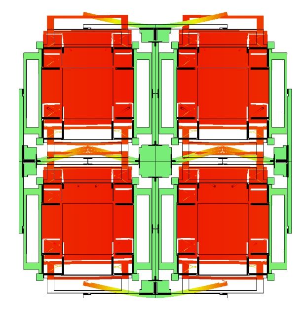
Micromachines 2021, 12, 266                                                                                                     4 of 25

                              Table 1. Progression of QMG performance characteristics.
                                                                                                                √
                                 Iteration           freq. [Hz]          Q-factor          ∆f [Hz]   ARW [◦ /       hr]        Ref.
                                  QMG-I                 2177               1.17M             0.2           0.06                [19]
                                  QMG-II                3047                 980            0.15        0.02–0.05              [32]
                                  QMG-III               2085                1.1M             0.2           0.04                [33]

                              Table 2. Characteristics of the three sensors used for the noise performance analysis.

                                                                                                                 ∆ f [Hz]
                                   Device ID              Q-Factor *             Drive Frequency [Hz]
                                                                                                             (as-Fabricated)
                                     DUT1                    1050                          2040                            4
                                     DUT2                   25,750                         2100                           25
                                     DUT3                 2,036,000                        1673                           15
                              * The difference is due to different packaging conditions.

                                   In this work, we discuss the noise performance and the effect of vacuum sealing on
                              QMGs with three different Q-factors, ranging from a 1000 (DUT1) to a 2,000,000 (DUT3),
                              Table 2. DUT3 with the highest Q-factor was used to demonstrate capabilities of the QMG
                              design and MEMS technology. The reported devices were instrumented to operate in the
                              rate mode.
                                   The material of this paper is organized as follows. In Section 2, we present a discussion
                              on the structural design of QMG, using as an example DUT3. In this section, we also
                              introduce the electrostatic scheme for actuation and detection of the orthogonal modal
                              frequencies and present the initial frequency response characterization. We will also
                              investigate the identification of the energy dissipation mechanisms in a QMG sensor. In
                              Section 3, we report a procedure of electrostatic tuning of the frequency split, as well as
                              analyze and discuss strategies for implementation of control algorithms and selection
                              of control parameters for sensors with different Q-factors. The limitations of a high-Q
                              mode-matched MEMS CVG in terms of the scale-factor nonlinearity and measurement
                              bandwidth in the open-loop rate and force-to-rebalance rate modes are experimentally
                              analyzed in Section 4. In Section 5, a discussion on noise performance analysis of DUTs in
                              the open-loop rate mode is presented and compared to the FRB rate mode of operation. The
                              same section discusses two methods for deriving ARW and bias instability from the Allan
                              Deviation (ADEV) and the Power Spectral Density (PSD) analysis. Both methods identified
                              and modeled random errors of the gyroscope output, where ADEV was extracted from the
                              time-domain data and PSD was extracted from the frequency-domain data. Furthermore,
                              finally, stability of the drive resonance frequency is characterized and correlated to noise
                              performance of the device. Section 7 concludes this paper with summary and outlook.

                              2. Quad Mass Gyroscope (QMG)
                                    A QMG comprises four coupled identical oscillators, providing an X-Y symmetry of
                              the resonant structure [34]. The coupled oscillators have four degenerate resonance modes:
                              (1) anti-phase, (2) in-phase, (3) double anti-phase, and (4) double in-phase, Figure 3. The in-
                              phase and double anti-phase modes are not independent and are coupled by the Coriolis
                              force, thus they are not utilized for gyro operation in the QMG design. The anti-phase and
                              double in-phase modes are independent and sensitive to the Coriolis coupling and can be
                              used for gyro operation. However, the double in-phase mode is sensitive to external linear
                              accelerations and should be avoided as the operational mode. The anti-phase motion of
                              masses during the operation assures minimization of the total reaction forces and moments
                              at the anchors, resulting in reduction of energy losses through the substrate, and therefore
                              the preferential mode for gyro operation [35].
Micromachines 2021, 12, 266                                                                                                5 of 25

                                 anti-phase           in-phase        double anti-phase double in-phase
                                   1680 Hz           2690 Hz              3475 Hz          4080 Hz
                                  (desired)         (undesired)         (undesired)       (undesired)
                              Figure 3. Eigen-frequency simulations of a Quad Mass Gyroscope (QMG), showing the four degener-
                              ate modes of vibration and the frequency of each resonance mode. The vibrational modes are ordered
                              to place the desired anti-phase mode at the lowest frequency [31].

                                   QMGs have one operational mode and three parasitic vibrational modes, which are
                              sensitive to external linear and angular accelerations. In order to suppress sensitivity
                              to environmental shock and vibrations and improve mechanical stability of the sensor’s
                              structure, the order and frequency of vibrational modes were designed using suspension
                              elements for mode-ordering, [29]. Four outer lever synchronization mechanisms and four
                              pairs of inner secondary beam-coupling elements were incorporated in the suspension
                              design to couple the proof-masses (see Figure 4). Advantages of these features of the
                              design included widening of the frequency separation between desired anti-phase modes
                              and parasitic in-phase modes, while shifting the in-phase modes to higher frequencies for
                              common mode rejection of linear accelerations, decreasing the mode conversion losses and
                              decreasing the drift induced by external vibrations.

                              Figure 4. Four external lever mechanisms and four pairs of internal secondary beam resonators,
                              responsible for ordering the eight vibrational modes of a QMG and for placing the desired anti-phase
                              mode at the lowest frequency [36].

                                   While the anti-phase operation was intended to reduce the energy dissipation and
                              improve the Q-factor along each orthogonal axis, the symmetric structure of the device
                              provided a damping and stiffness symmetry, which was shown to improve the overall
                              performance of the gyro operating in both the rate and the rate-integrating modes [18].
                                   QMGs that were used in this study were fabricated using a Silicon-on-Insulator (SOI)
                              process with a 100 µm device layer, 5 µm buried oxide layer, and a 500 µm handle wafer.
                              In this design, the mass of each tine was ∼1.4 × 10⁻⁶ kg, the width of suspension beams
                              was 10 µm, and the minimum trench width was 7 µm. The total footprint of the device was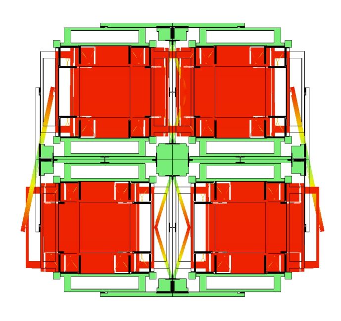
Micromachines 2021, 12, 266                                                                                                6 of 25

                              8.6 mm × 8.6 mm. The devices were diced and individual sensors were attached to ceramic
                              Leadless Chip Carrier (LCC) packages using eutectic bonding [37].
                                   The sensors consisted of 16 pairs of differential parallel-plate electrode arrays with
                              7 µm capacitive gaps for excitation and detection of the drive and sense modes. Every
                              four pairs of differential electrodes cover one proof-mass. In four-mass symmetric con-
                              figuration, differential electrodes for drive are located on the outer side of the structure,
                              and differential electrodes for sense are located on the inner side of the structure. Alto-
                              gether, the parallel-plates formed 3.7 pF active capacitance between the proof-mass and
                              the differential electrodes for each X- and Y-modes. The differential drive signals were
                              applied to all four masses symmetrically. For example, along the X-axis for the bottom
                              two masses, the in-phase drive signal (+) was applied to the outer most electrodes and
                              the out-of-phase drive signal (−) was applied to the inner electrodes; this configuration
                              is reversed for the top two masses. The differential sense signals from all masses were
                              lumped to one pickoff signal of the detection circuit. Figure 5 shows the arrangement of
                              electrodes for excitation and detection of the anti-phase mode of motion. The differential
                              pairs of electrodes were labeled (“+” and “−”), for both the drive (Dx and Dy) and the
                              sense (Sx and Sy) electrodes. These electrodes were wirebonded, such that they summed
                              under the same subset (e.g., the Dx+ signal arrives in the LCC package to 4 different pads
                              and distributes to 4 electrodes).

                                               Dy+                            Dy−
                                               Dy−                            Dy+
                                                     Y-mode

                                                                             X-mode
                                                                    Y-mode
                                                              Sx+
                                                              Sx−
                                                              Sx−
                                                              Sx+
                               Dx−
                               Dx+

                                                                                        Dx+
                                                                                        Dx−

                                       X-mode
                                               Sy−                           Sy+
                                               Sy+                           Sy−
                                               Sy+                           Sy−
                                               Sy−                           Sy+
                                                                               Y-mode

                                              X-mode
                                     Y-mode
                               Dx+
                               Dx−

                                                                                        Dx−
                                                                                        Dx+
                                                              Sx−
                                                              Sx+
                                                              Sx+
                                                              Sx−

                                                                         X-mode
                                               Dy−                            Dy+
                                               Dy+                            Dy−

                              Figure 5. Layout of the QMG structure with symmetric features: identical proof-masses and identical
                              drive and sense electrode structures overlaid with external forcers and internal pickoff electrodes,
                              which are used to drive and sense each mode separately.

                              2.1. Frequency Response Characterization
                                   The initial frequency response characterizations were carried out using a custom
                              analog signal conditioning printed circuit board, utilizing a charge amplifier (AD8034 Op
                              Amps) with a feedback resistor (1 -MΩ Vishay resistor), for capacitive detection. An HF2LI
                              lock-in amplifier from Zurich Instruments was used for the experiments. An Electromechan-
                              ical Amplitude Modulation (EAM) scheme was utilized to remove parasitic feedthrough
                              from the forcer to pickoff electrodes [38]. A 100 kHz carrier signal was applied to the
                              proof-masses and balanced by DC biases on all drive electrodes (equal DC voltages were
                              applied to all differential drive pair electrodes, Dx and Dy). An AC drive signal generated
                              by the network analyzer was applied to the drive electrodes, a differential pair Dx for the
                              X-axis or a differential pair Dy for the Y-axis. The amplitude of the pickoff signal was
                              estimated after demodulation at the carrier frequency and the drive frequency. The phase
                              of the delayed carrier was initially set to 0, while the amplitude of the pickoff signal was
                              monitored. A slightly delayed carrier was used for demodulation, allowing for an optimal
Micromachines 2021, 12, 266                                                                                                      7 of 25

                              phase setting of the EAM. The frequency response along the X-axis and Y-axis are plotted in
                              Figure 6, demonstrating an anti-phase resonant frequency at 1673 Hz and an as-fabricated
                              frequency mismatch of 15 Hz. The frequency mismatch was electrostatically tuned down
                              to 60 mHz (36 ppm) using 16.58 Volts DC bias applied to the sense electrodes along the
                              X-axis, with the resolution of 3.5 digits of the power supply, Figure 7.

                                                           0
                                                                                        0
                                                                                      −20
                                                        −20
                                      Amplitude (dBV)

                                                                                      −40
                                                                                      −60
                                                        −40
                                                                                      −80
                                                                                       1672   1672.5    1673   1673.5   1674
                                                        −60
                                                                      Y-mode                  X-mode
                                                        −80

                                                        −100
                                      Phase (deg)

                                                         100
                                                           0
                                                        −100
                                                          1500        1600          1700               1800               1900
                                                                               frequency (Hz)

                              Figure 6. Experimental results of the anti-phase drive (X-mode) and the sense (Y-mode) frequency
                              responses. Illustrating the increase in amplitude spectral density near the resonance frequency of
                              the modes.

                                                                 Experimental results on frequency tuning
                                                1690
                                                                                                       X-mode
                                                1685                                                   Y-mode
                                                                                                       -exp data points
                              Frequency (Hz)

                                                1680

                                                1675

                                                1670

                                                1665
                                                           0           5           10           15                        20
                                                                             tuning voltage (V)
                              Figure 7. Experimentally obtained frequency response of the QMG showing the frequency separa-
                              tion changes between the orthogonal axes by applying DC bias to the X-mode pickoff electrodes.
                              Illustrating the X-mode resonance frequency decreases with increase tuning voltage while Y-mode
                              resonance frequency keeps unchanged.

                              2.2. Q-Factor Measurement
                                   Using the same setup as described in Section 2.1, the Q-factor was estimated by
                              measuring the ringdown time. The ringdown time, τ, is defined as the time that it takes for
                              the settled drive amplitude to drop down to 1/e of the initial drive amplitude under free
                              vibration [39], and is measured in seconds. This parameter is used to extract the Q-factor,
                              Q = π f τ, where f is the resonant frequency measured in Hertz.
                                   In MEMS resonators and CVGs, the Q-factor is a figure of merit and a measure of
                              the overall damping from all possible loss mechanisms in a system. The primary energy
Micromachines 2021, 12, 266                                                                                            8 of 25

                              dissipation mechanisms in MEMS resonant structures are viscous damping, Thermoelastic
                              Damping (TED), anchor loss, surface-related losses, and electrical damping [40]. The overall
                              Q-factor is the reciprocal sum of Q-factors from different loss mechanisms and is limited
                              by the dominant loss mechanism in the system:

                                                        Q− 1      −1          −1     −1         −1
                                                         Total = QViscous + Q TED + Q Anchor + QOthers .                  (2)

                                   In order to suppress the effect of viscous damping, the DUTs were sealed using an
                              Ultra-High Vacuum (UHV) sealing process [37]. For vacuum sealing of sensors, LCC
                              packages were pre-baked at 400 °C in a vacuum furnace for 7 h in high vacuum (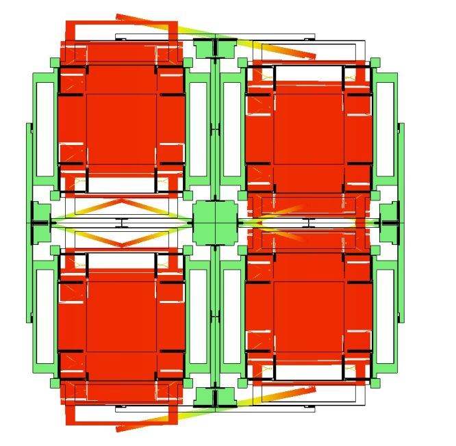
Micromachines 2021, 12, 266                                                                                                        9 of 25

                                                                                Ringdown experiment
                                                             1
                                                            0.8

                               Normalized amplitude (log)
                                                            0.6

                                                                                                        378   382    386   390
                                                            0.4

                                                            0.2
                                                                      Qx = 2,036,000, τx = 383.7 (s), fx= 1,689 Hz
                                                                      Qy = 2,029,000, τy = 386.1 (s), fy= 1,673 Hz
                                                            0.1
                                                                  0   100     200     300         400          500           600
                                                                                     time (sec)

                              Figure 9. Ringdown time measurements revealed the Q-factor as high as 2 million, on both X-axis
                              and Y-axis, after UHV sealing.

                              3. Performance Analysis
                                   In this section, the statistical analysis of the Zero Rate Output (ZRO) of three QMG
                              sensors with different Q-factors and different levels of symmetry, but similar operational
                              frequencies, are discussed. The purpose of this analysis is to provide insight into factors
                              contributing to lower noise performance by identifying device-specific error parameters,
                              and subsequently analyze the effect on control algorithms, and relate to complexity of
                              control algorithm implementations. The variation in the Q-factors of DUTs is attributed
                              to the different vacuum sealing conditions. DUT 1 and DUT 2 were packaged without
                              getter with a pre-bake duration of 4 h and 12 h, respectively. DUT 3 was packaged with
                              a pre-bake duration of 24 h and getter activation. Using the Q-factor measurements at
                              different pressures in a vacuum chamber prior to the vacuum sealing, the residual cavity
                              pressure for DUT 1, 2, and 3 were estimated to be ∼1 Torr, ∼40 mTorr, and
Micromachines 2021, 12, 266 10 of 25
1690
(X-mode)
1689 −23.7 ppm/°C
1688
1687
Frequency (Hz)
1674 (Y-mode)
−24.5 ppm/°C
1673
1672
1671
20 30 40 50 60
temperature (°C)
Figure 10. Experimental results of the TCF along X-axis and Y-axis of the sensor with as-fabricated ∆ f
of 15 Hz. The measurement was performed in a thermally-controlled environment, with temperature
ranging from 25 to 55 °C, and temperature fluctuations within 0.04 °C at each measurement point.
In the nearly-matched frequencies, the ∆ f was extracted by FFT spectrum analyzer
of oscillations along the drive axis. Figure 11 shows an extracted ∆ f using the procedure,
confirming the ability to reach an optimal tuning voltage value at 16.15 V, achieving
∆ f < 1 Hz. The inset plot illustrates examples of PSD with three DC voltage levels (A, B,
C) at 15.80, 16.15 and 17.35 V, with an estimated ∆ f of 250, 60 and 1900 mHz, respectively.
The described method enables a real-time observation of the ∆ f for high Q-factor devices,
while actively adjusting the applied DC tuning voltage.
Frequency tuning
101
│Frequency split│ (Hz)
C
61(mHz) B A
100 C
A
10−1 61(mHz)
B
Δfrequency (Hz)
10−2 10−1 100 101
−2
10
0 5 10 15 20
tuning voltage (V)
Figure 11. Estimation of |∆ f | by monitoring the peak in the power spectrum of the nearly-matched
region for a high Q-factor device. Inset figure shows the PSD of the drive signal at the corresponding
reference points. Results are experimental.
The variation in the width of spring elements across a die due to fabrication imperfec-
tions results in a misalignment between the orientation of the principal axis of elasticity and
the orientation of electrostatic forces along the drive and sense axes defined by the layout.
Due to asymmetry and misalignment of axes, non-zero off-diagonal components appear
in the stiffness matrix. The achievable tuning accuracy of frequency mismatch depends
on the off-diagonal stiffness and the nominal frequency of operation. Compensation of
off-diagonal stiffness using electrostatic spring softening requires tuning electrodes alongMicromachines 2021, 12, 266 11 of 25
45 degree orientation with respect to drive and sense. Figure 12 illustrated the frequency
mismatch accuracy versus ratio of off-diagonal to diagonal stiffness in part per million for
different resonant frequencies. The level of imperfection in DUTs were not identical since
different processes were used for their fabrication.
3
10
z
DUT 1 1 MH
DUT 2
minimum frequency split (Hz)
2
10 DUT 3 Hz
100 k
1
10 z
10 kH
0
10 z
1 kH
−1
10
−2
10
1 2 3
10 10 10
off-diagonal/diagonal stiffness (ppm)
Figure 12. Minimum of frequency split (∆ f ) between drive and sense modes as a function of
off-diagonal stiffness. Straight lines represent different drive oscillation resonant frequencies.
3.2. CVG Control Algorithm
The CVG control algorithm was implemented based on the IEEE Std 1431 [44]. The dig-
ital control of the characterization was carried out using the HF2LI lock-in amplifier. Four
primary control loops were implemented for the rate mode characterization, including
Phase-Locked Loop (PLL), Amplitude Gain Control (AGC), Quadrature Control Loop
(QCL), and Rate Control Loop (RCL), Figure 13. Each loop comprises: (1) a demodu-
lator for demodulating a received signal from the device, either along X-axis or Y-axis,
into in-phase (cos) or in-quadrature (sin) signals, (2) a low pass filter (LPF) for passing
only low-frequency component, (3) a PID controller with a set point for controlling the DC
component of the demodulation, and (4) a modulator for modulating the controlled signal
to a higher frequency defined by the local reference oscillator signal. The PLL loop has
two extra components, which are Phase Detector (PD) and Voltage-Controlled Oscillator
(VCO). Using these control loops, a gyro can be configured to operate in the open-loop
rate mode under the following conditions: (a) PLL only, (b) PLL and AGC, (c) PLL, AGC,
and QCL, or (d) closed-loop rate mode where all four loops (PLL, AGC, QCL, and RCL)
are established, also known as closed-loop FRB rate mode.
The PLL generates a reference frequency by tracking the resonant frequency of the
drive mode, which is done by a VCO with negative feedback to a phase detector. The phase
detector compares the phase of the received signal with respect to the local oscillator and
generates an error signal; the PLL is called “locked” when the error signal is zero. The AGC
loop maximizes the in-phase component of the drive signal to a pre-defined set point value,
and the QCL loop nulls the in-quadrature component of the sense signal. The RCL loop
is used to estimate the input rate from the in-phase component of the sense signal in the
open-loop configuration, or from the voltage applied to null the rate signal in the FRB
rate mode.Micromachines 2021, 12, 266 12 of 25
X-axis cos
carrier
PD VCO sin
+
LPF
Px sin PLL
C/V Buff.
+
LPF
Fx
+
PID
+
+
Fx LPF
Buff. carrier cos Amp sin AGC
Fy
Buff. estimate
PID quadrature
+
+
Fy LPF
sin cos QCL
C/V Buff.
+
Py LPF estimate Fy
PID rate
+
+
carrier LPF
Y-axis cos sin RCL
Figure 13. Control structure for operating devices in the rate mode. AGC and PLL were activated
along the drive axis of the device (X-mode). QCL and RCL were activated along the sense axis of the
device (Y-mode).
3.3. Control Accuracy
In this section, we highlight challenges in stabilization of the control loops for devices
with different levels of symmetry and the quality factor, and derive the corresponding
hardware requirements. A PID controller is needed to track and stabilize the amplitude in
the drive direction, phase of the drive oscillation frequency, amplitude of the quadrature
and rate parameters in the sense direction from demodulated components of the drive and
sense signals (also known as slowly-varying parameters). The general PID equation can be
represented by: Z
u = KP e + K I e + K D ė , (3)
where u is the control signal, e is the control error, and the controller parameters are K P
(proportional), K I (integral) and K D (derivative) gains of the linear control architecture.
In this work, only the PI controller was used for feedback to stabilize parameters (ampli-
tude, phase, quadrature, and rate feedback). Each controller has a set point, bandwidth,
and sampling rate. Experimental results revealed that the PI parameters for a low Q-factor
device (high loop bandwidth) would fail to control the high Q-factor devices (low loop
bandwidth), and vice versa. Applying PI parameters, which were selected for a high
Q-factor device, to a low Q-factor device would result in a slower response, which is unfa-
vorable for fast frequency tracking. Consequently, the loop bandwidth has to be set based
on the device parameters. These parameters for the three selected devices (DUT1-DUT3)
were set as follows: the −3 dB cutoff frequency of the loop filter in the PLL was selected
to be around 100 Hz, centered at the resonant frequency of the drive axis. A phase shift
occurred between the driving mass forcer signal (denoted by Fx in the diagram shown in
Figure 13) and the phase detector in the PLL loop (marked as PID block in the diagram
shown in Figure 13). The signal path includes a preamplifier buffer circuit, the device,
a charge amplifier, a front-end buffer circuit, a carrier demodulation circuit, and a LPF.
The phase setpoint of the PLL aligns this phase shift of the feedback signal with the forcer
signal. The transfer function of a resonator PLL system dynamics is [45]:
1
Φ(s) = , (4)
( t c s + 1)
where Φ is the resonator’s phase and tc = 2Q/(2π f ) is the exponential time constant.
The output propagates to a low-pass filter, where the controller adjusts the phase Φ. The PI
parameters of the PLL unit are responsible for the fast lock of the resonance frequency to
the reference local oscillator. The high Q-factor resonators require a narrower bandwidth
(BW = 1/tc ), on the order of Q inverse, due to the transfer function characteristics of theMicromachines 2021, 12, 266 13 of 25
system, whereas in low Q-factor resonators the bandwidth is much higher, again on the
order of Q inverse.
For the DUTs in this study, the setpoints for the rate and quadrature loops were
selected to be 0 Vrms and for the drive amplitude were selected to be 0.42 Vrms, to utilize
the full-scale resolution from the amplifier output to the Analog-to-Digital Converter (ADC)
with an input range of ±1.2 Volts.
To achieve the target bandwidth and stable loop conditions, different sets of PI param-
eters (units for K P are [V/Vrms] or [Hz/deg], and for K I are [V/Vrms/s] or [Hz/deg/s])
were selected and verified experimentally for devices with different Q-factors. For a Cori-
olis vibratory gyroscope in a self-oscillation mode (or using an external signal generator
from PLL), the Routh-Hurwitz criterion to satisfy the stability is [46]:
m x 2π f x
KP > ,
Gp G f Qx (5)
ωc K P > K I ,
where G p and G f are the gain buffer after pickoff and generated forcer signals, and ωc is
the cutoff frequency parameter of the LPF of the loop. The G p parameter was fixed across
the three DUTs, but G f was adjusted accordingly and was selected to be lower when the
Q-factor was higher. Thus, K P is inversely proportional to the Q-factor and the G f . Given
the above parameters and initial settings for each loop, K P and K I were implemented
and results are shown in Figure 14. The figure illustrates the sensitivity constraints on
the magnitude of the four primary CVG control loops vs. frequency. In the closed-loop
configuration, the integrator’s coefficient K I stabilizes the proportional controller and
zeros the steady-state error. As expected, the crossover integrator frequency (closed-loop
bandwidth) component decreased as the device’s resonance Q-factor increased. Overall,
the PI parameters of the control loop need to be adjusted based on the Q-factor of the device,
affecting the speed of the control loops. The sampling rate of the input signals to the four
primary CVG control loops (PLL, AGC, QCL, and RCL) were set to be at 130 kHz (between5
and 10× of the device’s resonance frequency). In our experiments, the sampling rate of
the PI digital controller run one order of magnitude faster than the crossover frequency,
ensuring that any changes in the signal can be controlled.
Amplitude Loop Phase-Locked Loop
60
Q = 1k
40
Magnitude (dB)
Q = 25k
20 Q = 2M
0
−20
−40
−60
Rate Loop Quadrature Loop
60
40
Magnitude (dB)
20
0
−20
−40
−60
10 −4 10 −2 10 0 10 2 10 4 10 −4 10 −2 10 0 10 2 10 4
frequency (Hz) frequency (Hz)
Figure 14. Illustrated configurations of PI parameters on the amplitude (AGC), phase (PLL), quadra-
ture (QCL) and rate (RCL) loops for QMG devices with Q-factors ranging from 1000 to 2,000,000. PI
parameters were scaled proportionally to the Q-factor of the device. Results are experimental.Micromachines 2021, 12, 266 14 of 25
3.4. Open-Loop Operation in the Rate Mode
In the open-loop CVG rate mode of operation, the drive mode was excited to a fixed
amplitude A0 , with the use of AGC, and at the frequency f x , and with the use of PLL. Due
to the Coriolis coupling, the input rate causes the excitation of the sense mode channel,
and the sense mode amplitude is proportional to the input rate.
The scale-factor was extracted by applying a reference rotation using a rate table,
with incremental step inputs of 0.25 °/s in the clockwise and counter-clockwise directions.
The open-loop scale-factor of 2.2 mV/(°/s) was obtained for the high Q-factor device.
Figure 15 illustrates the device response over time for a small input rotation range, where
the inset plot shows linearity of the input-output of the same dataset.
Scale-factor measurement
2
0.75o/s
1.5 0.60o/s
0.45o/s
1
0.30o/s
Gyroscope output (mV)
0.5 0.15o/s
0o/s
0
o
2 −0.15 /s
Slope:
−0.5 1 −0.30o/s
2.2 mV/(°/s)
0 −0.45o/s
−1
−1
−0.60o/s
−1.5 −2
−1 −0.5 0 0.5 1
input rotation (°/s)
−0.75o/s
−2
0 100 200 300 400 500 600 700
time(sec)
Figure 15. Characterization of angular rate response to clockwise and counter-clockwise rotation
with different step-input amplitudes of 0, ±0.15, ±0.30, ±0.45, ±0.60 and ±0.75 °/s, revealing an
open-loop scale-factor of 2.2 mV/(°/s).
3.5. Force-to-Rebalance Operation in the Rate Mode
Similar to the open-loop, in the closed-loop CVG the drive mode was excited to a
fixed amplitude A0 , with the use of AGC, and at the frequency f x , with the use of PLL.
An additional force was applied along the sense mode to null the response. This force
is required to null the sense mode amplitude and is proportional to the input rate, thus
the architecture is called Force-to-Rebalance (FRB) or closed-loop instrumentation of CVG
operating in the rate mode.
The scale-factor extraction is similar to the described open-loop architecture, and,
similarly, the ZRO data could be used for noise analysis. Due to inconsistencies in the
sampling time interval during data recording of the Digital-to-Analog Converter (DAC)
components of the hardware setup, the noise performance of the gyroscope’s output rate
in the FRB mode was estimated from the input to the RCL loop (open-loop rate estimate)
ADC component multiplied by inverse of the loop gain, rather than the output of DAC
component (Fy signal, shown in Figure 13). However for the scale-factor, the output was
estimated from DAC component from maximum and minimum fluctuation response, even
though with sampling time inconsistency. The FRB rate voltage output was then converted
to an equivalent rotation rate in °/s.
4. Scale-Factor Nonlinearity and Bandwidth
The advantage of high-Q MEMS CVGs operating in the mode-matched condition is a
high sensitivity to the input rotation and its ability to measure low angular rates. However,Micromachines 2021, 12, 266 15 of 25
the linearity of the scale-factor [47] and the measurement bandwidth [48] are limited when
the sensor is operating in the open-loop rate mode. The scale-factor linearity and the
bandwidth limit of the sensors operating in the open-loop and closed-loop modes were
characterized experimentally.
For linearity analysis, an input rotation in the range of angular rates from 0 °/s to
1080 ◦ /s with an increment of 60 °/s was applied using an Ideal Aerosmith 1571 rate table.
The linearity of the input-normalized output under different loop configurations were
compared experimentally only for the DUT1 operating in the mode-matched condition,
Figure 16. DUT1 with low Q-factor was selected for flexibility of adjusting parameters
and repeating the experiment at several input angular rotations. The results demonstrated
that the linear range of operation is limited in the open-loop operational mode, that is
when only the drive axis control loop PLL was established. The linear range increases
when both PLL and AGC were activated. An extended scale-factor linearity was observed
when devices operated in the closed-loop sense configuration (FRB). Based on these results,
the FRB fully compensates for nonlinearity in the output response for the input rotation
range from 0 to 3 Hz. It is expected to see a similar trend for DUT2 and DUT3 by activating
individual control loops, however with a smaller linear region due to quality factor of
these samples.
Scale-factor nonlinearity
3
FRB
PLL & AGC & Quad
2.5
Gyroscope output (Hz)
PLL & AGC
PLL
2
1.5
1
0.5
0
0 0.5 1 1.5 2 2.5 3
input rotation (Hz)
Figure 16. Experimental measurements of the scale-factor nonlinearity in DUT1, operating in the
mode-matched condition with different configurations of control loops.
Next, we repeated measurements in the open-loop configuration, when control loops
(PLL and AGC) were activated across all three DUTs. Figure 17 demonstrates the scale-
factor nonlinearity in the open-loop rate mode for devices with different Q-factors, op-
erating in the mode-matched (or nearly-matched) condition. As expected, the linear
input-output range of operation becomes narrower as the Q-factor increases, confirming
the sensitivity of resonator’s bandwidth in the open-loop operational mode relative to its
drive frequency over Q-factor, f x /Q.
In a mode-matched device, the bandwidth is determined by the Q-factor of the device,
whereas for a mode mismatched device the BW is dominated by the ∆ f [49]. Generally,
a higher bandwidth can be achieved by increasing the damping coefficient (lowering
the Q-factor) or operating in the mode-mismatched condition (increasing the frequency
mismatch ∆ f ), [50]. We support this observation by a diagram shown in Figure 18. In the
diagram, the parameters for the drive amplitude ( A) and the mass (m) are grouped as
G1 = –2 mAΩ, and the circuit and buffer gains are grouped as G2. The notations Fy (i ) andMicromachines 2021, 12, 266 16 of 25
Fy (q) represent the in-phase and in-quadrature forces applied along the sense axis of the
device. The input drive voltage F (t) along the sense axis in the open-loop case is
F (t) = −2mAΩsin(wx t) + Fq cos(wx t), (6)
and in the closed-loop (FRB) case is
F (t) = −2mAΩsin(wx t) + Fq cos(wx t) + Fy (q) + Fy (i ). (7)
Scale-factor (AGC + PLL)
3
2.5
10−1
Gyroscope output (Hz)
2
10−1
1.5
Q = 1k
Q = 25k
1 Q = 2M
Linear fit
0.5
0
0 0.5 1 1.5 2 2.5 3
input rotation (Hz)
Figure 17. Experimental results of the scale-factor nonlinearity in sensors with different Q-factors and
mode-matched condition, operating in the open-loop rate mode (PLL and AGC loops are enabled).
sin(wxt) Fq=cos(wxt) Fy(q)
PID
+
+
LPF
Sense mode sin cos
Ω(t) G1 + G2 Open-loop
+
(wy , Q)
Fy(i)
PID
+
+
Fy(i) + Fy(q)
cos
LPF
sin
Figure 18. Simplified block diagram of the open-loop and closed-loop rate QMG MEMS gyroscope.
The Laplace transform of each of the shown components are as follows:
1/M
Sense(s) = ,
s2
+ (wy /Q)s + w2y
wc
LPF (s) = ,
s + wc
K (8)
PI (s) = K P (1 + I s),
KP
OL(s) = Sense(s) LPF (s) F (s),
FRB(s) = (OL(s) PI (s))/(1 + OL(s) PI (s)).
To filter out the excitation amplitude of the sense mode resonance, the selection of
the LPF cutoff frequency wc is typically 3 times lower than the ∆ f . The selection of the PI
controller gains K P and K I are also device dependent and were discussed in Section 3.3.
The frequency analysis of the open-loop OL(s) and the closed-loop FRB(s) of the gyroscope
model with respect to the input rotation Ω(s) was performed in the Matlab environment,Micromachines 2021, 12, 266 17 of 25
and shown in Figure 19. The analysis was repeated on all three DUTs with different Q-
factors. For DUT1 and DUT2 with low and medium Q-factors, the open-loop BW analysis
shows a strong dependency to the frequency split, but for the DUT3 with a high Q-factor
of 2 M and ∆ f of 60 mHz, the –3 dB was dominated by the Q-factor of the device and
estimated to be 0.5 mHz, which is two orders of magnitude lower than the frequency
split. The BW limit observed in the open-loop operation can be compensated if the device
was operated in the FRB mode. Simulation of parameters of the three DUTs shows that
a higher BW is possible when FRB is selected as a preferable mode of operation. This
conclusion was also verified experimentally and shown in the graph of Figure 19. However,
this should be understood that the FRB amplitude range is limited to the DAC forcer
amplitude resolution.
Open-loop (OL) Closed-loop (FRB)
0 0
−50 −50
DUT1 ∆f DUT1
−100 −100
10 −4 10 −2 10 0 10 2 10 −2 10 0 10 2
Gyroscope output (dB)
0 0
−50 −50
−100
DUT2 ∆f −100
DUT2
10 −4 10 −2 10 0 10 2 10 −2 10 0 10 2
0 0
−50 −50
DUT3 ∆f DUT3
−100 −100
10 −4 10 −2
10 0
10 2
10 −2 10 0 10 2
frequency of input rate (Hz)
Figure 19. Simulation of the gyroscope bandwidth overlaid with experimental measurement points,
operating in the open-loop (first column) and closed-loop (second column). Three devices with
different Q-factors were used and each row represents one device.
The BW of the QMG sensors were experimentally derived. Sinusoidal stimulus
commands with varied frequencies, from 0.01 Hz to 5 Hz, were applied to the rate table.
The experiment was repeated for the three sensors in the open-loop and the FRB rate mode
mechanizations, Figure 19. From the rate output measurement of each mode, the –3 dB
range resolution was extracted to be at 100, 227 and 790 mHz, which is in a close agreement
with the tuned ∆ f of the QMG devices under electrostatic tuning conditions of 450, 250
and 60 mHz, respectively. Operating the device in the FRB configuration resulted in a
higher bandwidth, independent from the frequency split of the device. This was confirmed
on DUT1 and DUT2. However, for the high Q-factor sensor (DUT3), and for the input
angular rate of rotation around 1 Hz, the FRB utilized the full amplitude range available
of the hardware along the sense axis of the device. Therefore, there was no enough force
authority to fully null the input rate above this limit, and the forcer signal along the sense
axis (Fy) was saturated, resulting in a faulty loop operation. This constraint resulted in
–3 dB loss at 1 Hz, Figure 19.Micromachines 2021, 12, 266 18 of 25
5. Noise Analysis
The breakdown of all noise processes in the ZRO output of a gyroscope can be
described by:
σT2 (τ ) = σARW
2
(τ ) + σB2 (τ ) + σQN
2 2
(τ ) + σRRW (τ ) + ... , (9)
where ARW, B, QN and RRW represent the Angle Random Walk, Bias Instability, Quanti-
zation Noise, and Rate Random Walk, respectively, and the corresponding Allan variance
σ2 at any given τ averaging time. To extract these noise parameters individually, two
statistical methods were used and compared, one in the time domain and another in the fre-
quency domain. We analyzed the amplitude fluctuations and signal power over frequency
of the rate output. Furthermore, the frequency stability was also analyzed to identify the
noise sources. These methods are discussed next.
5.1. Allan Deviation (ADEV)
To characterize the short-term stability of the gyroscope, a two-sample deviation
was measured over different time intervals. When the device was operated in the rate
mode, the higher the Q-factor of the sense mode and the lower the frequency split between
the drive- and the sense-modes, the lower ARW and a higher signal-to-noise ratio of the
gyro response. In a still condition (no input rotation was applied), data was recorded
for 16 h with the sampling rate of 10 Hz in the form of in-phase and in-quadrature data
samples. The recording length was enough to provide an estimated ARW with 0.2% error
from the ADEV plot, bias, and RRW. The data collection for the ZRO experiment was
conducted in a lab environment without any thermal compensation. Frequency mismatch
ofMicromachines 2021, 12, 266 19 of 25
Allan deviation, σy(τ)
10 1
(a)
(b)
Deg/hr
10 0
(c)
10 −1
(d)
Navigation grade
10 −2
10 −1 10 0 10 1 10 2 10 3 10 4
averaging time, τ (sec)
Figure 20. Noise characteristics of QMG with different Q-factor conditions with curve fit lines
estimating ARW (slope –1/2), bias instability (slope 0) and RRW (slope +1/2) for QMG in the open-
loop operation for (a) Q = 1k, (b) Q = 25k, (c) Q = 2M, and (d) in the closed-loop (FRB) operation
mode, Q = 2M.
Table 3. Summary of device parameters and noise characteristics.
Device ID DUT1 DUT2 DUT3 DUT3
Mode of Operation OL OL OL FRB
Quality factor (Q-factor) 1k 25k 2M 2M
∆f (tuned) [Hz] 450 m 250 m 60 m 60 m
SF [V/(◦ /s)] 85.7 µ 790 µ 2.2 m 2.6 m
offset [◦ /hr] 3.0542 1.0873 1.9497 -
√ ADEV 0.1770 0.0843 0.0107 0.0058
ARW [◦ / hr]
PSD 0.1177 0.0576 0.0080 0.0038
ADEV 2.0907 0.5096 0.0946 0.0655
Bias Instability [◦ /hr]
PSD - 0.3938 0.0459 0.0647
√
RRW [◦ /hr/ hr] ADEV 0.1256 0.0300 0.0043 0.0107
In the PSD analysis, the ARW component white noise is typically dominated and
can be estimated well with a fit line (slope 0), whereas in the ADEV analysis the bias is
dominated and estimated well with a line fitting (slope 0). In PSD, the estimation accuracy
was reduced in the plot for low-frequency bins. In contrast, in ADEV, the uncertainty
increased for long averaging time intervals.
Figure√21 shows this analysis and for a high Q-factor device it revealed the ARW
of 0.008 °/ hr and the bias of 0.0459 °/hr. However, using the time domain integration
on the same
√ dataset, the bias instability was estimated
√ to be 0.0946 °/hr, the ARW to be
0.0107 °/ hr, and the RRW to be 0.0043 °/hr/ hr.
Both described methods are offline and require post-processing of the stored data.
To demonstrate the effectiveness of both methods, the high Q-factor data was segmented
into durations of 0–10 min, 0–20 min, 0–30 min, etc., all the way to 0–16 h, and then theMicromachines 2021, 12, 266 20 of 25
ADEV and the PSD analysis were repeated. Both methods showed that the confidence of
the estimated stability parameters improved as more data points were fed to the analysis.
The high Q-factor data shows that the optimal size for bias estimation would reach 10%
of its final value in 10 h for the ADEV method (Table 3), and from the PSD method in 7 h.
Similarly, for the ARW estimation, 10% of its final value was reached in 3.5 h using the
ADEV method, and in 5 h using the PSD method.
Single-sided PSD
10 2
PSD [(deg/hr)2/(Hz)]
(a)
10 1
(b)
(c)
10 0
(d)
10 −3 10 −2 10 −1 10 0 10 1
frequency, (Hz)
Figure 21. Rate PSD of static QMG data with curve fit lines estimating ARW (slope 0) and bias
(slope –1). Lines (a–d) represent the same dataset and labelled in the time-domain analysis of
Figure 20. Data sample rate is 10 Hz.
5.3. Frequency Stability
The stability of the drive mode oscillation at the resonance is a critical parameter as it
directly relates to the scale factor of the device. Frequency and phase are related to each
other by 2π, meaning that any instantaneous frequency changes (δ f ) in the drive mode
are wrapped by 2π to maintain the phase changes (δΦ). For an oscillator, the instability
can be approximated by δ f / f ≈ −δΦ/2Q, where δ f is a fluctuation in the drive oscillator
frequency and δΦ represents changes in the phase [53]. Stability of the oscillator frequency
is proportional to the Q-factor. The variation in oscillations along the drive axis was
analyzed experimentally. The fluctuation in frequency or phase resulted in a phase error in
the drive mode of oscillation, therefore a high Q-factor is desirable to minimize this error.
In a simplified analysis, the CVG can be viewed as a two-dimensional oscillator, where
in the rate mode of operation, the output of the device is estimated from demodulation of
the sense axis with respect to the frequency of the drive mode, as defined by the PLL. In the
PLL, the phase is locked to the resonance center frequency in order to provide a reference
frequency signal. Therefore, variations within this frequency or phase can directly translate
to the phase error. Although it is outside the scope of this paper, it should be noted that
a mode-mismatched operation would be an alternative method for device operation and
would have its benefits, including less sensitivity to variations in demodulation phase.
The Allan deviation analysis on frequency stability (δ f / f ) provides an estimate of the
frequency noise processes. For inertial sensors, the frequency error is typically dominated
by the frequency white noise [54]. Since the relation between the frequency and the phase
is integral, as a result of integration, any small variation in frequency white noise (slope
–1/2) resulted in phase error (slope +1/2). Therefore induced drift in white noise frequency
contributes linearly to the RRW characteristics (slope +1/2) of the ZRO.Micromachines 2021, 12, 266 21 of 25
Figure 22 shows the frequency stability analysis of the QMG devices with different
Q-factors under the same room temperature environment, where the rate table operates in
an enclosed thermal
√ chamber. The frequency white noise was estimated to be 27.5, 1352.6
and 6072.5 ppb/ Hz, which is in a strong agreement with the experimentally obtained
RRW in Table 3. As expected, higher frequency stability was observed for devices with
high Q-factors. Thus, supporting the prediction that maximizing the Q-factor helps to
reduce environmentally induced noises in RRW (long term drift), including temperature
and other long-term variations in the drive oscillator.
Allan deviation, σ∆f/f (τ)
(a): Q=1k
10 4 (a) (b): Q=25k
(c): Q=2M
Frequency stability, ppb
10 3 (b)
10 2
(c)
10 1
10 −1 10 0 10 1 10 2 10 3
averaging time, τ (sec)
Figure 22. Characterization of the drive mode resonance frequency instabilities for three different
Q-factors. The frequency white noise improved as the Q-factor increased.
6. Discussion
The bias instability and ARW were optimized experimentally for the three DUTs
and the highest values were reported. The drive amplitude and electrostatic frequency
mismatch compensation were adjusted in an iterative process for each individual DUT to
achieve the best possible noise performance. Maximizing the Q-factor (>2 M) and reducing
the drive-sense frequency separation (Micromachines 2021, 12, 266 22 of 25
open-loop mode. The robustness against temperature variations requires operation in the
closed-loop control with an implementation of self-calibration. We identified the need for
continuous monitoring of frequency mismatch. As in the open-loop, the frequency of the
drive mode can be monitored through the PLL, but the sense mode frequency cannot be
conveniently accessed. One can use mode reversal (intervals of switching operation) in
FRB mode to extract and monitor frequency mismatches.
7. Conclusions
We presented the performance analysis of CVG devices, designed to operate in the rate
mode in the nearly mode matched configuration. The paper discussed the corresponding
control challenges involved. A highly symmetric device demonstrating the Q-factor of
above 2 million was compared to 1000 and 25,000 Q-factor devices of the same design.
The frequency split of all devices were electrostatically compensated to the lowest possible
level given the configuration of the electrodes in layout of the√DUTs. We demonstrated a
possibility of achieving 0.09 °/hr bias instability and a 0.01 °/ hr ARW in the rate mode
of operation in lab conditions (temperature fluctuations from 23.4 °C to 25.6 °C), with no
thermal compensations on the device level.
We described the structure of the CVG control algorithm and highlighted the hardware
requirements for implementation. The criteria to achieve stable control loop conditions
were examined on CVGs with different Q-factors. The dependence of the scale-factor non-
linearity on control loops was investigated in different combinations (PLL only, PLL+AGC,
PLL+AGC+QCL, and FRB), which resulted in a linear full-scale dynamic range in the
FRB mode. The tradeoff between bandwidth and sensitivity was investigated and shown
experimentally on a CVG with different Q-factors operating in the open-loop rate mode.
We verified and demonstrated that the frequency mismatch defines the operational band-
width of the CVG in the open-loop mode, where the highest sensitivity is demonstrated
for a lower ∆ f of mode mismatches. When the device was operated in the FRB mode, we
observed deviations from linearity in the bandwidth analysis for devices with different
Q-factors. We demonstrated that a higher Q-factor resulted in higher frequency stability,
thus in lower rate random walk. These outcomes were predicted by our analytic analysis
and supported in this paper experimentally.
We showed that a higher Q-factor and a lower frequency split can lead to the noise
performance improvement by >100 fold in ARW, bias, and RRW. We derived the noise char-
acteristic parameters, using both time domain and frequency domain analyses. Performing
analyses on the same dataset showed that the ADEV method leads to representation of data
with significantly lower noise characteristics compared to the PSD method, and should be
considered as a lower bound on the noise performance. Regardless of the Q-factor, uncer-
tainty in the noise parameters were lower on the flat portion (slopes 0, Figures 20 and 21),
that corresponded to bias instability in ADEV and ARW in PSD.
Author Contributions: Conceptualization, S.A., M.H.A. and A.M.S.; methodology, S.A., M.H.A. and
A.M.S.; software, S.A.; validation, S.A. and M.H.A.; formal analysis, S.A. and M.H.A.; investigation,
S.A. and M.H.A.; resources, A.M.S.; data curation, S.A. and M.H.A.; writing—original draft prepara-
tion, S.A. and M.H.A.; writing—review and editing, S.A., M.H.A. and A.M.S.; visualization, S.A. and
M.H.A.; supervision, A.M.S.; project administration, A.M.S.; funding acquisition, A.M.S. All authors
have read and agreed to the published version of the manuscript.
Funding: This material is based on work supported by the Defense Advanced Research Projects
Agency and U.S. Navy under Contract No. N66001-12-C-4035.
Data Availability Statement: The data presented in this study are available on request from the
corresponding author.
Acknowledgments: The authors would like to acknowledge the contribution of Kasra Kakavand
for assistance with post-fabrication processing. The QMG was conceptualized by Andrei M. Shkel,
Adam R. Schofield, and Alexander A. Trusov, and the mode-ordering mechanism was designed and
implemented by Brenton R. Simon which resulted in several patents on the topic. Methodology forYou can also read