PREDICTING ELASTIC PROPERTIES OF MATERIALS FROM ELECTRONIC CHARGE DENSITY USING 3D DEEP CONVOLUTIONAL NEURAL NETWORKS
←
→
Page content transcription
If your browser does not render page correctly, please read the page content below
P REDICTING E LASTIC P ROPERTIES OF M ATERIALS FROM
                                                         E LECTRONIC C HARGE D ENSITY U SING 3D D EEP
                                                              C ONVOLUTIONAL N EURAL N ETWORKS
arXiv:2003.13425v2 [cond-mat.mtrl-sci] 11 Apr 2020

                                                     Yong Zhao 1 ,Kunpeng Yuan2,3 , Yinqiao Liu 2,4 ,Steph-Yves Louis1 , Ming Hu 2,∗ , and Jianjun Hu 1,∗
                                                                            1
                                                                              Department of Computer Science and Engineering
                                                                                       University of South Carolina
                                                                                           Columbia, SC, 29201
                                                                           * Correspondence:jianjunh@cse.sc.edu (J.H.)

                                                                                        2
                                                                                          Department of Mechanical Engineering
                                                                                              University of South Carolina
                                                                                                 Columbia, SC, 29201
                                                                                         * Correspondence:hu@sc.edu (M.H.)

                                                        3
                                                            Key Laboratory of Ocean Energy Utilization and Energy Conservation of Ministry of Education
                                                                    School of Energy and Power Engineering,Dalian University of Technology
                                                                                             Dalian, 116024, China

                                                                    4
                                                                        Key Laboratory of Materials Modification by Laser, Ion and Electron Beams
                                                                                Dalian University of Technology), Ministry of Education
                                                                                                 Dalian, 116024, China

                                                                                                    April 14, 2020

                                                                                                     A BSTRACT

                                                       Materials representation plays a key role in machine learning based prediction of materials properties
                                                       and new materials discovery. Currently both graph and 3D voxel representation methods are based
                                                       on the heterogeneous elements of the crystal structures. Here, we propose to use electronic charge
                                                       density (ECD) as a generic unified 3D descriptor for materials property prediction with the advantage
                                                       of possessing close relation with the physical and chemical properties of materials. We developed an
                                                       ECD based 3D convolutional neural networks (CNNs) for predicting elastic properties of materials, in
                                                       which CNNs can learn effective hierarchical features with multiple convolving and pooling operations.
                                                       Extensive benchmark experiments over 2,170 Fm3̄m face-centered-cubic (FCC) materials show that
                                                       our ECD based CNNs can achieve good performance for elasticity prediction. Especially, our
                                                       CNN models based on the fusion of elemental Magpie features and ECD descriptors achieved the
                                                       best 5-fold cross-validation performance. More importantly, we showed that our ECD based CNN
                                                       models can achieve significantly better extrapolation performance when evaluated over non-redundant
                                                       datasets where there are few neighbor training samples around test samples. As additional validation,
                                                       we evaluated the predictive performance of our models on 329 materials of space group Fm3̄m by
                                                       comparing to DFT calculated values, which shows better prediction power of our model for bulk
                                                       modulus than shear modulus. Due to the unified representation power of ECD, it is expected that our
A PREPRINT - A PRIL 14, 2020

         ECD based CNN approach can also be applied to predict other physical and chemical properties of
         crystalline materials.

1   Introduction

Due to its time and cost efficiency, data-driven machine learning approaches have been increasingly used for material
property prediction [1, 2] and materials screening and discovery [3, 4]. Although the great potential of machine
learning in material discovery is widely acknowledged, it has yet to achieve high success as it has in other scientific
fields. There are two major challenges to address to realize their potential. The first one is that in materials science
there are usually only a small amount of characterization/property data (labelled samples) available, the so-called small
data set problem [5]. For example, the number of materials with characterized thermal conductivity are less than 400
[6] while the number of materials with characterized ionic conductivity are even less than 50 [3]. With limited data, a
major challenge for building an accurate prediction model for a target material property is how to find suitable materials
descriptors, which is a key factor that determines the prediction performance of machine learning models. A descriptor
encodes materials’ elemental, structural, and other physical information into a representation that machine learning
algorithms can map to materials properties [7, 8, 9, 10].
In the past decade, a large number of descriptors have been proposed to encode materials [11, 7, 8, 12, 13, 14, 9, 15, 16,
10, 17, 18, 19]. In general, those descriptors are based on materials composition, their electronic or geometric structures
as shown by the integrated feature calculation routines as implemented in the Matminer package [20]. A widely used
set of material composition features is the Magpie features, which are based on the statistics of elemental properties in a
material [8]. Mendeleev numbers (MN) has also been used by P. Villars et al. [12] to classify chemical systems by using
the minimum and maximum MN versus the ratio between the minimum and the maximum MV. Ghiringhelli et al. [17]
developed 23 primary features, based on atomic properties, to explore the energy difference of zinc blende, wurtzite, and
rocksalt semiconductors. Logan Ward et al. [8] presented a comprehensive set of features for a wide variety of material
compositions. This set contains four unique categories: stoichiometric attributes, elemental property statistics, electronic
structure attributes, and ionic compound attributes. Elemental descriptors have achieved great success in predicting
band gaps [21], formation energies[22], crystal system[], and etc. But these descriptors have their severe limitations:
elemental descriptors are merely based on material compositions while most materials properties are strongly dependent
on their atomic structures. There are also materials that share the same composition but exist in completely different
structures. It is a common understanding that the most important information for analyzing a material’s property is its
structure. How atoms coordinate and interact with each other conveys rich information on the properties of the materials.
Therefore, structural features play a key role in developing prediction models of materials. Currently, there are several
successful applications that use structural features to predict materials properties [7, 13, 14, 9, 15, 16, 10, 19]. Rupp
and colleagues applied the Coulomb matrix (CM) features for predicting the atomization energies of small isolated
organic molecules [11, 13, 14]. CM formulates the electrostatic interaction between nuclei into a matrix representation.
Pham et al. [19] developed the orbital-field matrix (OFM) descriptor, based on the distribution of valence shell electrons,
to predict formation energies and atomization energies with high accuracy. Bartók et al. [15] proposed the Smooth
overlap of atomic positions (SOAP), which describes the similarity between two atomic environments to define a
metric in the structural cell. The local similarity can be combined further to form a global measure of similarity for
the evaluation of molecular properties [10]. More recently, voxel grid representation with atom features has been
proposed to predict Hartree energies[9]. Atom density and related continuous representations have also been proposed
for materials representation and are used for crystal structure generation[23, 24]. Graph neural networks have also
been introduced to learn structural representation from material structures for predicting formation energy, band gaps,
bulk modulus and etc with great success [25, 26]. On the other hand, deep learning has been utilized to extract three
dimensional (3D) spatial features for material property prediction. In [7, 9], 3D CNNs have been applied to extract 3D
geometric features from material microstructures represented as 3D matrices [7]. In this work, a dataset with 5,900
microstructures was created, where a microstructure is the quantification of the material structure. Each microstructure
is represented by a feature matrix of dimension 51 × 51 × 51, where each feature corresponds to a vector. Kajita et
al. [9] developed a descriptor called Reciprocal 3D Voxel Space Descriptor (R3DVS) from the distributions of the
valence electron density for 680 oxides. The authors enlarge the dataset by rotating R3DVS for testifying invariance of
R3DVS to rotation and translation. R3DVS compacts the density of electrons in the bond generation.
In this paper, we propose to leverage convolutional neural networks (CNNs) to learn physically meaningful features
from the three dimensional electronic charge density (ECD) of materials for elastic property prediction. Since physical
and chemical properties of materials are related to the transferability between atoms (nuclei) and the presence of
electronic charges or electronic multipoles on atoms or molecules [27, 28, 29, 30], extraction of informative features
from materials ECD can help predict materials properties. The ECD of a material can be calculated as a 3D matrix that
describes the amount of electronic charge per volume. It represents the charge of electrons in the effective material

                                                             2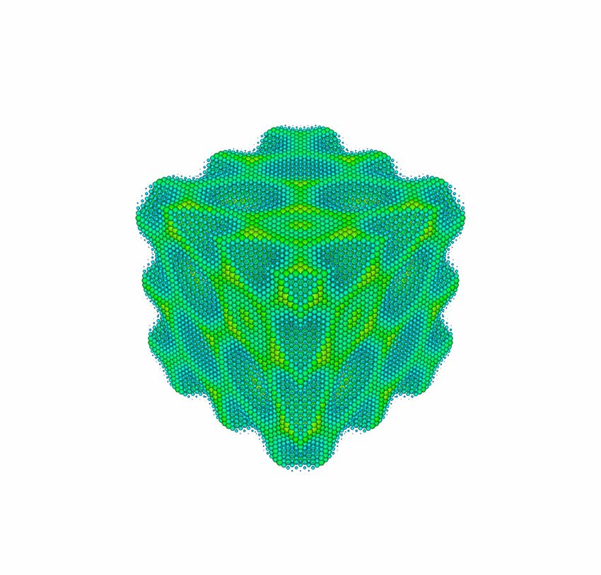
A PREPRINT - A PRIL 14, 2020

space. By explicitly encoding the geometry of materials, ECD is supposed to have high transferability with respect to
different compositions and structures [31]. As ECD captures both geometrical and electronic structural features, 3D
distribution of electronic charge density would have the advantage over classical 1D and 2D descriptors as well as
heterogeneous 3D structural descriptors in terms of the correlation with the electrochemical properties of materials.
Indeed, ECD and its related electronic properties such as the electrostatic potential, electron localization function
and non-covalent interaction index have been used to analyze many materials characteristics, including bonding,
defects, stability,reactivity, and electron, ion and thermal transport [31]. For example, ECD was used to predict 8
materials properties by using the Fourier coefficients of the planar averaged Kohn-Sham charge density fingerprint
features [32]. Abraham et al. [33] calculated 2D charge density to predict the chemical bonding and charge transfer in
magnetic compounds. However both approaches failed to take advantage of the flexibility of the 3D representation [34].
Compared to conventional ML models, 3D CNNs can better link 3D descriptors to the properties efficiently as shown
by [7] (linkage between microstructure and homogenized property) and [9] (linkage between R3DVS and Hartree
energies, testify the invariance to rotation for R3DVS). We believe that the unified representation of ECD makes it
easier to learn unified continuous representation for facilitating downstream prediction tasks by deep convolutional
neural networks [23].
We explored two types of convolutional neural network models for ECD based elastic property prediction. One is
the standard 3D CNNs with two convolutional layers. The other one is a projected 2D CNN models, in which the
ECD matrix is converted to three different image-like representations which are then fed to three 2D CNN networks
whose outputs are then fused together. This allows us to exploit the powerful hierarchical representation capability of
2D CNNs as shown in computer vision [35, 36, 37, 38, 39]. We then conducted extensive benchmark experiments
based on a dataset consisting of 2170 Fcc structured materials and 11 non-redundant datasets generated by leaving
one-element-out at a time.
Our contributions can be summarized as follows:

       • We propose to exploit the ECD descriptor as unified 3D materials representation and combine it with two
         types of 3D CNNs for materials elastic property prediction. We also developed a fusion CNN model based on
         CNN+Magpie and CNN+ECD models.
       • We developed a standard benchmark ECD dataset, named “FCC2170” calculated from 2710 Fcc Structured
         materials from ICSD. This database is characterized by its highly redundant samples with very similar
         compositions. We also developed 11 non-redundant datasets for evaluating the extrapolation capability of
         ECD+CNN models.
       • We performed extensive prediction experiments over the aforementioned datasets using 5-fold cross validation.
         Our results show that our ECD+CNN can be complementary to elemental Magpie feature based models while
         can significantly outperform them over non-redundant datasets, thus demonstrating superior performance on
         some extrapolation experiments.
       • We analyzed the situations when our ECD+CNN models perform better by visually inspecting the distribution
         of test samples and training samples in the 2D space mapped from the learned features.
       • We validated the prediction performance of our models by comparison with DFT-calculated bulk and shear
         modulus for a set of 329 materials of the space group Fm3̄m collected from the Open Quantum Materials
         Database (OQMD) database.

2     Methods
2.1   Datasets

Here we discuss how we create the benchmark datasets for training and validating our proposed method. Due to the high
computational cost to calculate electronic charge density for all the materials in the Materials Project database, we decide
to focus only on materials of one specific space group. First we retrieved 2170 material structures of Fm3̄m space group
(excluding Lanthanides and Actinides) from the Materials Project (MP) database (https://materialsproject.org).
We chose the Fm3̄m structure because its structure is simple and it takes less time to calculate the related elastic properties
using DFT. Most materials of the Fm3̄m space group do not have the charge density or elastic properties available
in the MP database. Hence, we calculated both the electronic charge density [40] and the elastic property [41] using
VASP [42, 43, 44] for the 2,170 samples to form the “FCC2170” dataset . Table 1 lists top 11 elements that are contained
in at least 200 materials of our FCC2070 dataset. Among them, most are from Group 1 (Lithium, Sodium, Potassium,
Rubidium, and Caesium), Group 13 (Indium and Thallium) and Group 17 (Fluorine, Chlorine, and Bromine). The
rest includes Scandium from Group 3. With this dataset, we then use the commonly used cross-validation method to

                                                              3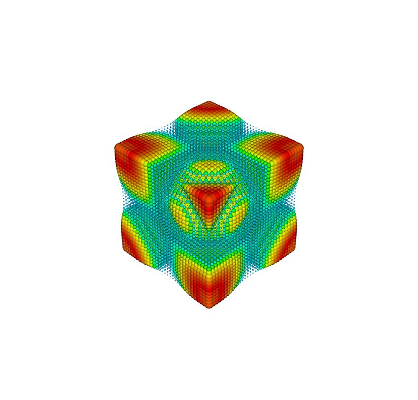
A PREPRINT - A PRIL 14, 2020

evaluate our model’s interpolation performance as done in most machine learning based property prediction studies
[26].
To validate our model’s extrapolation capability, we define a set of leave-one-element-out datasets. For all samples
in FCC2170, we first select those samples containing one specific element E as the test set, and then designate the
remaining samples as the training set. These datasets are called FCC-E-N datasets, where E is the element of interest
and N is the number of training samples without element E. Statistics of all these non-redundant datasets generated
from FCC2170 for elements contained in more than 200 materials are shown in Table 1.

                                    Table 1: Statistics of non-redundant Datasets
    Element            F               K                 Rb              Cs                 Na                 Cl
    dataset       FCC-F-1775      FCC-K-1800 FCC-Rb-1802 FCC-Cs-1814                    FCC-Na-1877       FCC-Cl-1880
 train set size      1755            1800               1802            1814               1877              1880
  test set size       415             370                368             356                293               290
    Element            In              Br                 Li              Sc                 Tl                -
    dataset       FCC-In-1937     FCC-Br-1938 FCC-Li-2148 FCC-Sc-1952                   FCC-Tl-1966            -
 train set size      1937            1938               2148            1952               1966                -
  test set size       233             232                222             218                204                -

2.2   Representations of Materials

We studied and compared two material representations for elastic property prediction including Magpie [8] and
electronic charge density(ECD) [45].

      • Magpie features
        Magpie (Materials-Agnostic Platform for Informatics and Exploration) is an extensive set of features related to
        the constituent elements in materials. The set covers a broad range of physical and chemical properties that
        fall into four different categories: stoichiometric features, elemental property statistics, electronic structure
        features, and ionic compound features [8]. Stoichiometric features only contain the number of elements in
        the compound and their several Lp norms [8]. Elemental property statistics are calculated by computing
        several statistics (e.g., average, minimum, maximum, range and mode) of 22 different elemental properties [8].
        These properties include row and column on the periodic table, average atomic number, the range of atomic
        radii between all elements presenting in compositions, Mendeleev number, atomic weight, covalent radius,
        electro-negativity. Electronic structure features are the average fraction of s, p, d and f valence electrons [18].
        Ionic compound features include the capability of forming an ionic compound (when we assume all elements
        present in a single oxidation state) and two adaptions for calculating the fractions of a compound based on
        electronegativity [46].
      • electronic charge density
        ECD in the form of 3D structural matrix represents the spatial distribution of electronic charge density
        in crystalline materials. It can be calculated by local quantum-mechanical functions related to the Pauli
        exclusion principle [45]. The ab initio method is used to calculate Hartree-Fock wavefunction and the electron
        localization function (ELF) [40]. A single determinant wave function is calculated on a grid in the 3D space
        by hartree Fock or Kohn Sham orbitals ϕi as following:

                                                                    1
                                                      ELF =                                                            (1)
                                                                1 + ( DDh )2
         where
                                                       1X            1 |∆ρ|2
                                                 D=        |∆ϕi |2 −
                                                       2 i           8 ρ
                                                                                                                       (2)
                                                       3
                                                 Dh =    (3π 2 )5/3 ρ5/3
                                                      10
         where ELF has values between 0 and 1, where 1 means the perfect localization. Figure 1 shows the
         visualizations for the ECDs of six representative materials, namely SRCaIn2 , Mn23 C6 , VSiOs2 , RbI, CsBr,
         and Rb2 TeBr6 , where SRCaIn2 , Mn23 C6 , and VSiOs2 possess high bulk modulus. These visualizations
         consist of points that correspond to the values in a material’s ECD matrix. The color and area of each point

                                                            4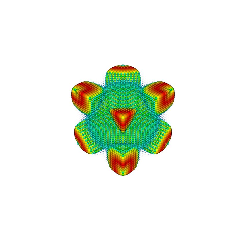
A PREPRINT - A PRIL 14, 2020

         represents the size of each value and together show the distribution of a material’s electron clouds. When the
         value of these points are plotted, we found that points appear in both thick and thin clouds, within the cubes, as
         shown in subfigures 1a, 1b, and 1c. Subfigures 1d, 1e, and 1f show a clear difference from the top-row figures.
         In these figures, there are some empty spaces in the cubes and some dense clusters present in the remaining
         area. These observations correspond to the physical reality that materials with high bulk modulus usually have
         active electrons orbiting across the whole space strongly when compared to materials with lower bulk modulus.
         Among all six materials, we find that although the ECD visualizations share many similar characteristics, there
         are a few distinct differences between them. These minor variations make it possible for us to employ 3D
         CNNs to learn the structural and physical patterns that may characterize the material’s elastic properties.

          (a) SRCaIn2 (32 × 32 × 32)            (b) Mn23 C6 (40 × 40 × 40)            (c) VSiOs2 (24 × 24 × 24)

             (d) RbI (30 × 30 × 30)               (e) CsBr (30 × 30 × 30)             (f) VSiOs2 (48 × 48 × 48)
Figure 1: Visualization of ECD for 6 materials showing clearly contrasting structural features (top and bottom rows).
The top row are materials with high bulk modulus and the bottom row are materials with low bulk modulus. l × w × h
is the actual length, width and height of each ECD matrix.

2.3   Machine Learning Methods

In this work, we use Random Forest and Convolutional Neural Networks (CNNs) with Magpie features as the baseline
methods. We propose that CNNs with ECD can capture certain characteristic relationships between material structures
and their elastic properties.
Random Forest (RF) [47] is a widely used machine learning model in material informatics because of its high accuracy
and robustness [48, 49, 50]. As an ensemble learning algorithm, a RF aggregates the results from different decision
trees (50 in this work). The decision trees are randomly trained based on subsets of training samples and features.
Within a decision tree, a set of decision rules (e.g. Melting temperature > 200.0) is learned by minimizing the variance
of the decision tree. For predicting elastic properties, RF calculates the final results by averaging outputs of all decision
trees.
Convolutional Neural Networks are a type of feed-forward neural network interleaved with convolutional, pooling, and
fully connected layers. It has achieved state-of-the-art(SOTA) performance when applied to computer vision and natural
language processing [36, 39, 51]. The convolutional unit is the core building block of CNNs, which is inspired by the
multi-layered organization of the visual cortex. The unit consists of multiple learnable filters with a given receptive

                                                             5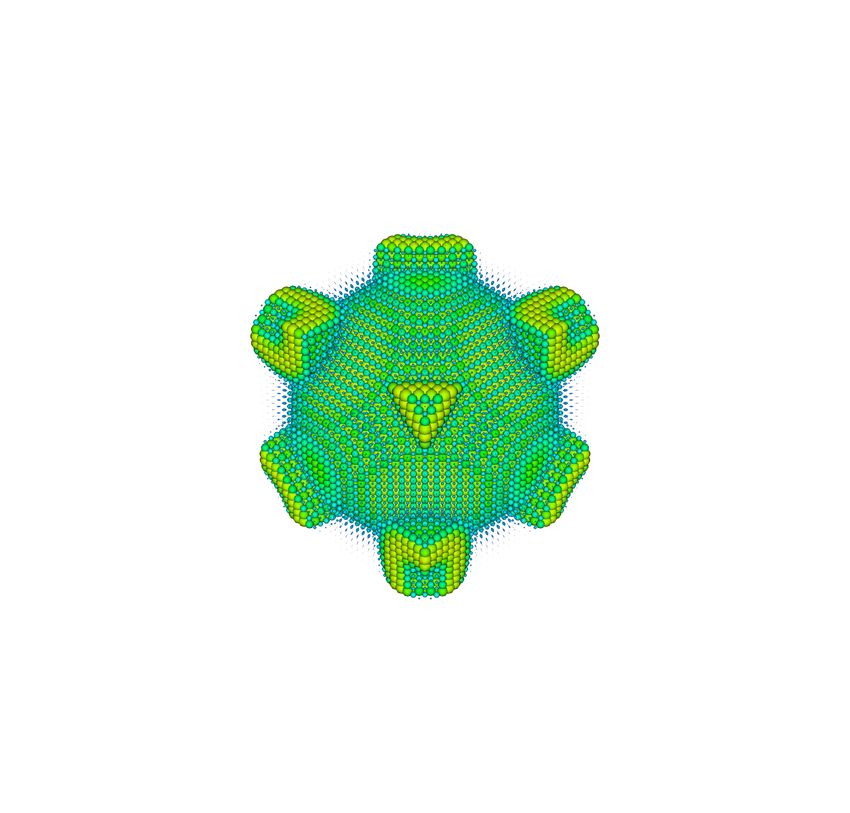
A PREPRINT - A PRIL 14, 2020

field and weight parameters. In our case, the filters are convolved across the full depth of the input volume of the
ECD [52]. The filters are learned hierarchically, where low-level features generate more condensed representations.
                                                                                        0   0   0   0
The computational unit can be constructed by a transformation U = Ftr (X), X ∈ RL ×W ×H ×C , U ∈ RL×W ×H×C .
Ftr denotes the convolutional operation. Let V = [v1 , v2 , . . . , vC ] be the learnable convolutional filters. Then the
outputs of Ftr can be written as U = [u1 , u2 , . . . , uC ], where

                                                                   0
                                                                  C
                                                                  X
                                               u c = vc ∗ X =           vci ∗ xi                                        (3)
                                                                  i=1
                                                          0                          0
Here ∗ denotes the dot product, vc = [vc1 , vc2 , . . . , vcC ], X = [x1 , x2 , . . . , xC ]. We removed the bias terms for
simplicity. vci is a 3D spatial filter convolving on a single channel of X. Stacked outputs of filters produce a 4D tensor
activation map [52]. A pooling layer is used to do non-linear downsampling. It partitions the 3D input into a set of
rectangular boxes. In max-pooling, the pooling layer outputs the maximum value of each sub-region. Then a 3D tensor
is activated through a rectified linear unit (ReLu) [39]. The ReLu operation can be denoted by max(0, P ), where P
is the tensor generated by the max-pooling operation. The same procedure can be applied repeatedly to the whole
activation map. Finally, the output of the convolutional layers is fed to one or more fully connected layers to accomplish
the regression step. Similar procedures are applied in the CNN block in Figure 3.
We implemented two types of convolutional neural networks for learning ECD based features for elastic property
prediction. Figure 2 depicts the 3D CNN architecture in our work. This model has two consecutive convolutional
layers followed by a max pooling layer, and then seven fully connected layers. For simplicity, we did not show the
ReLu [39] activation for all neural layers in Figure 2. The filter size of 2 convolution layers are 5 × 5 × 5 and 4 × 4 × 4,
respectively and the stride has the same size as that of the convolution filters. For all max pooling layers, the sizes of
filters and strides are 2 × 2 × 2. The ECD matrices are fed to the 3D convolutional and pooling layers, and then the
output matrix is flattened and passed to succeeding fully connected layers to calculate final predictions.

Figure 2: The architecture of 3D CNN with ECD representations. The "Scalar" stands for the bulk or shear modulus.
The numbers above each convolutional layers are its parameter settings. For instance, 200@(5 × 5 × 5) means 200
filters with size of 5 × 5 × 5. Unless it is specified, the stride is always the same with the filter size. Two consecutive
convolutional layers are followed by a max-pooling with pooling size and strides both of 2 × 2 × 2. The number below
are outputs of each layer. For fully connected layers, the numbers above them are the number of neurons.

Figure 3 shows the architecture of our 2D CNNs for elastic property prediction. The ECD matrix does not have the
concept of channel as images. Thus, we rotated the ECD matrix so that we can face the cube from x,y,z axes as shown
in different colors of cubes in Figure 3. Then the direction facing to us is considered as the channel direction. To model
the inter-dependencies between channels, we used the Squeeze-and-Excitation (SE) network [53], which can exploit
this inter-dependency by feature recalibration. This model selectively highlights the informative features and suppresses
less useful ones. A SE block is shown in the left corner of Figure 3. In this module, 24 filters of size of 1 × 1 are used
to down-sample the ECD matrix, which was first proposed in [54]. A nonlinearity operation is performed on each pixel
across the channels. After the nonlinear projection, the ECD matrix X of size 60 × 60 × 60 is reduced to the feature
map U of size 60 × 60 × 24. A global average pooling is then used to shrink the feature map into a vector of size 24
along with the dimensions of width and height. Then we use a small set of fully connected layers to transform this
vector into higher level features. The number of neurons on each layers are 4 and 24, respectively. The output s of the
last fully connected layer is reshaped into size of 1 × 1 × 24. The last step is nonlinear excitation and the final output
U 0 of block is achieved by rescaling the U with the activated s:
                                                     U0 = U       σ(s)                                                  (4)

                                                              6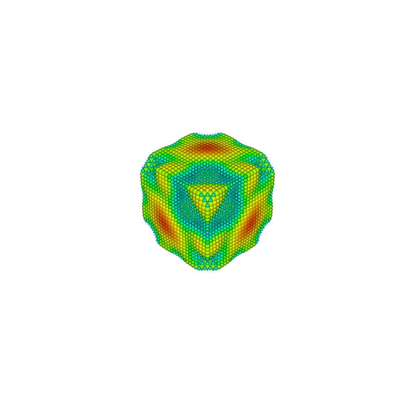
A PREPRINT - A PRIL 14, 2020

where σ is the sigmoid activation function that implements the nonlinear transformation. And           denotes the channel-
wise multiplication between the scalar s and the feature map U 0 .
The SE block in our 2D CNN architecture is followed by CNN blocks. A CNN block has two regular convolutional
layers followed by a max-pooling layer. The first convolution neural has the same filter size and strides of 6 × 6 and
there are 64 filters in this layer. The second CNN layer has a filter size of 5 × 5 and stride of 2 × 2 and there are 128
filters in total. All max-pooling layers have the same pooling size and strides of 2 × 2, respectively.
For each of the projection map of x, y, and z, there is a SE and CNN block for feature extraction. The outputs of them
are concatenated into a vector of size 384. Six fully connected layers are then used to map this learned features into
elastic property values. The number of neurons on these fully connected layer are 4096, 4096, 128, 128, 128 and 32
respectively.

Figure 3: The architecture of the 2D CNN with ECD representation. The "Scalar" stands for the bulk or shear modulus.
The model includes three parts: mainframe, SE block and CNN block. In the mainframe, we have three branches
whose outputs are concatenated and fed into six fully connected layers. The numbers above each component/layer are
the number of neurons of that layer. In SE block, the labels of R and S are reshape and channel-wise multiplication
operations. For simplicity, we ignore the max-pooling layers following every convolutional layer in the CNN block.
Numbers below each component are the output dimension of that layer.

For the baseline algorithm, we also train a 2D CNN model with the Magpie features. To do that, we append 12 zeros to
the Magpie features to get a vector of 1x144, which is then reshaped into a 2D matrix of size 12 × 12. The CNN model
for Magpie features has two consecutive convolutional layers followed by an average pooling layer. Then an additional
convolutional layer is added followed by two fully connected layers. The model parameters are set as follows: the
kernel size and strides of the first convolutional layer are 3x3 and 1x1 and the number of filters is 32; the kernel size and
strides of the second convolutional layer are 3x3 and 1x1 and the number of filters is 48; the pooling size and strides of
the average pooling layer are both set as 2x2; the kernel size and strides of the third convolutional layer are 3x3 and 1x1
and the number of filters is 64; the number of neurons of the two fully connected layers are 48 and 32, respectively.

2.4   Training and Implementation

Figure 2 shows the detailed architecture of our 3D CNN and its parameters. The models are implemented using
the open-source libraries of TensorFlow (https://www.tensorflow.org) and Keras (https://keras.io). The
performance of the models are evaluated using 5-fold cross validation. The input ECD has a shape of 60 × 60 × 60 by
interpolation for smaller matrices. The CNN for Magpie is also trained using the Adam optimizer [55] with a batch
size of 32 and learning rate of 0.001. The 3D CNN model parameters are learned using the Adam optimizer [55]
with a initial learning rate of 0.0005. For the 2D CNNs with ECD, we use the SGD optimizer to learn the model
                                                                     epoch
parameters. The initial learning rate is 0.001 and it drops by 0.5b 10 c , where epoch is the current epoch. The

                                                             7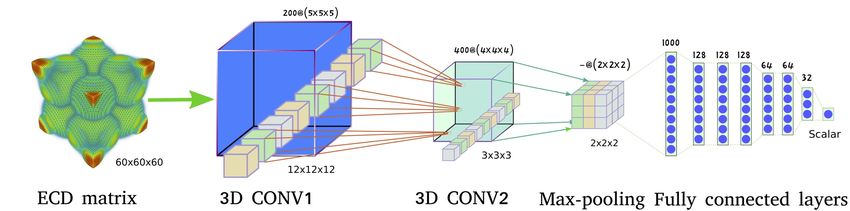
A PREPRINT - A PRIL 14, 2020

mean absolute error (MAE) is used as the loss function for all three CNN models. The open source matminer
(https://hackingmaterials.lbl.gov/matminer/) is utilized to calculate the Magpie features.

3     Results and Discussions
In this section, we discuss the experiments demonstrating the potential of ECD for material representation and elastic
property prediction. The experiments are separated into two parts in terms of the evaluation approaches: experiments
with 5-fold cross validation and experiments focusing on extrapolation performance evaluation. All experiments of
CNN models are repeated 5 times and the result presented herein is the average of their outputs.

3.1    5-fold cross validation experiments with redundant dataset

Table 2 shows the results from 5-fold cross validation on the whole dataset with 2170 samples. We find that the baseline
models using Magpie features are better than CNNs with ECD across all evaluation metrics for predicting bulk and
shear moduli. Overall, RF with Magpie performs slightly better than CNNs with Magpie. Although R2 of RF with
Magpie is 0.001 lower than that of CNNs with Magpie in predicting bulk modulus, RF with Magpie achieves much
better results in predicting shear modulus (R2 is 0.049 higher). Similar observations apply to performance evaluated in
terms of Root Mean Square Error (RMSE). This better performance of Magpie based RF models are not unexpected.
First, all samples in this FCC2170 dataset belong to the Fm3̄m space group. By sharing similar structures, the Magpie
features are able to capture most of the elastic property variation due to composition difference. The high structural
similarity of the dataset helps the baseline methods based on composition Magpie features predict the elastic properties
well. Another reason is that the FCC2170 contains many similar samples in terms of compositions. The high redundant
samples also makes the baseline models with Magpie features to make precise predictions by exploiting redundant
neighbor samples in the training set when evaluated on the test set during cross-validation. However, the machine
learning models trained with redundant training set can lead to low extrapolation performance as shown in our previous
study [56].
Here we show that ECD can be used as a complementary materials descriptor for elastic property prediction together
with the Magpie features. To verify this, We pre-trained a CNN model with Magpie features and a 2D CNN model with
ECD. Then we fused these two models by concatenating the outputs of the penultimate layers of these two models to
generate a output latent feature vector of dimension 64, which is then fed to three fully connected layers with 128, 64,
and 32 neurons respectively. The Adam optimizer [55] is used for training with a learning rate of 0.001. This fusion
neural network model with mixed Magpie and ECD descriptor yielded the best R2 and RMSE of 0.955 (0.804) and
16.530 (15.780) in predicting bulk (shear) modulus respectively as shown in Table 2 . This confirms that ECD and
Magpie can work together to achieve better performance for elastic property prediction. In addition, our experiments
also showed that the projected 2D CNN achieved significantly better performance than the basic 3D CNN models. The
R2 and RMSE of 2D-CNN with ECD are 0.912 and 23.401 in predicting bulk modulus compared to 0.884 and 26.819
of 3D-CNNs with ECD. The R2 and RMSE of 2D CNN with ECD are 0.768 and 17.192 in predicting shear modulus
compared to 0.745 and 17.944 of 3D-CNNs with ECD.

      Table 2: Performance Comparisons of models with Magpie and ECD descriptors using 5-fold cross validation
                     RF+Magpie      CNN+Magpie 3D-CNN+ECD 2D CNN+ECD                        Fusion
            Type
                     R2    RMSE     R2     RMSE       R2     RMSE     R2     RMSE        R2      RMSE
            bulk 0.943 18.721 0.944 18.423 0.884 26.819 0.912 23.401 0.955 16.530
           shear 0.794 16.142 0.745 17.959 0.745 17.944 0.768 17.192 0.804 15.780

3.2    Extrapolation Experiments with non-redundant datasets

ML models with elemental descriptors such as Magpie can achieve good cross-validation performance for datasets
consisting of redundant (computationally very similar samples) such as FCC2170. However, the better performance of
the fusion model with CNN with Magpie and 2D-CNN with ECD implies that for the ECD descriptor can help to make
better predictions over a certain subset of test samples. In this section, we aim to construct non-redundant dataset and
show that our CNN models with the ECD descriptor can achieve better performance on non-redundant datasets or for
test samples with few highly similar neighbor samples.
For these extrapolation experiments, we trained and tested the prediction models over the FCC-E-N datasets as described
in Section 2.1. The performance comparison results of the extrapolation experiments for bulk and shear modulus
prediction are shown in Table 3. There are 22 sets of experiments with 11 of them for predicting bulk modulus and the

                                                           8
A PREPRINT - A PRIL 14, 2020

other 11 for predicting shear modulus by five different algorithms including RF+Magpie, CNN+Magpie, 3D-CNN+ECD,
2D-CNN+ECD, and the latest crystal graph convolutional neural network (CGCNN) [25], which also uses structural
information. We highlighted the best performance scores for each experiments and count how many experiments each
algorithm achieved the best scores. As shown in Table 3, the RF with Magpie and CNN with Magpie worked the best
for 5 and 6 experiments respectively. However, impressively, for these non-redundant training/testing experiments, our
ECD descriptor based 3D-CNN-ECD and 2D-CNN-ECD outperformed the others for 4 and 5 experiments respectively,
which reflecting the importance of the structure based ECD descriptor for elastic property prediction. In contrast, the
popular CGCNN only achieved the best performance out of 2 experiments, which demonstrated the advantage of our
ECD based atomic structure representation.

       Table 3: Extrapolation prediction performance comparison on non-redundant leave-one-element-out datasets
                        RF+Magpie          CNN+Magpie      3D-CNN+ECD        2D-CNN+ECD            CGCNN
      Elem Type
                        R2      RMSE       R2     RMSE       R2     RMSE      R2      RMSE      R2      RMSE
               bulk -0.529 26.797 -0.809 29.102 -0.051 22.212 -0.448 26.080 -2.217 35.554
        F
              shear -3.350 18.117 -6.912 24.315 -1.202 12.878 -1.293 13.151 -0.548 10.657
               bulk   0.776     6.067     0.646    7.573   0.510    8.969    0.570     8.397   0.474     9.055
        K
              shear 0.810       2.641     0.548    4.014   0.389    4.733    0.367     4.817   0.146     5.523
               bulk   0.867     4.603     0.869    4.579   0.753    6.287    0.777     5.966   0.275 10.290
       Rb
              shear 0.778       2.767     0.727    3.064   0.608    3.657    0.719     3.111   0.268     4.944
               bulk -0.128 11.232 0.760            5.166   0.448    7.818    0.067 10.158 -0.144 10.934
       Cs
              shear -4.327 11.199 0.492            3.446   0.014    4.743 -1.137 7.083         0.344     3.881
               bulk   0.630 16.398 0.833 11.013 0.660 15.708 0.616 16.689 0.605 16.223
       Na
              shear 0.545       8.366     0.386    9.716   0.548    8.340    0.451     9.196   0.351     9.863
               bulk   0.410 15.935 0.529 14.151 0.591 13.009 0.716                     11.05   0.534 13.119
       Cl
              shear -0.477 10.715 0.213            7.765   0.339    7.160    0.093     8.394 -0.197 9.366
               bulk   0.829 20.780 0.780 23.550 0.725 26.326 0.773 23.908 0.761 24.460
       In
              shear 0.791       8.250     0.771    8.618   0.683 10.136 0.793          8.207   0.655 10.416
               bulk   0.921     4.464     0.923    4.585   0.912    4.700    0.923     4.411   0.631     9.245
       Br
              shear 0.630       2.290 -0.078 3.857         0.755    1.861    0.824     1.579 -2.661 6.975
               bulk   0.418 29.869 0.867 14.253 0.519 27.142 0.454 28.937 0.732 20.121
       Li
              shear -0.232 17.799 0.416 12.239 0.428 12.126 0.451 11.881 0.388 12.488
               bulk   0.855 23.276 0.908 18.538 0.756 30.195 0.850 23.688 0.818 25.983
       Sc
              shear 0.781 12.996 0.707 15.024 0.682 15.650 0.635 16.786 0.667 16.007
               bulk -0.370 24.574 0.421 15.973 0.219 18.529 0.501 14.833 0.550 14.040
       Tl
              shear 0.456       6.745     0.437    6.815   0.559    6.068    0.557     6.084   0.427     6.818
      # of the best           5                 6                 4                 5                 2

3.3     Visualization Study of when ECD descriptor works better

To understand on why our ECD based CNN models worked better than Magpie features on some datasets but not others,
we conducted a visualization study for all the extrapolation experiments. For magpie features, we directly apply the
t-distributed Stochastic Neighbor Embedding (t-SNE) [57] to the dataset. For the ECD based features, directly applying
t-SNE is not feasible due to the memory limit. So we first applied max-pooling to the 3D ECD matrices with strides
of (6, 6, 6) and pooling size of (6, 6, 6) before feeding them into t-SNE. Hence the final size of the ECD matrices is
(10, 10, 10), which are then flattened to a 1D vector of 1,000 elements. Then we applied t-SNE to this 1D vector to
reduce the dimension to 2.

                                                          9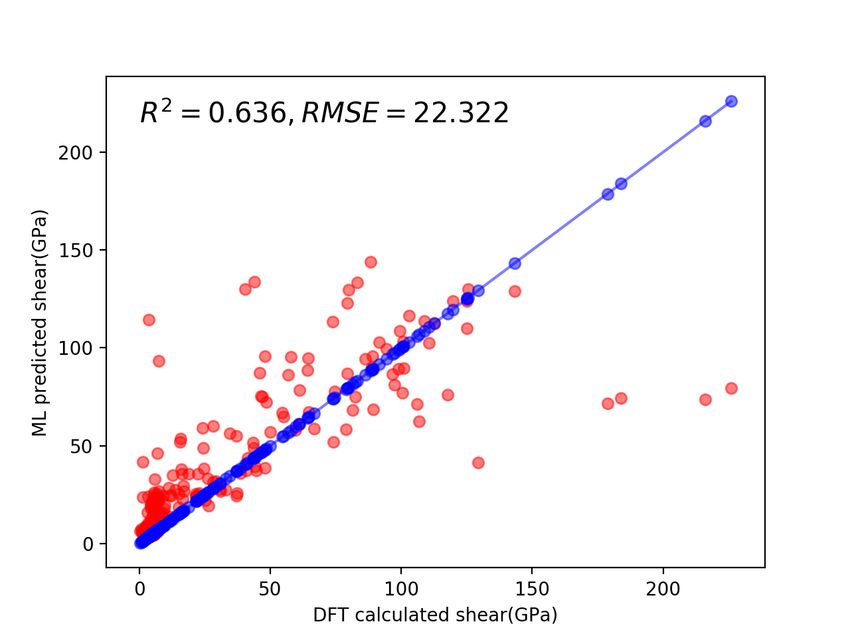
A PREPRINT - A PRIL 14, 2020

          (a) 2D map of Magpie features for FCC-Cl-1880                (b) 2D map of ECD features for FCC-Cl-1880

          (c) 2D map of Magpie features for FCC-Tl-1966                 (d) 2D map of ECD features for FCC-Tl-1966
Figure 4: Visualization of high-dimensional features for element Chlorine and Thallium by t-SNE. Blue dots are training data and
red dots are test data.

Figure 4 shows 2D visualization of the high-dimension Magpie and ECD features for two datasets: FCC-Chlorine-1880
and FCC-Thallium-1966 over which the ECD based models outperform Magpie feature based models. The training
samples are labelled as blue points while the test samples are red points. First, Figure 4 (a) and (b) show the distribution
of training and test samples with Magpie features and with ECD features respectively for the FCC-Chlorine-1880
dataset. In subfigure 4a, we found that there exist three large clusters of test samples (red points) that have few similar
training samples around. This corresponds to the low prediction performance for Magpie based models. The best
performance for both bulk and shear modulus prediction is achieved by CNN+Magpie with R2 of 0.529 and 0.213
respectively. In contrast, subfigure 4b shows the 2D distribution of the samples represented with ECD features. It can be
found that the test samples are mostly mixed with training samples, leading to much better prediction performance: the
best performance for bulk modulus prediction is achieved by 2D-CNN+ECD with R2 of 0.716, which is significantly

                                                              10
A PREPRINT - A PRIL 14, 2020
better (35%)than 0.529, the best prediction performance achieved by Magpie based models. The best performance for
shear prediction is achieved by 3D-CNN+ECD with R2 of 0.339, which is also 59% better than 0.213, the best R2 score
of Magpie based models.
Figure 4 (c) and (d) show the distribution of training and test samples with Magpie features and with ECD features
respectively for the FCC-Thallium-1966 dataset. In subfigure 4c, we found that clusters of test samples (red points)
are closer to training samples compared to subfigure 4a. There is no large clusters of isolated test samples. The best
performance for bulk modulus is achieved by CNN+Magpie with R2 of 0.421. The best performance for shear modulus
prediction is achieved by RF+Magpie with R2 of 0.456. In contrast, subfigure 4d shows the 2D distribution of the
samples represented with ECD features. It can be found that the test samples are better mixed with training samples
than subfigure 4a, leading to better prediction performance. The best performance for both bulk modulus prediction
is achieved by 2D-CNN+ECD with R2 of 0.501 and the best shear modulus prediction performance is achieved by
3D-CNN+ECD with R2 of 0.559. In this dataset, the best ECD based model is (0.559-0.421)/0.421 = 19% better than
the best Magpie based model for bulk modulus prediction. The performance gap is much smaller compared to that
(35%) on the FCC-Chlorine-1880 dataset. The best ECD based model is also (0.559-0.456)/0.456 = 24.9% better than
the best Magpie based model for shear modulus prediction, which is however much smaller than the performance gap
over the FCC-Chlorine-1880 dataset, which is 59%. These findings can partially explain why ECD based models are
superior to Magpie based models in predicting elastic properties for these two datasets. It shows the structure based
ECD descriptor can be a complementary descriptor to elemental Magpie features for elastic property prediction due to
their better neighborhood structure of the samples. This analysis is consistent to those observation that neighbor sample
distribution significantly affects the performance of neural network based prediction models [58].
3.4 DFT validation
To further validate our neural network models, we predict the bulk and shear modulus of a set of external materials from
the OQMD [59] database and compared them to DFT calculated ones. We first collect all the materials of the space
group Fm3̄m from OQMD and then remove the duplicates existing in the Material Project database that we used as the
training set. We also filter out the materials having more than 40 atoms in the unit cell. We finally obtain 329 materials
as our test set. Then we apply the trained fusion model (Magpie + ECD features) trained with Material Project samples
to predict the bulk and shear modulus of the 329 samples in the test set and compared them with DFT-calculated ones
as shown in Figure 5. We find that our fusion model successfully predicted the bulk modulus for the 329 materials with
good alignment with DFT calculated values. The R2 and RMSE in predicting bulk are 0.93 and 21.331 as shown in
Figure 5a. However, we also find that the ML-predicted the predicted shear modulus values deviate much more from
the DFT calculated ones compared to the bulk modulus, which reflects the fact that it is more difficult to predict shear
modulus than bulk modulus. We also observe that most of the deviations of the predicted values compared with DFT
calculated ones are from the regions with low bulk or shear modulus and the predicted values usually are large than the
DFT calculated ones.
(a) (b)
Figure 5: Panels (a) and (b) show ML-predicted versus DFT-calculated bulk and shear modulus respectively.
11A PREPRINT - A PRIL 14, 2020
4 Conclusions
We propose to combine deep convolutional neural networks and electronic charge density (ECD) for materials elasticity
prediction. We demonstrate that the ECD descriptor can be used to predict bulk and shear modulus with CNNs model.
We created a benchmark dataset named “FCC2170” with 2,170 materials of Fm3̄m space group from Materials Project
database and derived 11 non-redundant leave-one-element-out datasets for benchmarking the proposed ML models
with ECD and elemental Magpie features. Our computational experiments showed that due to the structural similarity
among the samples of the FCC2170 dataset, the elemental Magpie feature with CNN models achieved the best results,
which however, can be enhanced by the fusion models with both Magpie and ECD features. In addition, our benchmark
studies on the non-redundant datasets showed that the structure-based ECD feature with CNNs can achieve better
extrapolation prediction performances over half prediction tasks out of the total 22 experiments for prediction bulk and
shear modulus.
To further understand the power of the ECD descriptor, we visualized the distribution of training and test datasets of
two descriptor types using t-SNE. It shows that when the training set and testing set of the non-redundant datasets
have higher level of mixing, the Magpie-based CNN models work better. When they have lower level of mixing, the
ECD descriptor based models significantly outperform the Magpie based CNN models. The results demonstrate the
importance of structure based features for achieving higher extrapolation and generalization prediction capability. It is
expected that our ECD descriptor with CNN models can also be applied to a variety of problems in material science,
especially with the development of algorithms for predicting ECD [31]. Currently, we are generating more ECD dataset
with more space groups to extend this method to more materials with diverse structures.
5 Author contribution
Conceptualization, M.H. and J.H.; methodology, Y.Z. and J.H.; software, Y.Z.; validation, Y.Z.; data curation, Y.L.;
writing–original draft preparation, Y.Z., J.H., and M.H.; writing–review and editing, Y.Z., J.H., M.H., and S.L.;
visualization, Y.Z.; supervision, J.H.; project administration, J.H. and M.H.; funding acquisition, J.H. and M.H.
6 Funding
This research was partially funded by NSF under grant number 1940099,1905775,and OIA-1655740 and DOE under
grant number de-sc0020272.
References
[1] Zhuo Cao, Yabo Dan, Zheng Xiong, Chengcheng Niu, Xiang Li, Songrong Qian, and Jianjun Hu. Convolutional
neural networks for crystal material property prediction using hybrid orbital-field matrix and magpie descriptors.
Crystals, 9(4):191, 2019.
[2] Bart Olsthoorn, R Matthias Geilhufe, Stanislav S Borysov, and Alexander V Balatsky. Band gap prediction for
large organic crystal structures with machine learning. Advanced Quantum Technologies, 2(7-8):1900023, 2019.
[3] Austin D Sendek, Ekin D Cubuk, Evan R Antoniuk, Gowoon Cheon, Yi Cui, and Evan J Reed. Machine
learning-assisted discovery of solid li-ion conducting materials. Chemistry of Materials, 31(2):342–352, 2018.
[4] Patrick Avery, Xiaoyu Wang, Corey Oses, Eric Gossett, Davide M Proserpio, Cormac Toher, Stefano Curtarolo,
and Eva Zurek. Predicting superhard materials via a machine learning informed evolutionary structure search. npj
Computational Materials, 5(1):1–11, 2019.
[5] Ekin D Cubuk, Austin D Sendek, and Evan J Reed. Screening billions of candidates for solid lithium-ion
conductors: A transfer learning approach for small data. The Journal of chemical physics, 150(21):214701, 2019.
[6] Lihua Chen, Huan Tran, Rohit Batra, Chiho Kim, and Rampi Ramprasad. Machine learning models for the lattice
thermal conductivity prediction of inorganic materials. Computational Materials Science, 170:109155, 2019.
[7] Ahmet Cecen, Hanjun Dai, Yuksel C Yabansu, Surya R Kalidindi, and Le Song. Material structure-property
linkages using three-dimensional convolutional neural networks. Acta Materialia, 146:76–84, 2018.
[8] Logan Ward, Ankit Agrawal, Alok Choudhary, and Christopher Wolverton. A general-purpose machine learning
framework for predicting properties of inorganic materials. npj Computational Materials, 2:16028, 2016.
12A PREPRINT - A PRIL 14, 2020
[9] Seiji Kajita, Nobuko Ohba, Ryosuke Jinnouchi, and Ryoji Asahi. A universal 3d voxel descriptor for solid-state
material informatics with deep convolutional neural networks. Scientific reports, 7(1):16991, 2017.
[10] Sandip De, Albert P Bartók, Gábor Csányi, and Michele Ceriotti. Comparing molecules and solids across structural
and alchemical space. Physical Chemistry Chemical Physics, 18(20):13754–13769, 2016.
[11] Matthias Rupp, Alexandre Tkatchenko, Klaus-Robert Müller, and O Anatole Von Lilienfeld. Fast and accurate
modeling of molecular atomization energies with machine learning. Physical review letters, 108(5):058301, 2012.
[12] P Villars, K Cenzual, J Daams, Y Chen, and S Iwata. Data-driven atomic environment prediction for binaries
using the mendeleev number: Part 1. composition ab. Journal of alloys and compounds, 367(1-2):167–175, 2004.
[13] Felix Faber, Alexander Lindmaa, O Anatole von Lilienfeld, and Rickard Armiento. Crystal structure repre-
sentations for machine learning models of formation energies. International Journal of Quantum Chemistry,
115(16):1094–1101, 2015.
[14] Matthias Rupp. Machine learning for quantum mechanics in a nutshell. International Journal of Quantum
Chemistry, 115(16):1058–1073, 2015.
[15] Albert P Bartók, Risi Kondor, and Gábor Csányi. On representing chemical environments. Physical Review B,
87(18):184115, 2013.
[16] Wojciech J Szlachta, Albert P Bartók, and Gábor Csányi. Accuracy and transferability of gaussian approximation
potential models for tungsten. Physical Review B, 90(10):104108, 2014.
[17] Luca M Ghiringhelli, Jan Vybiral, Sergey V Levchenko, Claudia Draxl, and Matthias Scheffler. Big data of
materials science: critical role of the descriptor. Physical review letters, 114(10):105503, 2015.
[18] Bryce Meredig, Ankit Agrawal, Scott Kirklin, James E Saal, JW Doak, Alan Thompson, Kunpeng Zhang, Alok
Choudhary, and Christopher Wolverton. Combinatorial screening for new materials in unconstrained composition
space with machine learning. Physical Review B, 89(9):094104, 2014.
[19] Tien Lam Pham, Hiori Kino, Kiyoyuki Terakura, Takashi Miyake, Koji Tsuda, Ichigaku Takigawa, and Hieu Chi
Dam. Machine learning reveals orbital interaction in materials. Science and technology of advanced materials,
18(1):756, 2017.
[20] Logan Ward, Alexander Dunn, Alireza Faghaninia, Nils ER Zimmermann, Saurabh Bajaj, Qi Wang, Joseph
Montoya, Jiming Chen, Kyle Bystrom, Maxwell Dylla, et al. Matminer: An open source toolkit for materials data
mining. Computational Materials Science, 152:60–69, 2018.
[21] Ya Zhuo, Aria Mansouri Tehrani, and Jakoah Brgoch. Predicting the band gaps of inorganic solids by machine
learning. The journal of physical chemistry letters, 9(7):1668–1673, 2018.
[22] Dipendra Jha, Kamal Choudhary, Francesca Tavazza, Wei-keng Liao, Alok Choudhary, Carelyn Campbell, and
Ankit Agrawal. Enhancing materials property prediction by leveraging computational and experimental data using
deep transfer learning. Nature communications, 10(1):1–12, 2019.
[23] Juhwan Noh, Jaehoon Kim, Helge S Stein, Benjamin Sanchez-Lengeling, John M Gregoire, Alan Aspuru-Guzik,
and Yousung Jung. Inverse design of solid-state materials via a continuous representation. Matter, 2019.
[24] Michael J Willatt, Félix Musil, and Michele Ceriotti. Atom-density representations for machine learning. The
Journal of chemical physics, 150(15):154110, 2019.
[25] Tian Xie and Jeffrey C Grossman. Crystal graph convolutional neural networks for an accurate and interpretable
prediction of material properties. Physical review letters, 120(14):145301, 2018.
[26] Chi Chen, Weike Ye, Yunxing Zuo, Chen Zheng, and Shyue Ping Ong. Graph networks as a universal machine
learning framework for molecules and crystals. Chemistry of Materials, 31(9):3564–3572, 2019.
[27] Graeme Henkelman, Andri Arnaldsson, and Hannes Jónsson. A fast and robust algorithm for bader decomposition
of charge density. Computational Materials Science, 36(3):354–360, 2006.
[28] Tao Ouyang and Ming Hu. Competing mechanism driving diverse pressure dependence of thermal conductivity of
x te (x= hg, cd, and zn). Physical Review B, 92(23):235204, 2015.
[29] Guangzhao Qin, Zhenzhen Qin, Sheng-Ying Yue, Qing-Bo Yan, and Ming Hu. External electric field driving the
ultra-low thermal conductivity of silicene. Nanoscale, 9(21):7227–7234, 2017.
[30] Guangzhao Qin, Zhenzhen Qin, Huimin Wang, and Ming Hu. Lone-pair electrons induced anomalous enhancement
of thermal transport in strained planar two-dimensional materials. Nano Energy, 50:425–430, 2018.
[31] Sheng Gong, Tian Xie, Taishan Zhu, Shuo Wang, Eric R Fadel, Yawei Li, and Jeffrey C Grossman. Predicting
charge density distribution of materials using a local-environment-based graph convolutional network. Physical
Review B, 100(18):184103, 2019.
13A PREPRINT - A PRIL 14, 2020
[32] Ghanshyam Pilania, Chenchen Wang, Xun Jiang, Sanguthevar Rajasekaran, and Ramamurthy Ramprasad. Accel-
erating materials property predictions using machine learning. Scientific reports, 3:2810, 2013.
[33] Jisha Annie Abraham, Gitanjali Pagare, and Sankar P Sanyal. Electronic structure, electronic charge density, and
optical properties analysis of gdx3 (x= in, sn, tl, and pb) compounds: dft calculations. Indian Journal of Materials
Science, 2015, 2015.
[34] Hwanho Choi, Kee-Sun Sohn, Myoungho Pyo, Kee-Choo Chung, and Hwangseo Park. Predicting the electro-
chemical properties of lithium-ion battery electrode materials with the quantum neural network algorithm. The
Journal of Physical Chemistry C, 123(8):4682–4690, 2019.
[35] Xiaozhi Chen, Huimin Ma, Ji Wan, Bo Li, and Tian Xia. Multi-view 3d object detection network for autonomous
driving. In Proceedings of the IEEE Conference on Computer Vision and Pattern Recognition, pages 1907–1915,
2017.
[36] Karen Simonyan and Andrew Zisserman. Very deep convolutional networks for large-scale image recognition.
arXiv preprint arXiv:1409.1556, 2014.
[37] Daniel Maturana and Sebastian Scherer. Voxnet: A 3d convolutional neural network for real-time object
recognition. In 2015 IEEE/RSJ International Conference on Intelligent Robots and Systems (IROS), pages
922–928. IEEE, 2015.
[38] Christian Szegedy, Sergey Ioffe, Vincent Vanhoucke, and Alexander A Alemi. Inception-v4, inception-resnet and
the impact of residual connections on learning. In Thirty-First AAAI Conference on Artificial Intelligence, 2017.
[39] Alex Krizhevsky, Ilya Sutskever, and Geoffrey E Hinton. Imagenet classification with deep convolutional neural
networks. In Advances in neural information processing systems, pages 1097–1105, 2012.
[40] Kurt Artmann. Berechnung der seitenversetzung des totalreflektierten strahles. Annalen der Physik, 437(1-2):87–
102, 1948.
[41] Zhi-jian Wu, Er-jun Zhao, Hong-ping Xiang, Xian-feng Hao, Xiao-juan Liu, and Jian Meng. Crystal structures
and elastic properties of superhard ir n 2 and ir n 3 from first principles. Physical Review B, 76(5):054115, 2007.
[42] Georg Kresse and Jürgen Hafner. Ab initio molecular dynamics for liquid metals. Physical Review B, 47(1):558,
1993.
[43] Georg Kresse and Jürgen Furthmüller. Efficiency of ab-initio total energy calculations for metals and semiconduc-
tors using a plane-wave basis set. Computational materials science, 6(1):15–50, 1996.
[44] Georg Kresse and Jürgen Furthmüller. Efficient iterative schemes for ab initio total-energy calculations using a
plane-wave basis set. Physical review B, 54(16):11169, 1996.
[45] Bernard Silvi and Andreas Savin. Classification of chemical bonds based on topological analysis of electron
localization functions. Nature, 371(6499):683, 1994.
[46] William D Callister, David G Rethwisch, et al. Materials science and engineering: an introduction, volume 7.
John Wiley & Sons New York, 2007.
[47] Leo Breiman. Random forests. Machine learning, 45(1):5–32, 2001.
[48] Keisuke Takahashi and Lauren Takahashi. Creating machine learning-driven material recipes based on crystal
structure. The journal of physical chemistry letters, 10(2):283–288, 2019.
[49] Felipe Oviedo, Zekun Ren, Shijing Sun, Charlie Settens, Zhe Liu, Noor Titan Putri Hartono, Ramasamy Savitha,
Brian L DeCost, Siyu IP Tian, Giuseppe Romano, et al. Fast classification of small x-ray diffraction datasets using
data augmentation and deep neural networks. arXiv preprint arXiv:1811.08425, 2018.
[50] Logan Ward, Ruoqian Liu, Amar Krishna, Vinay I Hegde, Ankit Agrawal, Alok Choudhary, and Chris Wolverton.
Including crystal structure attributes in machine learning models of formation energies via voronoi tessellations.
Physical Review B, 96(2):024104, 2017.
[51] Yoon Kim. Convolutional neural networks for sentence classification. arXiv preprint arXiv:1408.5882, 2014.
[52] Yann LeCun, Léon Bottou, Yoshua Bengio, Patrick Haffner, et al. Gradient-based learning applied to document
recognition. Proceedings of the IEEE, 86(11):2278–2324, 1998.
[53] Jie Hu, Li Shen, and Gang Sun. Squeeze-and-excitation networks. In Proceedings of the IEEE conference on
computer vision and pattern recognition, pages 7132–7141, 2018.
[54] Min Lin, Qiang Chen, and Shuicheng Yan. Network in network. arXiv preprint arXiv:1312.4400, 2013.
[55] Diederik P Kingma and Jimmy Ba. Adam: A method for stochastic optimization. arXiv preprint arXiv:1412.6980,
2014.
14A PREPRINT - A PRIL 14, 2020
[56] Zheng Xiong, Yuxin Cui, Zhonghao Liu, Yong Zhao, Ming Hu, and Jianjun Hu. Evaluating explorative prediction
power of machine learning algorithms for materials discovery using k-fold forward cross-validation. Computational
Materials Science, 171:109203, 2020.
[57] Laurens van der Maaten and Geoffrey Hinton. Visualizing data using t-sne. Journal of machine learning research,
9(Nov):2579–2605, 2008.
[58] Jon Paul Janet, Chenru Duan, Tzuhsiung Yang, Aditya Nandy, and Heather J Kulik. A quantitative uncertainty
metric controls error in neural network-driven chemical discovery. Chemical Science, 2019.
[59] James E Saal, Scott Kirklin, Muratahan Aykol, Bryce Meredig, and Christopher Wolverton. Materials design and
discovery with high-throughput density functional theory: the open quantum materials database (oqmd). Jom,
65(11):1501–1509, 2013.
15You can also read