Predicting the Resale Price of HDB Flats in Singapore - 熊可欣 ...
←
→
Page content transcription
If your browser does not render page correctly, please read the page content below
Predicting the Resale Price of HDB Flats in
                           Singapore
                                        *
                                            Final Project of NUS CS5228-2020/2021 (Semester 2)

                                                                Team 5

                    Xiong Kexin                               Yao Yihang                              Liu Xing
                    A0196551X                                A0209966M                               A0225169B
                e0389037@u.nus.edu                        e0454417@u.nus.edu                     e0575803@u.nus.edu

   Abstract—Based on the properties of HDB flats in Singapore,        B. Goals
the resale price can be predicted by data mining methods. This
report will show how we did implement the knowledge we learnt            Our project aims at predicting the resale price of an HDB
through CS5228 course, practice EDA, data preprocessing and           flat based on its properties, including size, number of rooms,
model training and complete the prediction of the resale price        type, model, location, nearby amenities and its so on. Since it
of HDB flats in Singapore.
   Index Terms—price prediction, knowledge discovery, data            is obviously a regression task, we plan to use different regres-
mining, regression task.                                              sion techniques to do this prediction and compare their results.
                                                                      In addition, other results such as the importance of different
                       I. I NTRODUCTION                               attributes, error analysis, and other necessary discussion will
                                                                      be included.
  The resale market of HDB flats is big business in Singapore.
To find a good prices as either a buyer or a seller, it is
important to have good understanding of what affects the              III. E XPLORATORY DATA A NALYSIS AND P REPROCESSING
market value of a HDB flat. The goal of this project is to
predict the resale price of a HDB flat based on its properties.       A. Exploratory Data Analysis
To make better prediction, exploratory data analysis and data
                                                                         Exploratory Data Analysis is a process of performing in-
preprocessing, feature engineering and model selection is
                                                                      vestigations on datasets so as to gain initial impressions, to
implemented.
                                                                      discover patterns, to spot anomalies and to get summary statics
                II. M OTIVATION AND G OALS                            and visualisations.
                                                                         In good practice to understand the data and get insights
A. Motivation                                                         from it, we first loaded the datasets and did Exploratory Data
   The majority of the residential housing in Singapore are           Analysis on it. By using ”head()” function of pandas library,
HDB flats, which are home to approximately 78.7% of the               we can see the raw data structure, which consists of 16 features
resident population. This also contributes to the large size of       and 1 target (’resale price’). By using ”.shape”, we found out
the resale market of HDB flats in Singapore.                          there are 431732 samples of training data, and 107934 samples
   Price is definitely a significant factor that buyers, sellers or   of testing data, which is more than sufficient. It is also a good
agents would take into account. For example, a buyer who              practice to know the columns and their corresponding data
have children may want to know how much it costs to choose            types, along with finding whether they contain null values or
a relative new HDB flat that is near both a primary school and        not. By using ”.info()”, we can simply get those information.
a train station. A seller may need to know how much he/she               We then look into dependent features to get more insights.
can get for selling a 100-sqm, high-floor HDB flat, which is          By using histograms, we visualized the distribution of a
near a shopping mall. Also, the agents are supposed to give           feature over different categories. Fig.2 shows the distribution
advice to their seller clients about how to set a proper price        of ”flat model”, which turns out to be imbalanced. We also
which will attract potential buyers without the loss of the profit    used boxplot to preliminary explore the correlation between a
of sellers.                                                           categorical feature and our target label ”resale price”. Fig.3
   In this case, it is meaningful to figure out what properties       shows the boxplot of ”flat type” over target resale price.
have an influence on the market value of HDB flats and also           The obvious floating indicates that there’re might be strong
do the prediction of the resale price of a HDB flat given its         correlation between ”flat type” feature and our target resale
several properties.                                                   price.
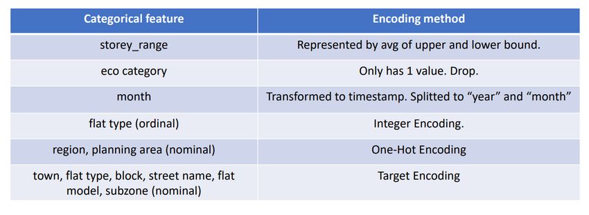
Fig. 4. Encoding of Categorical Features

                                                                   value, so we drop that column. What’s more, ’month’ feature
                                                                   has format of ”Year-Month”, which contains the temporal
                                                                   informaition. Instead of simply treating them as sets of values.
                                                                   We transformed it into timestamps, and also splitted it into two
                                                                   two features ”year” and ”month” to capture richer information.
                 Fig. 1. Basic information of dataset
                                                                      One way of encoding is called integer encoding, which is
                                                                   simply using integers to represent different values of variables.
                                                                   Since the integers have natural internal ordering, this method
                                                                   can only be applied on ordinal variables, where the variables
                                                                   also have natural internal ordering. We observed that, feature
                                                                   ”flat type” has an internal ordering in the size of the house.
                                                                   There are seven different values, ’1 room’ ’2 room’ ’3 room’
         Fig. 2. flat model                 Fig. 3. flat type      ’4 room’ ’5 room’ ’executive’ and ’multi generation’, which
                                                                   are encoded as 1-7.
                                                                      Another common way of encoding is One-Hot, which means
B. Feature Engineering                                             to expand the variable to a dimension of number of unique
                                                                   values, and label the true unit as ”1”, while others remain
   Feature engineering is a process of transforming the given
                                                                   zero. This method can be applied on nominal variables where
data into form of which is easier to explain and interpret. Here
                                                                   there’s no natural orders. However, one-hot encoding is not
we aim at making the features better suited to our problem
                                                                   suitable for features with too many values, or it will add large,
at hand, the prediction of HDB resale price. Some features
                                                                   sparse dimensionality of spaces and heavy burden. We finally
need to be encoded or transformed, some new features need
                                                                   applied One-Hot encoding on feature ”region” and ”planning
to be invented. In this section, we focus on transformation and
                                                                   area”.
encoding of existing features.
                                                                      For those nominal variables with large number of unique
   For a feature to be useful, it must have a mathematical
                                                                   values, Target Encoding becomes the best choice. Target
relationship to the target for models to learn. For numeric
                                                                   encoding is basically replacing a categorical value with the
features, we decided to leave them as they are, since after
                                                                   mean of the target variable (resale price). We used target
several experiments, we found that both clustering technique
                                                                   encoding to encode features ’town’, ’flat type’, ’block’, ’street
and normalization do not contribute to our final result. The
                                                                   name’, ’flat model’ and ’subzone’. Therefore, target encoding
feature ”elevation” contains only 1 value ”0.”, which is con-
                                                                   turns out to be the most popular and applicable way in our
sidered equivalent to all data points. So we simply drop this
                                                                   case.
column.
   However, there’re still many features that are given in non-    C. Feature Generation
numeric form, which are categorial features. These features           In addition to the features that the core dataset file contains,
can take on values from a limited set of values. Some algo-        we came up with some new features that can improve the
rithms like decision tree can directly learn from categorical      accuracy of our predictions.
data, but many machine learning techniques and algorithms             There are two features related to time in the original data:
cannot operate on label data directly. They require all input      ”month” and ”lease commence date”. The feature ”month”
variables to be numeric. That’s why for each category, we need     does not only include the information about which month
to introduce an integer number representing it.                    but also which year when a HDB flat was sold. And the
   First of all, we found that categorial feature ’storey range’   feature ”lease commence date” tells us when the lease for
is actually a clustering of numeric feature ’storey’, saved in     a flat commenced.
object data type. Therefore, we using the average of upper               a) Year of the sale: We can know the year when the sale
and lower bound to represent this feature, which somehow           happened from the existing feature ”month”. This feature can
reflects the difference of storey height among HDB flats. After    be helpful because the price of a flat may be influenced by
that, we observed that feature ’eco category’ contains only 1      the economy and policies of the year.
• year: This feature represents the year when the sale we generate new features to represent the number of facilities
happened. within a radius of 2 kilometers:
b) Number of years before sale: By subtracting the • num of cc: The number of commercial centres within a
feature ”year” and the feature ”lease commence date”, the radius of 2 kilometers to a HDB flat.
new feature named ”year before sale” is obtained. This new • num of gov market: The number of markets within a
feature can be used to measure how old and new a HDB radius of 2 kilometers to a HDB flat.
is, which buyers will pay attention to in real resale market. • num of pri school: The number of primary school
Compared to an old flat that could have many inevitable within a radius of 2 kilometers to a HDB flat.
problems like conduit ageing, a relatively new flat is usually • num of sec school: The number of secondary school
preferred by buyers. within a radius of 2 kilometers to a HDB flat.
• num of shopping mall: The number of shopping malls
• year before sale: This feature represents the number of
years between the time when the lease for a flat com- within a radius of 2 kilometers to a HDB flat.
• num of train station: The number of train stations within
menced and the time when this sale happened.
a radius of 2 kilometers to a HDB flat.
D. Auxiliary Data Using c) Demand for Sold Flats: We collected ”resale price
a) Distance to nearest facilities: Although the corre- index” and ”demand for sold flats” as additional data from
lation coefficients between both ‘latitude’ and ‘longitude’ Data.gov.sg. However, since the ”resale price index” can be
and ‘resale price’ are very low, we decide to use these two considered our target in a sense, we dropped it and only took
features to relate an HDB flat’s location to its surrounding ”demand for sold flats” as additional data feature. ”Demand
facilities(leveraging the auxiliary data). It is because that the for sold flats” does not perform well and was not used in our
value of a flat is not only depend on its own attributes, but final experiment.
also on how easy and convenient its neighborhood is to live E. Feature Selection
in. For example, buyers who have children are likely to buy
Combining correlation analysis and the importance weight
a flat that near to schools; buyers who enjoy going shopping
of features, we select features that have both a relatively
may want to live near shopping malls.
high correlation and importance weight to train the model.
To assess the degree of the convenience of a flat, we
For features in original data, we decided to drop block, town
firstly calculated the distance between flats and every facilities
and street name. For features calculated from auxiliary data,
(including MRT stations, shopping malls, commercial centers,
features selected are as follows.
markets, and schools), by using features ‘latitude’ and ‘longi-
• num of cc
tude’.
• num of gov market
Then, we take the smallest distance to certain type of facility
• num of pri school
as a new feature, which represents how far the nearest facility
• num of sec school
is from the HDB flat. The new features we generated are as
• num of shopping mall
follows:
• num of train station
• to commercial: The distance between a HDB flat and the
It is worth noting that, even if we thought feature correlation
nearest commercial centre.
to target as an important criterion to select feature, the corre-
• to gov markets: The distance between a HDB flat and
lation value does not always matching the feature importance
the nearest market.
when trained on regressors. Here are two histgrams, showing
• to malls: The distance between a HDB flat and the
the correlations and importance of the 5 most important
nearest shopping mall.
features when applied on XGBoost:
• to primary schools: The distance between a HDB flat
and the nearest primary school.
• to secondary schools: The distance between a HDB flat
and the nearest secondary school.
• to train stations The distance between a HDB flat and
the nearest train station.
Fig. 5. correlations Fig. 6. importance to XGBoost
It is noteworthy that, when computing the distance to
train(MRT) station, we took the ”opening year” into consider- We can see from these two histgrams , feature ”centre
ation, which means that only stations opening before the sale region” is fairly important to XGBoost when doing regression,
year are considered. Besides, not all of these new features are but the correlation of it is not the highest.
finally used in our experiment. According to the experiment
results, some of them are helpful, but others are not. IV. DATA M INING M ETHODS
b) Number of facilities in the neighborhood: Besides the The resale price of HDB flats is continuous variable, there-
distance to the nearest facilities, we also assume the number of fore, we need regression model to predict on it. Different kinds
facilities in the neighborhood an important factor. Therefore, of regressors are trained on the data and evaluated.A. Models V. E VALUATION AND I NTERPRETATION
1) Linear Regression: The first model we try is basic Linear Regression gets the worst score. The cross-validation
linear regression. However, the result is not good because the score with default parameters is around 50000. Because linear
model is rather biased, the output is always a regression line, regression is biased, the output is always a regression line,
plane or hyperplane, so it might be restrictive for this dataset. plane or hyperplane, so it might be restrictive for this dataset.
Therefore, linear regression is taken out of consideration. Random forest get the highest score with default parameters,
Seeing the poor performance of linear regression, we seek for which is over 17000. The superior performance of random
more complicated models for the prediction. forest mainly depends on randomly sampled samples and
2) Random Forest: Random forest is the second model we features and integrated algorithms. The former makes it more
try. It has a much better performance than linear regression. stable against overfitting, and the latter makes it more accurate.
This is the model that we got a relatively high score for the first Xgboost is the second best with default parameters. The
time. However, long training time makes further improvement difference between Xgboost and random forest is small, xg-
based on random forest difficult. When we want to test the boost gets over 19000. However, with hyper-parameter tuning,
effect of feature engineering, or try hyper-parameter tuning, Xgboost got the highest score. Xgboost performs well because
we found it takes too much time to train the random forest it improves accuracy by continuously improving the loss
regressor, because trees in the forest are trained sequentially. residual and reinforces the knowledge learned by mistakes.
In this situation, further improvement done with random forest Final Result: We finally got 15698.7 on Kaggle competition,
is not practical and efficient for us. ranking 15th.
3) Xgboost: In boosting methods, trees can be trained
in parallel. Besides, training xgboost can be speed up by
with GPU. Therefore, we switched to Xgboost seeking for
better performance as well as shorter training time. After
first trying Xgboost with default parameters, we get a score
around 19000, which is not bad. For the training time, it takes
around 20 minutes on CPU with default parameters. And after
Fig. 7. Encoding of Categorical Features
setting the training on GPU, it only takes around 2 minutes.
Therefore, Xgboost is chosen as our final prediction model.
After finalizing our choice, we also did hyper-parameter tuning B REAKDOWN OF W ORKLOAD
based on Xgboost to make further improvements. Here is a breakdown of our workload.
B. Hyper-parameter Tuning
TABLE I
Xgboost is a tree-based model, therefore, adjusting parame-
ters for tree booster must have an influence on the performance Team Members
Tasks Xiong Kexin Yao Yihang Liu Xing
of the tree. For tree booster parameters, we first use grid search
Exploratory Data Analysis ! ! !
to find the best parameter for max depth and n estimators. Preprocessing ! ! !
After grid search, we find the best max depth is around 12, Model Training ! ! !
and the best n estimators is around 500. If the max depth Report Writing ! ! !
and the number of estimators is greater, the scores goes
down because of overfitting. Next, learning rate and mini-
mum child weight is found with max depth and n estimators
fixed. Minimum child weight is another parameter for tree
booster, it is the minimum sum of instance weight (hessian)
needed in a child. If the tree partition step results in a leaf node
with the sum of instance weight less than min child weight,
then the building process will give up further partitioning.
Min child weight is a parameter relevant to the number of
the features. We need to adjust it manually every time when
the number of features is changed, but the best values are from
10 to 16. Learning rate is step size shrinkage used in update to
prevents overfitting. After each boosting step, we can directly
get the weights of new features, and eta shrinks the feature
weights to make the boosting process more conservative.
Because of the synergy between multiple parameters, learning
rate is first adjusted through grid search and then adjusted in
a small range manually and the best learning rate is around
0.06.You can also read