Private Continual Release of Real-Valued Data Streams - Date: February 26, 2019 Victor Perrier, Hassan Jameel Asghar, Dali Kaafar Macquarie ...
←
→
Page content transcription
If your browser does not render page correctly, please read the page content below
Private Continual Release of
 Real-Valued Data Streams
                   Date: February 26, 2019
                        Victor Perrier,
                    Hassan Jameel Asghar,
                           Dali Kaafar
     Macquarie University, Data61 (CSIRO), ISAE-SUPAERO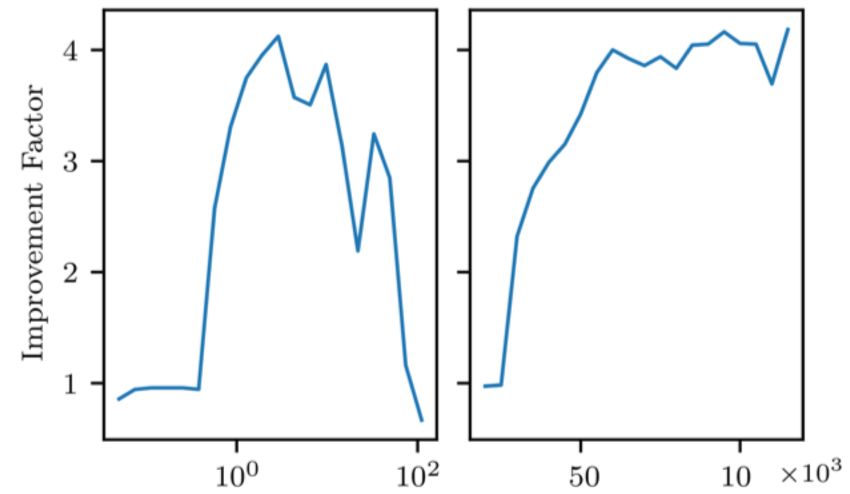
Streaming Data and Statistics
• Real-time monitoring of customer data can improve services
   • Real-time updates
   • Analysts/planners can optimize services

          Service     Event                 Real-time statistics
          Energy      Smart-meter reading   Electricity usage in a neighborhood
          Transport   Tap-on/off time       Peak hour commute times
          Retail      Supermarket bill      Average expenditure in a supermarket
          Location    Check-in/out time     Average time spent in a restaurant

                                                                                   2
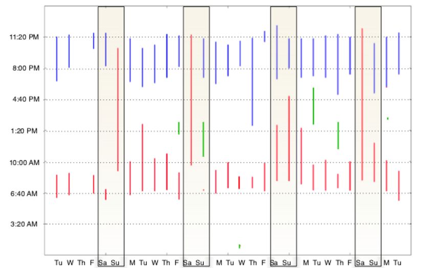
Issue: Privacy                       Smart meter readings

• Raw stats may reveal
  sensitive events
   • Unusual presence at home
     (smart meter)
   • Trip to beach instead of work
     (transport)

• Events (observations) can be
  linked to real-life activities
  [MSF+10]
                                        Unusual activity [MSF+10]

                                                                    3
✏
                                                                           on a given day. Notice that this is significantly less than
            Since GS = B , we get a linear term in B . We will             the total time possible in a 24 hour period, which is
            use this algorithm as the building block, but we shall         obviously 1,440 minutes.

Privacy-Preserving Statistics
            find ways to improve the dependence on B . Our gain
            will be through the assumption that actual distribution
            of the string      is concentrated far below B . We will                          CDF of observations
            later justify this assumption by analyzing two real-world
            datasets. Then, instead of using the global sensitivity,
• Differential privacy a natural candidate
            we shall use smooth sensitivity tailored to a threshold
               ⌧ B , and therefore we expect considerable gain in
   •   Most⌧utility.
              work     on static databases

                                                                             % readings
   • Some work on binary data streams [DNPR10,
     CSS11]
         A. Motivation
               We consider scenarios where the upper bound B on a
            generic element of the incoming stream is overly conser-
• Our problem
            vative resulting in utility that is begging to be improved
            in practice. Consider the following likely scenarios
   •   Data from
               • Thean    event
                      bound        is real-valued
                              B might                      withinFor
                                         not be known in advance.    a                                                    !
       public upper        a bound!
                         bound
                 instance,           on the expenditure during a trip to                                               public
                                                                           Fig. 2: Histogram of journey times on Sydneybound
                                                                                                                        trains on
                 the supermarket. Any guess on the bound B would
   •   Release updated
                 be taking intosum/average
                                 account instances atofeach   event
                                                        unusually  high
                                                                           a particular day What is the scale of the x-axis.

   •   Event-level     privacy
                 spendings.   This will result in a very conservative
                                                                              Likewise, we see a similar trend in the total expen-
                 upper bound.
        • Peculiar   events protected
               • In some cases, a natural bound B exists. For in-
                                                                           diture during a trip to a supermarket chain in Australia
                                                                                                                        time
                                                                           on a given day. Converted into an empirical cumulative
                 stance, the commute time per day has a natural
                                                                           distribution function (CDF), the two distributions
                                                                                      events                            4       are
                 bound of B = 24 hours. However, most commute
                                                                           shown in Figures 3 and 4 respectively. An interesting
for strings of length n, where                              trains on a particular day (including multiple trips). We
                                     ✓       r                ◆                can see that the peak is around 20 to 30 mins, and very
                                           1      1
                             ↵ = O GS ·       8 ln log2 (n)1.5 .               few customers take more than 150 minutes of train ride
                                           ✏
                                                                               on a given day. Notice that this is significantly less than
How to Release the Average?
              Since GS = B , we get a linear term in B . We will
              use this algorithm as the building block, but we shall
                                                                               the total time possible in a 24 hour period, which i
                                                                               obviously 1,440 minutes.
              find ways to improve the dependence on B . Our gain
              will be through the assumption that actual distribution
                                                                                                    CDF of observations
•   Basic: addofLaplace
                  the string noise      of scalefar!below
                                  is concentrated      to each
                                                            B . We will
    observation
              later justify this assumption by analyzing two real-world
              datasets.
     • Error !"    afterThen,    instead of using the global sensitivity,
                          " events
              we shall use smooth sensitivity tailored to a threshold
              ⌧ ⌧ B , and therefore we expect considerable gain in
•   Generalized
              utility.binary stream algorithm fairs better

                                                                                  % readings
      • Error !log & " [DNPR10, CSS11]
                   A. Motivation
             We consider scenarios where the upper bound B on a
• Problem: generic
           error     still proportional to !
                   element of the incoming stream is overly conser-
      • In manyvative resulting !
                 situations     in is toothat
                                   utility loose    or unknown
                                              is begging to be improved
            • E.g.,inUnlikely
                      practice.someone    commuting
                                Consider the following for  fullscenarios
                                                        likely   24 hours!
                                                                                                         '                         !
                     •  The bound B might not be known in advance. For                               threshold
      •   Most readings        concentrated
                        instance,  a bound on thebelow        during a trip to'
                                                          a threshold
                                                  expenditure                                                                   public
                                                                                Fig. 2: Histogram of journey times on Sydney bound
                                                                                                                                trains on
                        the supermarket. Any guess on the bound B would
                                                                                a particular day What is the scale of the x-axis.
      •                 be  taking  into account
          If ' known, error is only 'log & "     instances of unusually  high
                        spendings.
             • Significant           This will result in a very conservative
                            if !: ' large                                          Likewise, we see a similar trend in the total expen
                        upper bound.
                                                                                diture during a trip to a supermarket chain5 in Australia
                      • In some cases, a natural bound B exists. For in-
Validation of Data Concentration
                                                                              Train trips
• Is data really concentrated well below a
  conceivable !?

                                                            % trips
• Train trips dataset
   • 50 million trips over four weeks (Sydney, Australia)                        minutes
   • Conceivable bound ! = 24 hours
                                                                             Supermarket

• Supermarket dataset

                                                            % transactions
   • 140,000 transactions by 1,000 customers (Australia)
   • Conceivable bound ! = ?

                                                                                  dollars
                                                                                            6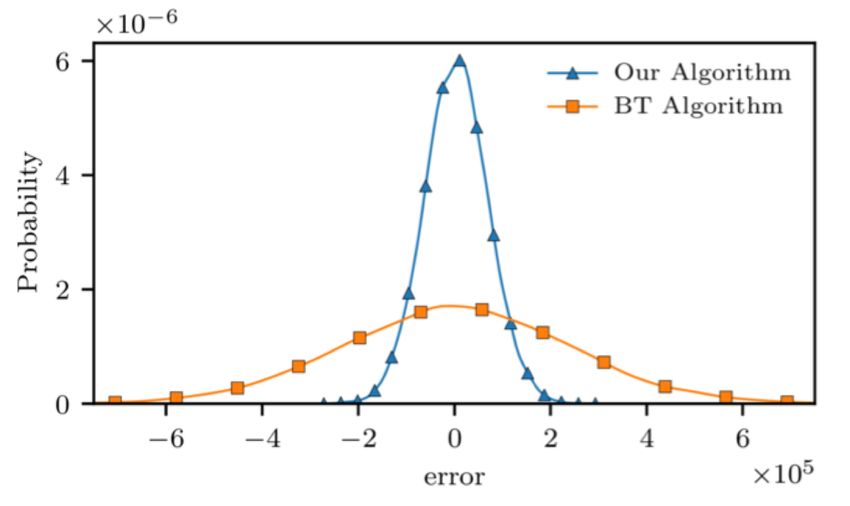
How to Estimate Threshold with Privacy?
• Need to observe a subset ! of observations
  – time lag                                                                Stream Readings
                                                   90
                                                   80

• Time lag needs to be optimized for accuracy      70

                                                   60
   • Too early: high outlier error                 50

   • Too late: marginal gain (may just use " as    40
                                                   30
     estimate)                                     20

                                                   10
                                                   0
                                                        1   2   3   4   5     6   7   8   9   10   11   12   13   14   15

• Naively estimating # violates privacy                                    !
                                                                        Time lag
                                                                                                                       $

   • E.g., maximum of ! observations is an exact
     event!

                                                                                                             7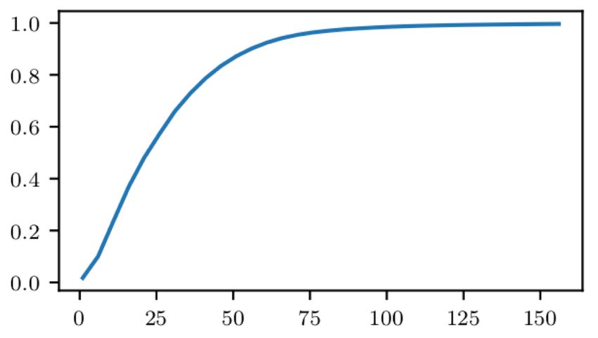
Our Work
• A method to estimate threshold ! using a subset of observations
   • With differential privacy
   • and utility optimized for moving average

• Mechanism is generic – can also be used for
   • Average over a sliding window
   • Releasing histogram of streaming data
   • Estimating scale of distribution

                                                                    8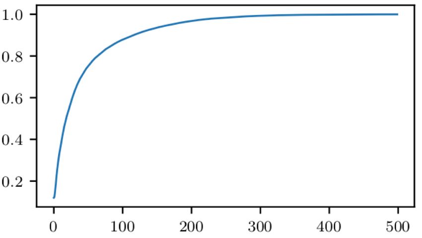
Background: Binary Tree Algorithm

• Binary tree (BT) algorithm [DNPR10, CSS11]
  • Find at most log $% nodes in tree whose union
    equals sum up to & events
                                 '()*+ ,                ',
  • Add Laplace noise of scale      -
                                           instead of    -

• Goal: Use BT as sub-module but noise
  scaled to . instead of /
                                                             Computing private sum of first 7 observations

                                                                                                   9
Global Mechanism
1. Estimate threshold ! using first " observations using budget #$

                                    %
2. Use Laplace noise with scale to release sum of first "
                               &'
   observations

3. Update & release sum for each event after " with Laplace noise of
   scale ! log + ,/# using BT algorithm

• Overall: (#, 0)-differential privacy

                                                                       10
What are the Choices for Threshold?
• False starts
• Differentially private max of ! values?
• max function is highly sensitive
• Adjacent streams can differ by any value in [0, %] Distribution of '
• Standard deviation of distribution of '?
• Need to know distribution in advance
( fraction of values
• Statistic of choice: (-quantile
• E.g., ( = 0.005 (0.5% of values)
,(
(-quantile
11Privately Estimating !-Quantile
• Need to estimate !-quantile through first " readings
• Satisfying # ≫ " ≫ 1/! required for stable estimate of !
• Roadmap
• Obtain the empirical estimate (' ! of (!
• Add differentially private noise to (' !
• Set the result as threshold )
• Complication: cannot use Global Sensitivity (GS) for DP noise
• Maximum change in function over all adjacent streams
• GS of !-quantile is close to *
12Using Smooth Sensitivity
• Local sensitivity (LS)
• Maximum change in !-quantile over streams adjacent to input stream only
• Unfortunately, LS itself can be sensitive
• E.g., big differences in LS over nearby streams
• Smooth sensitivity (SS) [NRS07]
• " #, # % : Hamming distance between streams # and # %
234 .,. /
• SS(#, () = max./ {1 5 LS./ }
• Smooths out change in LS as we move away from input stream
13Privately Obtaining the Threshold
• Obtain threshold as
! = $# %+ Laplace noise with SS
• We have swept some details under the
rug
• $# % and ! should be ≥ $% to bound error
• We assume $# % ≥ $%
14Utility Analysis
• Light-tailed distributions Train trips dataset
• Lighter than exponential distribution with the
same !-quantile
• True for train trips and supermarket datasets
for sufficiently small !
• If distribution is light-tailed
• We show that error "log & '/) (as required)
• Note: Privacy definition not dependent on
distribution assumption ! = 0.005-quantile
15Utility Analysis for Light-tailed Distributions
• Exponential distribution has the property
!" # $ ≥ !&' for all $ ≥ 1
• For light-tailed distributions: !) " # $ ≥ !&'
• Idea:
• Estimate "-quantile using 1/" readings
!" !& '
• Set threshold + to !) " # $
• Benefits: ≈ + = !) " # $
• Estimate threshold with a much smaller time lag ,
• Minimise outlier error project
. estimate
• - log 3 4
/
16What Values to Use in Practice?
• Improvement Factor (IF) metric
• Ratio of error through BT versus Impact of epsilon Impact of time lag
our method
• Epsilon: IF increases with larger !
but then drops
• Due to truncation: any value greater
than threshold is fixed to threshold
• Time lag: Noticeable increase in
impact factor with " ≈ 50,000
! "
17Heuristics for Choosing Parameters
• Optimization suggests
Parameter Interpretation Value
! !-quantile 0.005
" Shifting !-quantile Between 1 and 2
#$ Budget to estimate threshold 0.8 of overall privacy budget
#% Budget to release sum of first & terms Derive from #$
& Time lag 50,000
18Experimental Evaluation
Train trips dataset
• Max error on the sum (at step !)
• 20k repetitions
• Train trips
• ! = 250, 000, 000
• " = 50,000
• # = 1440 mins (24 hrs)
• Improvement factor: 3.5
Supermarket dataset
• Supermarkets
• ! = 150, 000
• " = 50,000
• # = 3,000 dollars
• Improvement factor: 9
19Discussion
• Improved private release of moving average if distributions are light-tailed
• Question: which data have light-tailed distribution?
• Any data coming from short-lived, time constrained events
• Smart-meter data
• Phone-call durations
• Length of posts (on social media)
• Daily average inter-arrivals of check-in times
• Heavy-tailed distributions are not “directly” time-constrained
• Income distribution
• File sizes in computer systems
20Conclusion
• Shown a way to privately estimate the bulk of a distribution of streaming real-
valued data
• Can be estimated by sacrificing a time lag
• Heuristics for choosing parameters in practice
• In worst-case, threshold is close to public bound !
• We do not need to abort as in the propose-test-release approach [DL09]
• Moving average release is just one application – can be used in other applications
21Questions
22References
• [CSS11]Chan, T.H.H., Shi, E. and Song, D., 2011. Private and continual release of
statistics.ACM Transactions on Information and System Security (TISSEC), 14(3), p.26.
• [DL09] Dwork, C. and Lei, J., 2009, May. Differential privacy and robust statistics.
In STOC (Vol. 9, pp. 371-380).
• [DNPR10] Dwork, C., Naor, M., Pitassi, T. and Rothblum, G.N., 2010, June. Differential
privacy under continual observation. In Proceedings of the forty-second ACM symposium
on Theory of computing (pp. 715-724). ACM.
• [MSF+10] Molina-Markham, A., Shenoy, P., Fu, K., Cecchet, E. and Irwin, D., 2010,
November. Private memoirs of a smart meter. In Proceedings of the 2nd ACM workshop
on embedded sensing systems for energy-efficiency in building (pp. 61-66). ACM.
• [NRS07] Nissim, K., Raskhodnikova, S. and Smith, A., 2007, June. Smooth sensitivity and
sampling in private data analysis. In Proceedings of the thirty-ninth annual ACM symposium on
Theory of computing (pp. 75-84). ACM.
23You can also read