Radar Wind Profiler (RWP) and Radio Acoustic Sounding System (RASS) Instrument Handbook - DOE/SC-ARM-TR-044
←
→
Page content transcription
If your browser does not render page correctly, please read the page content below
DOE/SC-ARM-TR-044

Radar Wind Profiler (RWP) and Radio Acoustic
Sounding System (RASS) Instrument Handbook

P Muradyan R Coulter

March 2020
DISCLAIMER

This report was prepared as an account of work sponsored by the U.S.
Government. Neither the United States nor any agency thereof, nor any of
their employees, makes any warranty, express or implied, or assumes any
legal liability or responsibility for the accuracy, completeness, or
usefulness of any information, apparatus, product, or process disclosed, or
represents that its use would not infringe privately owned rights. Reference
herein to any specific commercial product, process, or service by trade
name, trademark, manufacturer, or otherwise, does not necessarily
constitute or imply its endorsement, recommendation, or favoring by the
U.S. Government or any agency thereof. The views and opinions of
authors expressed herein do not necessarily state or reflect those of the
U.S. Government or any agency thereof.
DOE/SC-ARM-TR-044

Radar Wind Profiler (RWP) and Radio
Acoustic Sounding System (RASS)
Instrument Handbook

P Muradyan
R Coulter
Both at Argonne National Laboratory

March 2020

Work supported by the U.S. Department of Energy,
Office of Science, Office of Biological and Environmental Research
P Muradyan and R Coulter, March 2020, DOE/SC-ARM-TR-044

 Acronyms and Abbreviations
ACAPEX ARM Cloud Aerosol Precipitation Experiment
AMF ARM mobile facility
ARM Atmospheric Radiation Measurement
AT Acceptance Test
BBSS balloon-borne sounding system
BSRWP beam-steered radar wind profiler
CF Central Facility
COMBLE Cold-Air Outbreaks in the Marine Boundary Layer Experiment
DQO Data Quality Office
ENA Eastern North Atlantic
FA final amplifier
FFT fast Fourier transform
FMC-BL full motion control−boundary layer
GPS Global Positioning System
IMU Inertial Measurement Unit
MAGIC Marine ARM GPCI Investigations of Clouds
MARCUS Measurements of Aerosols, Radiation, and Clouds over the Southern Ocean
MII Modulator, Intermediate Frequency and Interface
MOSAIC Multidisciplinary Drifting Observatory for the Study of Arctic Climate
NSA North Slope of Alaska
QC quality control
RASS radio acoustic sounding system
RWP radar wind profiler
SGP Southern Great Plains
SNR signal-to-noise ratio
UTC Coordinated Universal Time
VAP value-added product

 iv
P Muradyan and R Coulter, March 2020, DOE/SC-ARM-TR-044

 Contents
Acronyms and Abbreviations ...................................................................................................................... iv
1.0 General Overview ................................................................................................................................. 1
2.0 Contacts ................................................................................................................................................ 1
 2.1 Mentors ........................................................................................................................................ 1
 2.2 Vendor/Instrument Developer ...................................................................................................... 2
3.0 Deployment Locations and History ...................................................................................................... 2
4.0 Near-Real-Time Data Plots .................................................................................................................. 3
5.0 Data Description and Examples ........................................................................................................... 3
 5.1 Data Formats ................................................................................................................................ 3
 5.1.1 Wind Profile Data.............................................................................................................. 3
 5.1.2 Virtual Temperature Profile Data ...................................................................................... 5
 5.1.3 Precipitation Operation ..................................................................................................... 7
 5.2 Data File Contents ........................................................................................................................ 8
 5.2.1 Data Types......................................................................................................................... 8
 5.2.2 Primary Variables and Expected Uncertainty ................................................................... 9
 5.2.3 Data Quality Flags........................................................................................................... 10
 5.3 Annotated Examples. ................................................................................................................. 12
 5.4 User Notes and Known Problems .............................................................................................. 12
 5.5 Frequently Asked Questions ...................................................................................................... 12
6.0 Data Qualiy ......................................................................................................................................... 14
 6.1 Data Quality Health and Status .................................................................................................. 14
 6.2 Data Reviews by Instrument Mentor.......................................................................................... 14
 6.3 Data Assessments by Site Scientist/Data Quality Office ........................................................... 15
 6.4 Value-Added Products ............................................................................................................... 15
7.0 Instrument Details............................................................................................................................... 16
 7.1 Detailed Description................................................................................................................... 16
 7.1.1 List of Components ......................................................................................................... 16
 7.1.2 System Configuration and Measurement Methods ......................................................... 16
 7.1.3 Specifications .................................................................................................................. 18
 7.2 Operation and Maintenance ....................................................................................................... 18
 7.2.1 User Manual .................................................................................................................... 18
 7.2.2 Routine and Corrective Maintenance Documentation .................................................... 18
 7.2.3 Software Documentation ................................................................................................. 18
 7.3 Glossary...................................................................................................................................... 18
 7.4 Acronyms ................................................................................................................................... 18
8.0 Citable References .............................................................................................................................. 19
9.0 Bibliography ....................................................................................................................................... 20

 v
P Muradyan and R Coulter, March 2020, DOE/SC-ARM-TR-044

 Figures
1 Calculated moments for the vertical beam (precpmom, high power mode) at SGP I9, Billings,
 Oklahoma on 2018-04-21. ...................................................................................................................... 5
2 RWP low- (left) and high- (right) power consensus-averaged winds recorded on 2020-02-26 at
 the SGP I8 Facility. ................................................................................................................................ 5
3 An example of a 24-hour display of RASS virtual temperature (units in Co). ....................................... 6
4 An example of adaptive algorithm’s operation switching from wind mode to precipitation mode
 only when precipitating conditions have been identified. ...................................................................... 7
5 Precipitation effect on the consensus winds. ........................................................................................ 10
6 Low- (bottom) and high- (top) power winds (left) and SNR (right) affected by migrating birds. ....... 11

 Tables
1 ARM RWP deployment history at observatories and mobile facilities.................................................. 2

 vi
P Muradyan and R Coulter, March 2020, DOE/SC-ARM-TR-044

1.0 General Overview
 The radar wind profiler (RWP) is an active remote-sensing instrument that can routinely, and virtually
 unattended, observe wind and turbulence in the troposphere through scattering from clear-air irregularities
 of the atmospheric refractive index (Gage and Balsley 1978). The principle of Doppler radars in general is
 based on sending electromagnetic pulses in the vertical and several tilted directions (vertical and oblique
 beams) and measuring the signal that is scattered back by atmospheric turbulence at all heights and
 received at the antenna. The RWPs provides measurements of backscattered signal strength and wind
 profiles nominally between 0.1 km and 6 km. The RWP operation assumes that the wind field is
 homogeneous over the spatial separation of the antenna beams, which is a safe assumption under stable
 atmospheric conditions. However, the wind may be different between the beams due to significant
 changes in the wind field, resulting in erroneous wind calculations. Therefore, the radial measurements
 are averaged over a sufficient time period to validate the assumption of homogeneity.

 Prior to 2010, a radio acoustic sounding system (RASS) was incorporated with the RWP to obtain virtual
 temperature profiles at the Atmospheric Radiation Measurement (ARM) user facility’s Southern Great
 Plains (SGP) observatory. However, after 2011 the acoustic transmitters are no longer included in the
 systems. 915 MHz RWPs are deployed at ARM sites in the United States, while for most foreign
 deployments 1290 MHz systems are used.

 The second ARM Mobile Facility (AMF2) was designed to be frequently deployed at sea; therefore, it has
 a 1290 MHz full motion control−boundary layer (FMC-BL) RWP system developed by DeTect, Inc.
 (currently Radiometrics) that is capable of changing the beam-pointing angle on a pulse-by-pulse basis so
 that it can compensate for ship motions during shipborne deployments.

2.0 Contacts

 2.1 Mentors
 Paytsar Muradyan
 Environmental Science Division
 Argonne National Laboratory
 Phone: (630) 252-1657
 Email: pmuradyan@anl.gov

 Richard Coulter
 Environmental Science Division
 Argonne National Laboratory
 Phone: (630) 252-5833
 Email: rlcoulter@anl.gov

 1
P Muradyan and R Coulter, March 2020, DOE/SC-ARM-TR-044

 2.2 Vendor/Instrument Developer
 Vaisala Corporation
 194 South Taylor Avenue
 Louisville, Colorado 80307
 Phone: (30)3-499-1701
 Fax: 303-499-1767

 Scintec Corporation
 1730 38th Street
 Boulder, Colorado 80301
 Phone: (30)3-666-7000
 Fax: (303)-666-8803

 Radiometrics
 4909 Nautilius Court North, Suite 110
 Boulder, Colorado 80301
 Phone: (303)-449-9192
 Fax: 303)-786-9343

 3.0 Deployment Locations and History
 Table 1 shows RWP deployment history at ARM observatories and mobile facilities. Locations marked
 with (*) are shipborne mobile deployments, and the field campaign name is used as its location.

 Table 1. ARM RWP deployment history at observatories and mobile facilities.
 Site Location Facility Mfr Freq Description/ Start date End date
 ID (MHz) Modes (MM/YYYY) (MM/YYYY)
 C1 Vaisala 915 Winds/RASS 11/1992 03/2011
 C1 Vaisala 915 Winds/Precip 03/2011 03/2019
 Lamont, OK
 C1 Vaisala 915 Adaptive 03/2019 08/2019
 C1 Radiometrics 915 Winds/Precip 08/2019 Present
 Beaumont, KS IF1 Vaisala 915 Winds 09/1996 03/2011
 Medicine Lodge, KS IF2 Vaisala 915 Winds 09/1996 09/ 2008
SGP Meeker, OK IF3 Vaisala 915 Winds 09/1996 02/2009
 IF8 Vaisala 915 Winds/Precip 05/2011 05/2018
 Tonkawa, OK
 IF8 Vaisala 915 Adaptive 05/2018 Present
 IF9 Vaisala 915 Winds/Precip 05/2011 03/2019
 Billings, OK
 IF9 Vaisala 915 Adaptive 03/2019 Present
 IF10 Vaisala 915 Winds/Precip 04/2011 03/2019
 Lamont, OK
 IF10 Vaisala 915 Adaptive 03/2019 Present
NSA Barrow, AK C1 Vaisala 915 Winds/Precip 04/2001 10/2017
ENA Graciosa, Azores C1 Scintec 1290 Winds/Precip 09/2014 Present
AMF1 Niamey, Niger NIM M1 Vaisala 915 - 04/2006 01/2007
 Black Forest, Germany FKB M1 Vaisala 1290 - 03/2007 08/2007

 2
P Muradyan and R Coulter, March 2020, DOE/SC-ARM-TR-044

 Shouxian, China HFE M1 Vaisala 1290 - 09/2008 12/2008
 Azores GRW M1 Vaisala 1290 - 04/2009 12/2010
 Nainital, India PGH M1 Vaisala 1290 - 11/2011 03/2012
 Cape Cod, MA PVC M1 Vaisala 915 - 07/2012 07/2013
 Manacapuru, Brazil MAO M1 Vaisala 1290 - 03/2014 12/2015
 Ascension Island ASI M1 Vaisala 1290 - 06/2016 10/2017
 Walla Walla, WA WWL Vaisala 915 - 05/2015 05/2017
 Cordoba, Argentina COR M1 Vaisala 1290 - 09/2018 05/2019
 Nordmela, Norway ANX M1 Vaisala 1290 - 09/2019 -
AMF2 Steamboat Springs, CO SBS M1 Vaisala 915 - 11/2010 03/2011
 Gan Island, Maldives GAN M1 Radiometrics 1290 - 11/2011 02/2012
 MAGIC* MAG M1 Radiometrics 1290 - 12/2012 06/2013
 Hyytiala, Finland TMP M1 Radiometrics 1290 - 01/2014 08/2014
 ACAPEX* ACX M1 Radiometrics 1290 - 01/2015 02/2015
 McMurdo, Antarctica AWR M1 Radiometrics 1290 - 12/2015 01/2017
 MARCUS* MAR M1 Radiometrics 1290 - 10/2018 03/2018
 MOSAIC* MOS M1 Radiometrics 1290 - 09/2019 -
AMF3 Oliktok, AK M1 Scintec 915 Winds/Precip 08/2014 08/2017

 4.0 Near-Real-Time Data Plots
 Data collected by the RWPs can be viewed in near-real time through the Data Quality Office’s (DQO)
 Quick Plot Browser.

 5.0 Data Description and Examples

 5.1 Data Formats

 5.1.1 Wind Profile Data

 The data produced by this instrument come in three forms: raw spectra, moments, and time-averaged
 profiles.

 • Spectra: The spectra are the most basic form of data produced by the present version of this
 instrument. The method by which the spectra are obtained is discussed below in section 7.1.2. They
 display the energy content of the scattered signal over the range of Doppler shifts observed from each
 pointing direction and power level of the wind profiler. There is a single spectrum for each range
 gate, pointing direction, and power level, and each spectrum represents an average of several
 (e.g., 60) individual spectra obtained over several seconds (e.g., 30).
 • Moments: The moments data are calculated directly from the spectral data by integrating across the
 Doppler frequency domain, and basically represent the spectrum as a whole. At each range gate,
 beam pointing direction, and power level, four quantities are calculated:

 3
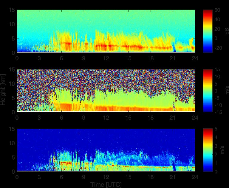
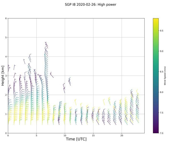
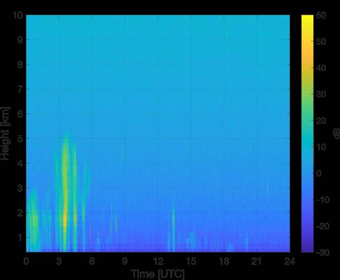
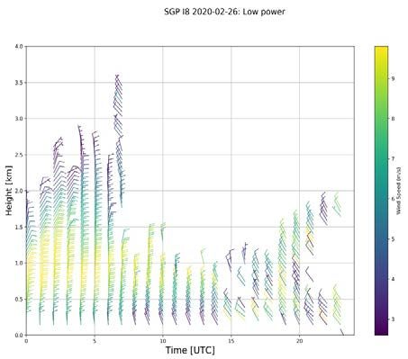
P Muradyan and R Coulter, March 2020, DOE/SC-ARM-TR-044

 1. Mean Doppler shift: The first moment of the spectrum, fD calculated roughly as:

 2 2

 = � ( )� � ( )
 = 1 = 1
 Eq. 1

 where S(f) is the power at frequency f and f1 and f2 are the minimum and maximum
 frequencies, chosen about a mid-point frequency associated with the maximum signal
 power level.

 2. Doppler width: The width of the spectrum, VD, calculated as:

 2 2

 = 2� �(( − )2 ( ))� � ( ) Eq. 2
 = 1 = 1

 3. Noise level: This value is calculated using methods described by Hildebrand and
 Sekhon (1974), based on the assumption of a Gaussian noise spectrum such that the
 variance of the spectral points should be equal to the square of their mean value
 divided by the number of spectral averages. Using this fact, the signal region is
 separated from the noise region and helps to define the minimum (f1) and maximum
 (f2) frequencies above.

 4. Signal-to-noise ratio (SNR): This value is calculated from the ratio of S(f) to the noise
 level determined above.

The moments data can be very useful in determining atmospheric structure on time scales as fine as a few
minutes. Figure 1 shows an example of the moments data set for the high-power vertical beam (low
power not shown), with the SNR at the top, the vertical velocity in the middle, and the spectral width at
the bottom panels. Note that the vertical velocity definition is such that positive is downward, towards the
antenna. In this example, the vertical velocities, the SNR, and the spectral width are all affected by
rainfall (large downward motion associated with energy scattered from falling rainfall rather than
atmospheric structure) at about 0500 UTC until the end of the day.
 • Time-averaged profiles: These consist of values calculated over a user-defined period (usually
 1 hour for ARM data) normally calculated using consensus averaging (see section 7.1.2) to eliminate
 values at times and heights with unacceptable data. These quantities include the wind speed and
 direction for each height, and the radial wind speed and the SNR along each transmit direction.
 Figure 2 is an example of a 24-hour period of profiler winds at high and low powers portrayed using
 wind barbs.

 4
P Muradyan and R Coulter, March 2020, DOE/SC-ARM-TR-044

Figure 1. Calculated moments for the vertical beam (precpmom, high power mode) at SGP I9, Billings,
 Oklahoma on 2018-04-21.

Figure 2. RWP low- (left) and high- (right) power consensus-averaged winds recorded on 2020-02-26
 at the SGP I8 Facility.

5.1.2 Virtual Temperature Profile Data

RASS data is similar in format to the wind data, consisting of spectral, moments, and consensus-averaged
data files. When RASS was operational at the ARM SGP site, it normally operated only during the first
10 minutes of the hour. There are a few differences in the data:
 • Spectra: The spectral data are determined in the same manner as is the wind profile spectral data.
 However, because the speed of sound is considerably larger than normal atmospheric wind velocities,
 the size of the fast Fourier transform (FFT) necessary to cover both large and small Doppler shifts is
 relatively large (2048 points nominally). To save space, only selected points around zero
 (atmospheric motion) and around 340 m/s (the speed of sound) are saved. There is a single spectrum

 5
P Muradyan and R Coulter, March 2020, DOE/SC-ARM-TR-044

 for each range gate. Because there is only a single power level and pointing direction (vertical), there
 is normally only one spectrum per range gate. The spectrum represents an average of several
 individual spectra obtained over several seconds (e.g., 30) similar to the wind analysis. However,
 because of the large number of points, only about 10−15 spectra per time interval are averaged.
• Moments: The moments data are processed much the same as the wind data. However, there are two
 signal sources to consider: Because the true velocity of the propagating sound wave, c, depends on
 the motion of the atmosphere, i.e.:

 = + 20.05� Eq. 3

 where vr is the air speed along the direction of the sound and Tv is the virtual temperature, it is
 sometimes necessary to compensate for this motion when calculating Tv. Even though the vertical
 motion (the direction of the propagating sound wave) is usually small, there are situations where it is
 important, such as convective conditions (vertical velocities on the order of 5 m/s at times) and
 orographic forcing. Unfortunately there are also occasions where the use of the corrected value is not
 propitious, such as during precipitation, when detected descending motion is not due to air motion.
 Thus, moments similar to those calculated for the wind profiles are determined for both the vertical
 air motion and the vertically moving sound pulse.
• Time-averaged profiles: These, once again, are calculated in a manner similar to the time-averaged
 wind profile estimates. However, the calculated virtual temperature (in degrees Celsius) is produced
 with and without a correction for the sensed vertical atmospheric motion. A 24-hour display of virtual
 temperatures is often displayed, as shown below in Figure 3. Note that each “hour” value, while
 depicted as “filling” an entire hour, is in fact representative only of the first 10 minutes of that hour
 unless the profiler is configured to operate RASS for longer, or different, time periods.

 Figure 3. An example of a 24-hour display of RASS virtual temperature (units in Co).

 6
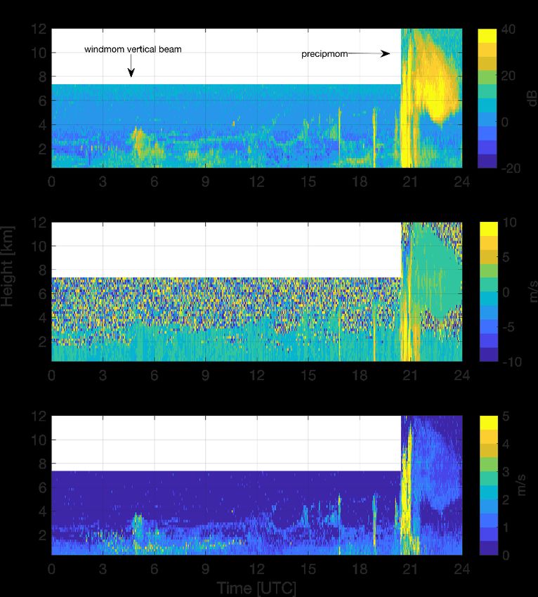
P Muradyan and R Coulter, March 2020, DOE/SC-ARM-TR-044

5.1.3 Precipitation Operation

Along with the wind mode operation when the RWPs cycle through oblique and vertical beams (at least
three beams are necessary for wind determination), the four RWPs at the SGP Central and Intermediate
Facilities operate in a precipitation mode in conjunction with cloud scanning radars. In this mode, the
RWPs transmit only in the vertical direction with shorter averaging times and larger spectral domains. In
this mode they are not able to obtain winds very efficiently. However, they can sample precipitation quite
well up to as high as 16 km. In this case, they measure the fall velocity of rain or snow, relative to the air
motion. In conjunction with some assumptions regarding the relationship between terminal velocity of
water/snow and the spectrum of the fall velocities, updraft/downdraft locations and magnitudes can be
determined. Particularly in parallel with scanning Doppler radar measurements, these measurements can
contribute to a better understanding of in-cloud processes.

Because the wind measurements are compromised by the fall velocities and improved understanding of
in-cloud processes require high-temporal-resolution precipitation measurements, an “adaptive” algorithm
has been implemented at all four SGP sites since 05/2018 to operate only in precipitation mode when
precipitating conditions are identified via real-time monitoring of moments data. Figure 4 shows the SNR,
the vertical velocity, and the spectral width collected with the wind mode up to about 2025 UTC, when
precipitating conditions are identified by the algorithm and the profiler switches to operating in
precipitation mode providing high-temporal-resolution vertical beam low- and high-power measurements.

Figure 4. An example of adaptive algorithm’s operation switching from wind mode to precipitation
 mode only when precipitating conditions have been identified.

 7
P Muradyan and R Coulter, March 2020, DOE/SC-ARM-TR-044

5.2 Data File Contents
The file structures described below are similar for both the wind and precipitation mode operation, with
the precipitation mode only having the vertical component.

5.2.1 Data Types

5.2.1.1 Wind Profile Data

 • Spectral Data
 – At each height, beam pointing direction, and power level:
 ○ Spectral amplitude (at each bin of FFT).
 • Moments Data
 – At each beam pointing direction, and power level:
 ○ At each range gate:
 • Mean Doppler shift (in % of Nyquist frequency)
 • Spectral width (in % of Nyquist frequency)
 • SNR level (in dB)
 • Noise level (in dB)
 • Average Data
 – At each power level:
 ○ At each range gate:
 • Wind speed (in m/s)
 • Wind direction (degrees relative to true north)
 • For each beam pointing direction:
 o Radial wind speed (positive = toward the antenna)
 o Number of moments that passed consensus criteria
 o Average SNR

5.2.1.2 Virtual Temperature Profile Data

 • Spectral Data
 – At each height:
 ○ Spectral amplitude (at selected bins of FFT).
 • Moments Data
 – At each range gate:
 ○ Mean Doppler shift of vertical atmospheric motion (in % of Nyquist frequency)
 ○ Spectral width of vertical atmospheric motion (in % of Nyquist frequency)
 ○ SNR level of atmospheric portion of spectrum (in dB)
 ○ Noise level of atmospheric portion of spectrum (in dB)
 ○ Mean Doppler shift of acoustic signal (in % of Nyquist frequency)
 ○ Spectral width of acoustic signal (in % of Nyquist frequency)
 ○ Noise level of acoustic signal portion of spectrum (in dB)
 ○ SNR level of acoustic signal portion of spectrum (in dB)

 8
P Muradyan and R Coulter, March 2020, DOE/SC-ARM-TR-044 • Average Data o At each height: Virtual temperature (Co) Corrected (for vertical motion) virtual temperature (Co) Vertical wind speed ( in m/s, positive upward) Number of moments that passed consensus criteria for: • Uncorrected virtual temperature • Corrected virtual temperature • Vertical motion SNR (in dB) for: • Uncorrected virtual temperature • Corrected virtual temperature • Vertical motion Additional information may be found in the netCDF file header descriptions for RWP data ordered from the ARM Data Center. 5.2.2 Primary Variables and Expected Uncertainty The primary quantities measured with the RWP system are the intensity and Doppler frequency of backscattered radiation. The wind speed is determined from the Doppler frequency of energy scattered from refractive index fluctuations (caused primarily by moisture fluctuations but also, to a lesser extent, by temperature fluctuations) embedded within the atmosphere; the virtual temperature is determined from the Doppler frequency of microwave energy scattered from acoustic energy propagating through the atmosphere. Definition of Uncertainty The primary observed quantities are Doppler frequency and signal amplitude. Note that the observed quantities above are not the principal quantities of interest to most scientists. The derived quantities of most interest to scientists are the wind speed, wind direction, vertical wind speed, and virtual temperature as a function of height. The accuracies of these quantities, while dependent upon the accuracy of the frequency measurement, are also affected by atmospheric effects and vary considerably according to conditions. The wind speed is derived from measurements from, normally, five beams. Because the individual components are not collocated in space, horizontal homogeneity is assumed to derive the wind vector at a single height. Furthermore, the data are sampled at equal time intervals along each transmit direction. Thus, the vertical beam is sampled at larger height intervals than are the tilted beams (by 1/sin[elevation angle]). This difference is approximately 3%, which can be significant at large ranges. For example, at a nominal height of 1000 m (tilted beams), the vertical beam information is derived from 1035 m, which can be significant in some situations • Nominal accuracy for wind speed: 1 m/s • Nominal accuracy for radial wind components along the pointing direction of the transmitter (e.g., vertical velocity): 0.5 m/s • Nominal accuracy for wind direction: 3o • Nominal accuracy for virtual temp: 0.5 K 9
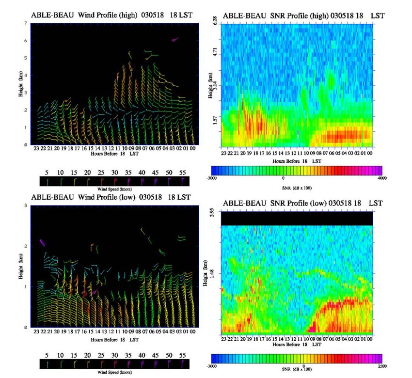
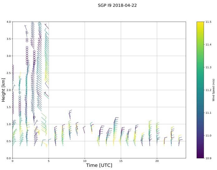
P Muradyan and R Coulter, March 2020, DOE/SC-ARM-TR-044

These figures are the result of more than one year of daily and multi-day comparisons with winds derived
from the balloon-borne sounding system at the Central Facility of the Southern Great Plains observatory.

5.2.3 Data Quality Flags

No flags are applied during the data ingest of the consensus-averaged winds and virtual temperatures.
However, the data are examined regularly by the instrument mentor for quality assurance: files are created
and maintained by the DQO on a monthly basis for each of the instruments that determine locations
(temporally and spatially) where data should be eliminated based on a brute force, multi-pass comparison
with data from neighboring points (above, below, before, and after). This routine eliminates most of the
questionable data. However, several situations defy straightforward objective analysis routines, most of
which can be delineated by subjective analysis. This is done monthly by the instrument mentor. The
primary situations that can create seemingly good, but actually erroneous, data include:
 • Precipitation: Both rain and snow are excellent sources of scatter of electromagnetic radiation; thus,
 they have the potential to provide considerable increases in the effective range for useful data.
 However, precipitation generally has a heterogeneous spatial distribution on the scale of the
 separation of the transmitted beams. This can lead to significant errors in the estimates of the true
 wind speed. Rainfall is more amenable to objective analysis detection because it usually has a large
 downward velocity in comparison to atmospheric motion. Snow, on the other hand, has quite small
 terminal velocities. Figure 5 shows the effect of precipitation on the consensus winds on 2018-04-22
 at the SGP I9 facility. The precipitation lasts up to 0500 UTC, with the peak precipitation at around
 0300-0400 UTC, and is expressed as increased SNR on the left panel extending up to 5 km. During
 this time window while the height coverage of wind profiles is increased, the wind speed estimates,
 especially during peak precipitation times, may be adversely affected.

 Figure 5. Precipitation effect on the consensus winds.

 • Birds: The effects of birds, particularly migrating birds, is both difficult to detect and significant. The
 profiler is sensitive not only to the motion of the bird itself, but to the motion of its wings. During
 migrating seasons (fall and spring), nighttime winds from the north (fall) and south (spring) are often
 affected by these effects. The birds generally fly along the direction of the wind and increase the
 detected wind speed by 5 m/s or more (Coulter and Holdridge 1996, Pekour and Coulter 1998).

 10
P Muradyan and R Coulter, March 2020, DOE/SC-ARM-TR-044

 Figure 6 shows the low- (bottom) and high- (top) power winds (left) and SNR (right) that are affected
 by migrating birds. Note the obvious wind direction shift near 2000 hours local standard time for
 roughly a 5-hour period. In this case, the winds were light enough that the birds flew north anyway. In
 cases when the winds are directly along the direction of the birds’ desired direction of flight, the
 evidence is quite difficult to determine using the wind barb plot alone. Note the “random-type” strong
 reflections around 0.7 km on the low-power SNR. These are characteristic of migrating bird signals.
 Note also that the signature for the high-power returns is considerably different from the low-power
 returns because of the considerably longer transmit pulse duration used. Finally, it can be noted that
 in this case the high-power winds are more affected at lower altitudes than are the low-power winds.
 Obviously, purely objective analysis is difficult in these cases.
 • 60-Hz noise: When 60-Hz noise gets directly into the analyzed Doppler signal it is detected
 approximately as a Doppler shift associated with a radial wind speed of 10 m/s. Because the Nyquist
 frequency for winds is often near 10 m/s, the noise signal is sometimes aliased back into the spectrum
 as well. Depending on which antenna beam is affected, very large deviations in wind speed can occur.
 Some of these are easily removed, but some provide consistent values not completely removed by
 some objective analysis routines. In addition, it reduces the range of accessible data.

Figure 6. Low- (bottom) and high- (top) power winds (left) and SNR (right) affected by migrating
 birds.

 11
P Muradyan and R Coulter, March 2020, DOE/SC-ARM-TR-044

5.3 Annotated Examples.
Examples are provided throughout the handbook.

5.4 User Notes and Known Problems
 • April 9, 1997: A noise peak in the spectra of the intermediate facility profilers located at +/- 60 Hz
 from 0 was reported. This was a relatively serious problem because it effectively raised the minimum
 detectable signal level from -22 dB to -16 dB, a factor of 4. We still do not know the true cause of the
 problem, except that it appeared to be a 60-Hz noise problem. However, actions taken at Beaumont,
 including adjusting, but not changing, the configuration of the ground wires has considerably reduced
 the occurrences of “bad” accepted data due to 60-Hz noise (75 % approximately) and reduced the
 minimum detectable SNR level to about -20 to -21 dB. At Medicine Lodge, maintenance on the phase
 shifter assembly in December 1999 apparently changed the configuration in some minor way so that
 it also is reporting much less “bad” data and has a minimum SNR level near -20 dB. In both cases,
 however, the minimum SNR level is due to the 60-Hz noise. At Meeker, the problem has never been
 quite so severe and has a minimum SNR value near -19 to -20 dB.
 • Spring, 2019: The 1290 MHz Scintec RWP at the Eastern North Atlantic site started demonstrating
 degradation of sensitivity. The Scintec radar engineer evaluated the profiler on site from July 8 to July
 12, concluding that the antenna and the phase shifter are dramatically affected by heavy corrosion and
 cannot be repaired. The profiler will become operational again after the purchase and installation of
 new components.
 • October 14, 2019: A noise peak in the spectra at the SGP I10 facility located at about +/- 60 Hz from
 0 was noticed. Both internal and external potential sources of interference were considered; thorough
 evaluation of the RWP system components was performed. As a result, it was found that the outdoor
 cables passing through conduit were dramatically affected by the moisture accumulation inside the
 conduit, which was causing the problem.
 • November 2019: During the initial setup and data validation stage of the Cold-Air Outbreaks in the
 Marine Boundary Layer Experiment (COMBLE) deployment of the AMF1, it was noticed that the
 1290 MHz RWP was not switching beams. Through thorough evaluation of system components it
 was determined that some of the phase shifter relays were not working, while all relays were affected
 by age and corrosion. All phase shifter relays were upgraded for the remainder of COMBLE.

5.5 Frequently Asked Questions
 • Why don’t the profiler values of winds and/or temperature agree with values from the radiosonde
 balloon-borne sounding system (BBSS)?
 – The RWP provides values averaged over (nominally) 1 hour while the BBSS obtains only a grab
 sample at one instant in time at each height.
 – The balloon from the BBSS travels with the mean wind; hence, it is not collocated with
 measurements from the RWP.
 – The RWP values are volume averages over (nominally) 60–240 meters in height by 9 degrees
 horizontally.

 12
P Muradyan and R Coulter, March 2020, DOE/SC-ARM-TR-044

 – The BBSS measures temperature; the RWP measures virtual temperature.
 – The RWP may be detecting birds rather than the true wind.
• What are the factory-recommended calibration procedures?
 The only true calibration procedures are carried out during the Acceptance Test (AT) that is
 performed immediately before the instruments are put into service. These are carried out by the
 vendor and the instrument mentor. They include the following:
 – Output power: Measured at the output of the final amplifier/preamplifier, including both forward
 and reflected power measurements (3990 W and >500 W for 50 MHz and 915 MHz,
 respectively).
 – Center frequency: Transmit frequency (49.8 MHz and 915 MHz for the 50 MHz and 915 MHz
 RWPs respectively) is measured using a signal generator input to the receiver.
 – Doppler direction: Using a special control parameter file, small signal frequency differences are
 analyzed to determine the appropriate sign of the analyzed frequency difference.
 – Dynamic range: A signal generator with variable attenuator is used as input to the system to
 establish a dynamic range of at least 55 dB.
 – System sensitivity: A signal generator is used to establish a minimum detectable level of at least
 -127 dBm.
 – Range verification: A delay line is used to establish range accuracy of +/- 30 m.
• What are the factory-recommended performance checks?
 These include visual inspection, system power, timing, data transfer, antenna integrity, and RASS (if
 applicable) operation verification. Additional performance checks suggested by the vendor include:
 – Control lights
 – Date and time accuracy
 – Final Amplifier current stationary
 – Appropriate antenna rotation
 – Data appearance
 – SNR levels unchanged
• What are the mentor calibration procedures?
 – There are no “mentor calibration procedures” other than comparison of data with other available
 sources of data. This, however, is more of a QC check.
• What are the mentor performance checks?
 – Regular noise level checks
 – Regular final amplifier current checks
 – Daily data existence
 – Inspection of vertical time section of winds/temperatures and moments

 13
P Muradyan and R Coulter, March 2020, DOE/SC-ARM-TR-044

 – Continuous (daily) maximum height attained monitoring
 • What is the standard schedule of calibrations and checks, and is any data affected or lost during the
 procedures?
 – Factory calibrations are done at the time of installation. All data during the basic factory
 calibration, that 1−2 days, is lost.
 – Other checks are designed for site operators to perform (daily, monthly and yearly preventative
 maintenance). No data is affected/lost during these checks.
 • Does storage media exist on the instrument system to back up data and store it for delayed data
 ingest?
 – The hard disk can hold spectra and consensus files for approximately 12 days. It can hold
 consensus-only data for 1 year. An optical disk can hold spectral data for 12 months.

6.0 Data Quality
 As with all ARM instruments, data quality is a critical issue for RWP and RASS units.

 6.1 Data Quality Health and Status
 The Data Quality Office website has links to several tools for inspecting and assessing RWP data quality:

 • DQ Explorer
 • DQ Plot Browser
 • NCVweb: Interactive web-based tool for viewing ARM data.

 The tables and graphs shown contain the techniques used by ARM data quality analysts, instrument
 mentors, and site scientists to monitor and diagnose data quality.

 6.2 Data Reviews by Instrument Mentor
 • Quality control (QC) frequency: Daily
 • QC delay: Instantaneous; daily
 • QC type: Min/max flags, graphical plots, intercomparisons
 • Inputs: Raw data
 • Outputs: Summary reports

 Data QC procedures for this system are mature.

 1. Data flags:
 A procedure used to be in place for several years that produced a parallel datastream to
 the “.a2” data, which consists of consensus-averaged wind and temperature profiles
 produced by the wind profiler. These data are unchanged from the original data but have

 14
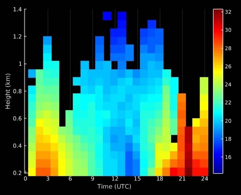
P Muradyan and R Coulter, March 2020, DOE/SC-ARM-TR-044

 an additional data field consisting of flags referring to data that are questionable. The
 flags were determined based on differences between successive wind or temperature
 variables. Comparisons are made both in time and space and both forward and backward
 (i.e., comparisons with previous and successive values at a given height as well as
 comparisons with values above and below at a given time.) If the values exceed defined
 limits, they are flagged.
 2. Comparison with radiosonde data:
 Every routine launch of radiosondes by the BBSS used to be compared in wind speed,
 wind direction, and virtual temperature between the BBSS and the 50 MHz and 915 MHz
 profilers at the Central Facility. The approach taken was to compare all values of “good”
 profile values with BBSS values averaged over nearly the same height interval. The
 differences are used to produce the mean, standard deviation, maximum, minimum, and
 number of values. These data are appended to a file that dates back to June 20, 1995.
 Summary plots of these data are inspected to determine degraded system performance
 (Coulter and Lesht 1997). The statistics of the differences were inspected daily.
 3. Estimated maximum height of return:
 The daily data from 915 MHz wind profilers are used to determine the maximum height
 attained in at least 25%, 50%, and 75% of the profiles during each 24-hour period. These
 data are appended to a file (for each site) beginning January 25, 1993 (915 MHz at CF),
 March 24, 1994 (50 MHz at CF), and January 1, 1997 (915 MHz at intermediate
 facilities). These data are plotted occasionally to determine trends that might indicate
 hardware problems.
 4. Daily inspection:
 Vertical time sections of hourly averaged wind and temperature profiles over a 24-hour
 period are visually inspected on a daily basis for system and operation consistency.

6.3 Data Assessments by Site Scientist/Data Quality Office
All DQO and most site scientist techniques for data assessment have been incorporated within
DQ Explorer.

6.4 Value-Added Products
Many of the scientific needs of the ARM user facility are met through the analysis and processing of
existing data products into value-added products (VAPs). Despite extensive instrumentation deployed at
the ARM sites, there will always be quantities of interest that are either impractical or impossible to
measure directly or routinely. Physical models using ARM instrument data as inputs are implemented as
VAPs and can help fill some of the unmet measurement needs of the ARM facility. Conversely, ARM
produces some VAPs, not to fill unmet measurement needs, but to improve the quality of existing
measurements. In addition, when more than one measurement is available, ARM also produces
“best-estimate” VAPs. For more information see https://www.arm.gov/capabilities/vaps.

 15
P Muradyan and R Coulter, March 2020, DOE/SC-ARM-TR-044

7.0 Instrument Details

 7.1 Detailed Description

 7.1.1 List of Components

 The 915-MHz and 1290-MHz radar wind profilers are manufactured by Vaisala Corp. They comprise a
 single-phased microstrip antenna array consisting of nine “panels” (most systems have only four panels).
 The antenna is approximately 4-m square and is oriented in a horizontal plane so the “in-phase” beam
 travels vertically. Below is a list of components for these RWPs:
 • Antenna assembly, including the clutter fence
 • Computer, including the radar processing unit
 • Final Amplifier (FA)
 • Modulator, Intermediate Frequency and Interface unit (MII)
 • Phase shifter
 • FA power supply.

 The 1290-MHz beam-steered RWP (BSRWP) is manufactured by DeTect, Inc. It has phase control over
 each of the 64 discrete elements to enable beam pointing on a pulse-by-pulse basis. Below is a list of
 components for the BSRWP:
 • Antenna assembly, including the clutter fence
 • Computer, including the radar processing unit
 • High-power amplifier
 • GPS compass, including a 3-GPS antenna receiver system and an Inertial Measurement Unit (IMU)
 • Transmit/Receive switch
 • Profiler health monitor
 • Intermediate Frequency Conditioner.

 7.1.2 System Configuration and Measurement Methods

 The radar wind profilers operate by transmitting in two different vertical planes and receiving
 backscattered energy from refractive index fluctuations that are moving with the mean wind. By sampling
 in the vertical direction and in two tilted planes, the three components of motion can be determined. The
 systems (Vaisala and Scintec) consist of a single-phased array antenna that transmits alternately up to five
 pointing directions: one vertical, two in the north-south vertical plane (one south of vertical, one north of
 vertical), and two in the east-west vertical plane (one east of vertical, one west of vertical). The
 non-vertical beams are tilted at about 14o from vertical.

 16
P Muradyan and R Coulter, March 2020, DOE/SC-ARM-TR-044

Radial components of motion along each pointing direction are determined sequentially. It takes,
nominally, 30-45 seconds (dwell time) to determine the radial components from a single pointing
direction. Thus, at the SGP site the system currently cycles through three beams (two obliques and
vertical) at low power, and then cycles the three beams again at a high-power (longer pulse length)
setting. Then the whole process is repeated. About three minutes elapse before the system returns to the
beginning of its sequence. Within an averaging interval, the estimates from each beam-power
combination are saved; these values are examined and compared at the end of the period to determine the
consensus-averaged radial components of motion.

Consensus averaging consists of determining if a certain percentage (e.g., 50 %) of the values fall within a
certain range of each other (e.g., 2 m/s). If they do, those values are averaged to produce the radial wind
estimate. The radial values are then combined to produce the wind profile. The results of this averaging
process are what are reported in the “.a2” data files produced by the ARM data system. Included in these
files are height, speed, direction, radial components, number of values in consensus, and SNR.

During a single time period over which the system operates in a single pointing direction (dwell time), the
data that are produced in the “.a1” and “.a0” files are created. The system transmits pulses at about
1–10 kHz rate into the atmosphere. The backscatter from each transmit pulse is sampled at, for example, a
1 MHz rate. This results in 1 sample every 150 minutes in range. The samples at each range gate are
averaged together (time domain integration) over some number (e.g., 100) of pulses to produce a phase
value for input into a FFT. After (e.g., 64) values are produced, the FFT is performed (one for each range
gate). This process takes on the order of one second. A number (about 30) of these spectra are then
averaged together during the dwell time. At the end of the dwell time we have produced a single averaged
spectrum from each range gate along the designated pointing direction. The spectra themselves are placed
in the “.a0” data files.

The spectra are analyzed by the system before moving to the next pointing direction. This analysis
produces estimates of the SNR, the noise, the mean velocity (proportional to frequency), and the spectral
width at each range gate. This is the information that is stored in the “.a1” data files. Both the “.a1” and
“.a0” data files thus have information at about same (dwell time) intervals; however, the data sequences
vary among pointing directions and output powers.

A note of warning about the mean values in the “.a1” files. The values are in % of full scale times 100,
where full scale is the Nyquist velocity of the spectrum. Thus, velocity estimates are determined by
multiplying the “mdf” column by the “oband” or “vband” values (described in the metadata) and dividing
by 10,000.

RASS operation is essentially the same, except that the averaging time is about 10 minutes and only a
single pointing direction (vertical) is used. Also, the atmosphere is “seeded” with a sound wave; the index
of refraction changes created by the sound wave are the signal source. To sample both the sound wave
(speed about 340 m/s) and the atmosphere (to remove air velocity from temperature estimates), a larger
FFT is required (2048 points). This requires a smaller number of points for each time domain integration
and increases the processor time required to calculate the FFT. The “.a0” files again are spectra; however,
only a portion of the spectra are reported, namely a region near 0 Doppler shift to account for atmospheric
motions and a region around the expected speed of sound. The “.a1” files now consist of moments and
widths from both the atmospheric portion of the spectrum and from the acoustic portion (the main
contributor to the temperature calculation). The “.a2” files consist of profiles of temperature and number
of consensus values.

 17
P Muradyan and R Coulter, March 2020, DOE/SC-ARM-TR-044

7.1.3 Specifications

 • Frequency: 915 or 1290 MHz
 • Maximum range: 3–6 km (16 km for precipitation detection)
 • Range gate: 0.06–1 km
 • Pulse length: 60, 100, 200, 400 m
 • Number of spectra per average spectrum: 1-100
 • Number of pulse/time domain integrations: 1-1000

7.2 Operation and Maintenance

7.2.1 User Manual

A user manual is available to the mentor for the RWPs, with one copy kept at each site.

7.2.2 Routine and Corrective Maintenance Documentation

Routine preventative maintenance procedures (weekly, monthly, yearly) as well as a corrective
maintenance procedure are designed by the mentor for the site operators to perform. These include
factory-recommended procedures (preventative and corrective) for inspecting the antenna, clutter screen,
cables and electronics. ARM operations maintains the corrective maintenance records in an online
database.

7.2.3 Software Documentation

Software documentation provided by the vendors is maintained by the mentor and is also available to the
site operators on the instrument computer.

7.3 Glossary
See the ARM Glossary.

7.4 Acronyms
See the ARM Acronyms.

 18
P Muradyan and R Coulter, March 2020, DOE/SC-ARM-TR-044

8.0 Citable References
 Angevine, WM, and JI MacPherson. 1995. “Comparison of Wind Profiler and Aircraft Wind
 Measurements at Chebogue Point, Nova Scotia.” Journal of Atmospheric and Oceanic Technology
 12(2): 421–426, https://doi.org/10.1175/1520-0426(1995)0122.0.CO;2

 Cohn, SA, and WM Angevine. 2000. “Boundary layer height and entrainment zone thickness measured
 by lidars and wind-profiling radars.” Journal of Applied Meteorology 39(8): 1233−1247,
 https://doi.org/10.1175/1520-0450(2000)0392.0.CO;2

 Ecklund WL, DA Carter, and BB Balsley. 1988. “A UHF Wind Profiler for the Boundary Layer: Brief
 Description and Initial Results.” Journal of Atmospheric and Oceanic Technology 5(3): 432–441,
 https://doi.org/10.1175/1520-0426(1988)0052.0.CO;2

 Ecklund WL, DA Carter, BB Balsley, PE Currier, JL Green, BL Weber, and KS Gage. 1990. “Field Tests
 of a Lower Tropospheric Wind Profiler.” Radio Science 25(5): 899–906,
 https://doi.org/10.1029/RS025i005p00899

 May, PT, and JM Wilczak. 1993. “Diurnal and seasonal variations of boundary-layer structure observed
 with a radar wind profiler and RASS.” Monthly Weather Review 121(3): 673−682,
 https://doi.org/10.1175/1520-0493(1993)1212.0.CO;2

 Merritt, DA. 1995. “A Statistical Averaging Method for Wind Profiler Doppler Spectra.” Journal of
 Atmospheric and Oceanic Technology 12(5): 985–995, https://doi.org/10.1175/1520-
 0426(1995)0122.0.CO;2

 Nastrom, GD, and FD Eaton. 1995. “Variations of Winds and Turbulence seen by the 50-MHz Radar at
 White Sands Missile Range, New Mexico.” Journal of Applied Meteorology 34(10): 2135–2148,
 https://doi.org/10.1175/1520-0450(1995)0342.0.CO;2

 Rogers, RR, D Baumgardner, SA Ethier, DA Carter, and WL Ecklund. 1993. “Comparison of raindrop
 size distributions measured by radar wind profiler and by airplane.” Journal of Applied Meteorology
 32(4): 694−699, https://doi.org/10.1175/1520-0450(1993)0322.0.CO;2

 Weber, BL, and DB Wuertz. 1990. “Comparison of rawinsonde and wind profiler radar measurements.”
 Journal of Atmospheric and Oceanic Technology 7(1): 157−174, https://doi.org/10.1175/1520-
 0426(1990)0072.0.CO;2

 Wilczak, JM, RG Strauch, FM Ralph, BL Weber, DA Merritt, J Jordan, D Wolfe, LK Lewis, DB Wuertz,
 JE Gaynor, S Mclaughlin, RR Rogers, AC Riddle, and TS Dye. 1995. “Contamination of Wind Profiler
 Data by Migrating Birds: Characteristics of Corrupted Data and Potential Solutions.” Journal of
 Atmospheric and Oceanic Technology 12(3): 449–467, https://doi.org/10.1175/1520-
 0426(1995)0122.0.CO;2

 Williams, CR, WL Ecklund, and KL Gage. 1995. “Classification of Precipitating Clouds in the Tropics
 Using 915-MHz Wind Profilers.” Journal of Atmospheric and Oceanic Technology 12(5): 1996–1012,
 https://doi.org/10.1175/1520-0426(1995)0122.0.CO;2

 19
P Muradyan and R Coulter, March 2020, DOE/SC-ARM-TR-044

9.0 Bibliography
 Coulter, RL, and DJ Holdridge. 1995. A three-month comparison of hourly winds and temperatures from
 co-located 50-MHz and 915-MHz RASS profilers. ANL/ER/CP-85219; CONF-9503104-4. Argonne
 National Laboratory, Illinois.

 Coulter, RL, and BM Lesht. 1997. “Results of an automated comparison between winds and virtual
 temperatures from radiosonde and profilers.” In Proceedings of the 6th Atmospheric Radiation
 Measurement (ARM) Science Team Meeting, (pp. 59−60) U.S. Department of Energy.

 Gage, KS, and BB Balsley. 1978. “Doppler radar probing of the clear atmosphere.” Bulletin of the
 American Meteorological Society 59(9): 1074-1094, https://doi.org/10.1175/1520-
 0477(1978)0592.0.CO;2

 Hildebrand, PH, and RS Sekhon. 1974. “Objective determination of the noise level in Doppler spectra.”
 Journal of Applied Meteorology 13(7): 808−811, https://doi.org/10.1175/1520-
 0450(1974)0132.0.CO;2

 Pekour, MS, and RL Coulter. 1999. “A technique for removing the effect of migrating birds in 915-MHz
 wind profiler data.” Journal of Atmospheric and Oceanic Technology 16(12): 1941-1948,
 https://doi.org/10.1175/1520-0426(1999)0162.0.CO;2

 20
You can also read