Rain radar observations of clouds and precipitation - ESSD
←
→
Page content transcription
If your browser does not render page correctly, please read the page content below
Earth Syst. Sci. Data, 14, 33–55, 2022
https://doi.org/10.5194/essd-14-33-2022
© Author(s) 2022. This work is distributed under
the Creative Commons Attribution 4.0 License.

        EUREC4 A’s Maria S. Merian ship-based cloud and micro
          rain radar observations of clouds and precipitation
        Claudia Acquistapace1 , Richard Coulter2 , Susanne Crewell1 , Albert Garcia-Benadi3,4 , Rosa Gierens1 ,
                    Giacomo Labbri6 , Alexander Myagkov5 , Nils Risse1 , and Jan H. Schween1
        1 Institutefor Geophysics and Meteorology, University of Cologne, Pohligstrasse 3, 50969 Cologne, Germany
                       2 Argonne National Laboratory, 9700 S Cass Ave, Lemont, IL 60439, United States
                3 Department Applied Physics–Meteorology, Universitat de Barcelona, Barcelona, 08028, Spain
                            4 Universitat Politècnica de Catalunya, Vilanova i la Geltrú, 08800, Spain
               5 RPG Radiometer Physics GmbH, Werner-von-Siemens-Straße 4, 53340 Meckenheim, Germany
                                 6 Università di Bologna, Via Zamboni 33, 40126 Bologna, Italy

                          Correspondence: Claudia Acquistapace (cacquist@meteo.uni-koeln.de)

                                   Received: 5 August 2021 – Discussion started: 10 August 2021
                      Revised: 19 November 2021 – Accepted: 22 November 2021 – Published: 10 January 2022

       Abstract. As part of the EUREC4 A field campaign, the research vessel Maria S. Merian probed an oceanic
       region between 6 to 13.8◦ N and 51 to 60◦ W for approximately 32 d. Trade wind cumulus clouds were sampled
       in the trade wind alley region east of Barbados as well as in the transition region between the trades and the
       intertropical convergence zone, where the ship crossed some mesoscale oceanic eddies. We collected continuous
       observations of cloud and precipitation profiles at unprecedented vertical resolution (7–10 m in the first 3000 m)
       and high temporal resolution (1–3 s) using a W-band radar and micro rain radar (MRR), installed on an active
       stabilization platform to reduce the impact of ship motions on the observations. The paper describes the ship
       motion correction algorithm applied to the Doppler observations to extract corrected hydrometeor vertical veloc-
       ities and the algorithm created to filter interference patterns in the MRR observations. Radar reflectivity, mean
       Doppler velocity, spectral width and skewness for W-band and reflectivity, mean Doppler velocity, and rain rate
       for MRR are shown for a case study to demonstrate the potential of the high resolution adopted. As non-standard
       analysis, we also retrieved and provided liquid water path (LWP) from the 89 GHz passive channel available on
       the W-band radar system. All datasets and hourly and daily quicklooks are publically available, and DOIs can be
       found in the data availability section of this publication. Data can be accessed and basic variables can be plotted
       online via the intake catalog of the online book “How to EUREC4 A”.

1   Introduction                                                   panded towards additional research questions, extending the
                                                                   campaign area and the number of scientific platforms in-
                                                                   volved. To understand the factors influencing rain forma-
Clouds and precipitation in the tropics are crucial for radia-     tion, study the evolution of mesoscale oceanic eddies and
tive budget and are responsible for climate prediction un-         their impact on air–sea interactions, and produce a dataset
certainties (Bony and Dufresne, 2005). From 19 January to          that can stand as a benchmark for future model evalua-
19 February 2020, the “EUREC4 A: A Field Campaign to               tions and satellite retrievals became complementary goals
Elucidate the Couplings Between Clouds, Convection and             of the enlarged campaign. Within EUREC4 A, the Ocean-
Circulation” campaign (Bony et al., 2017) took place in            Atmosphere component (EUREC4 A-OA, https://eurec4a.eu/
the Atlantic waters southeast of Barbados to test hypothe-         overview/eurec4a-oa/, last access: 18 December 2021) was
ses on trade wind cumuli cloud feedbacks. Stevens et al.           granted two research vessels (R/Vs) in the Atlantic sea south-
(2021) describe how the campaign’s initial scope greatly ex-

Published by Copernicus Publications.
34                                  C. Acquistapace et al.: EUREC4 A’s cloud and micro rain observations from R/V Merian

east of Barbados to monitor the oceanic processes induced by       mpg.de/MCO/ck.html, last access: 18 December 2021), that
large-scale oceanic eddies.                                        is a 250 m3 balloon able to fly up to 2500 m for in situ ob-
   The R/V Maria Sybilla Merian (MS Merian) was deployed           servations of cloud and raindrop size distributions; 3D wind
in the southern part of the EUREC4 A domain to investi-            profiles; and eddy dissipation rates. When combining the W-
gate how mesoscale oceanic eddies impact oceanic circula-          band radar and the co-located in situ observations from the
tion and their role in cloud and precipitation formation. The      cloud kite, a detailed description of the precipitation process
collaboration with the ARM Mobile Facility 2 (https://www.         and unique reference data for high-resolution model runs
arm.gov/capabilities/observatories/amf, last access: 20 De-        become available. The high vertical (7–10 m) and tempo-
cember 2021) equipped the R/V with a comprehensive suite           ral (1–3 s) resolution adopted by all the active remote sens-
of remote sensing instrumentation that could track each stage      ing instrumentation below 2500 m will constitute an essen-
of the precipitation life cycle. A micro rain radar (MRR) and      tial benchmark for future satellite missions like EarthCARE
a cloud radar (W-band) were installed on a stabilization plat-     (Illingworth et al., 2015), providing a detailed description of
form: while the W-band radar is sensitive to a wide range of       the atmospheric layer closer to the surface that is and will
atmospheric scatterers from tiny cloud drops to raindrops, the     be the most critical region to detect from satellites (Lamer
MRR can adequately describe the sub-cloud layer’s rain evo-        et al., 2020). The 1-month precipitation data collected dur-
lution. The 89 GHz passive channel available in the W-band         ing the campaign also represent a vital evaluation dataset
radar system allowed us to characterize the columnar amount        for Global Precipitation Measurement (GPM) mission per-
of liquid water, and integrated water vapor was retrieved only     formance at sea in the subtropics for shallow convection
in clear-sky conditions by means of a linear regression with       precipitation (Hou et al., 2014). The stabilization platform
co-located radiosoundings. All W-band and MRR radar vari-          worked for approximately 65 % of the time, while for 35 %
ables are listed in Sect. 2.1 and 2.2.                             of the time it did not, and we considered ship motion cor-
   The collaboration with ARM and the use of their stabiliza-      rections for both situations. Similar methods have been de-
tion unit allowed the compensation for ship motion and for         rived for airplane-based measurements with Doppler mea-
the first time made it possible to obtain essential Doppler ob-    surements (see, e.g., Bange et al., 2013). The track followed
servations at unprecedented spatial and temporal resolution        by the R/V MS Merian allows us to characterize the latitu-
of the entire precipitation life cycle.                            dinal dependency on the cloud fields when moving from the
   This radar suite represents one of the most advanced re-        subtropics towards the inter-tropical convergence zone and
mote sensing setups for measuring trade wind precipitation         understand the impact of the sea surface temperature hetero-
in and below the cloud. Ground-based cloud radar remote            geneities on the boundary layer (Laxenaire et al., 2018). We
sensing has been used for a long time to monitor the verti-        collected some lessons learned during the EUREC4 A cam-
cal structure of clouds and precipitation (Bretherton et al.,      paign with the hope of encouraging and facilitating future
2010; Lamer et al., 2015; Leon et al., 2008; Kollias et al.,       deployments of active remote sensing instruments on ships,
2007), as well as on ships (Zhou et al., 2015). In recent years,   given the strategic importance that such data might have.
the potential of new observables like the Doppler spectra’s           The paper is organized as follows. Section 2 describes the
skewness to detect precipitation forming in the cloud (Kol-        experimental setup and the instrument characteristics. Sec-
lias et al., 2011b, a; Luke and Kollias, 2013; Acquistapace,       tion 3 provides details on the data processing and on the re-
2017) was demonstrated for fixed ground-based sites. How-          moval of the interference pattern from the data, assessing the
ever, shipborne cloud radar Doppler measurements have not          impact of the ship motion correction algorithm. Section 4 de-
been exploited yet. A first analysis of the unique dataset         scribes a case study of trade wind cumulus clouds and pre-
of trade wind cumulus clouds and precipitation collected           cipitation. We describe how to access data and processing
with the MRR and the W-band radar on MS Merian is pre-             scripts in Sect. 5, while Sect. 6 briefly collects the lessons
sented. Considering typical sea wave periods of 9 s, to obtain     learned and Sect. 7 summarizes the work.
Doppler observations at sea, integration times have to be cho-
sen shorter than 1 s (Chris Fairall, personal communication,
2020). In the paper, we document how specific choices on           2   Experimental setup and data processing
the integration times of the instruments were made, describ-
ing the measurement sampling strategy regarding spatial and        We positioned the radar equipment on the R/V’s top deck at
temporal resolution.                                               around 20 m above sea level, as far as possible from the in-
   The synergistic usage of the dataset collected on the           fluence of sea spray (Fig. 1). The W-band radar and the MRR
R/V will be crucial for tackling precipitation life cycle de-      were mounted on the stabilization platform using two metal
tection using a multiscale approach based on the additional        bars. To limit vibrations, we installed rigid support between
measurements on board not presented here: a water vapor            the MRR’s pole and the W-band radar. At installation, we
Raman lidar and a wind lidar from the University of Hohen-         synchronized the internal clocks of the computers controlling
heim; a cloud kite from the Max Planck Institute for Dynam-        the radar equipment with the ship navigation system clock.
ics and Self-Organization of Göttingen (http://www.lfpn.ds.        Despite this effort, the time stamp synchronization suffered

Earth Syst. Sci. Data, 14, 33–55, 2022                                               https://doi.org/10.5194/essd-14-33-2022
C. Acquistapace et al.: EUREC4 A’s cloud and micro rain observations from R/V Merian                                                      35

Figure 1. Instrument deployment on the R/V MS Merian. (a) View of the top deck (so-called Peildeck): the hydraulic unit is visible on the
right in the metal box, connected via multiple cables to the stabilization platform. (b) The MRR (left) and the W-band radar (right) fixed
using two metal bars on the stabilization platform. (c) Position of the instrument deployment with respect to the motion reference unit (MRU)
on the MS Merian: side view (left) and front view (right).

from a drift of the clocks with respect to the Global Position-          2.1   W-band radar
ing System (GPS) time of the ship’s inertial system variable
between 1 and 4 s that we had to consider in the correction              The W-band radar is a frequency-modulated continuous-
of the data for ship motions. From 19 January to 19 Febru-               wave (FMCW) 94 GHz dual-polarization radar equipped
ary 2020, the R/V MS Merian sailed over a vast oceanic re-               with a radiometric channel at 89 GHz and is manufactured
gion spanning from 6 to 13.8◦ N and from 51 to 60◦ W (see                by Radiometer Physics GmbH (RPG), Germany. The small
Fig. 2). We launched 118 radiosondes and collected 38 de-                diameter of its antennas (0.5 m), one to transmit and one to
scents to provide temperature (T ), pressure (P ), and humid-            receive, and its compactness (Table 1) make it a well-suited
ity (q) profiles during the whole campaign (Stephan et al.,              instrument to be deployed in complex environments. Küch-
2021). This database was used to build a retrieval for inte-             ler et al. (2017) provided an extended description of the radar
grated water vapor from the single passive 89 GHz channel                performance, hardware, calibration, and signal-processing
available on the W-band radar. In the following, we will first           procedures. We calibrated the receiver of the W-band radar
describe the two radars followed by the stabilization plat-              after installing it in the position shown in Fig. 1. To pro-
form, and we will describe the motion reference unit (MRU)               tect the hydrophobic radome from hydrometeors, the radar
and the ship reference system.                                           is equipped with a blower for both antennas. The blower is
                                                                         able to produce a thin airflow with up to 20 m s−1 over the an-
                                                                         tenna radomes (Küchler et al., 2017). Users can set different

https://doi.org/10.5194/essd-14-33-2022                                                        Earth Syst. Sci. Data, 14, 33–55, 2022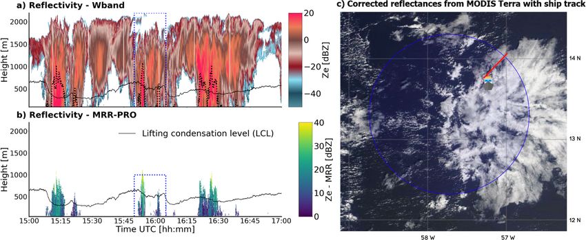
36                                  C. Acquistapace et al.: EUREC4 A’s cloud and micro rain observations from R/V Merian

                                                                  tions and one ERA-Interim reanalysis column (Dee et al.,
                                                                  2011). For more details on the ANN and the dataset used for
                                                                  it, please refer to Appendix A and Table A1.
                                                                      We obtained integrated water vapor (IWV) estimates by
                                                                  applying a single-channel retrieval in clear-sky cases, defined
                                                                  as profiles where all W-band radar reflectivity values are
                                                                  smaller than −50 dBz. The retrieval is based on the quadratic
                                                                  regression between the 89 GHz brightness temperatures and
                                                                  the IWV estimated with the radiosoundings. We selected all
                                                                  radiosoundings with relative humidity smaller than 97 % in
                                                                  the entire profile launched when no cloud base was detected
                                                                  by the wind lidar on board MS Merian. The IWV results from
                                                                  integrating the profile of specific humidity over height and is
                                                                  associated with the mean 89 GHz brightness temperature cal-
Figure 2. Ship track of the R/V MS Merian during the EUREC4 A     culated over 1 min after the radiosonde launch.
campaign, from 19 January to 19 February 2020.                        The W-band radar data collected during the EUREC4 A
                                                                  campaign have been post-processed using a software pack-
                                                                  age that includes processing and de-aliasing of compressed
range resolutions at different altitudes by providing the nec-    and polarized spectra. The code is an update and a subse-
essary parameters to the so-called “chirp table”, i.e., a table   quent restructuring of the first program version provided by
storing all the frequency modulation settings. Table 2 shows      Küchler et al. (2017), and it is available at https://github.com/
the chirp table definition adopted for this measurement cam-      igmk/w-radar/tree/new_output_structure (last access: 23 De-
paign. We defined the chirp table to have a high vertical reso-   cember 2021). No liquid attenuation correction has been ap-
lution below the inversion layer to focus on shallow cumulus      plied to the data yet. The post-processing routine produces as
clouds (Table 2). This choice resulted in reaching a maxi-        output a technical data file including all radar specific vari-
mum detectable range of 10 000 m to focus on high vertical        ables and a physical data file, available in two versions. One
resolution of the boundary layer clouds and the inability to      version (compact), structured as daily files, includes
measure high cirrus clouds. The range resolution from the
sea level to 1233 m was 7.5 m, while it was 9.2 m between           – radar moments (equivalent reflectivity factor (from now
1233 and 3000 m. Between 3000 and 10 000 m the range res-             on called reflectivity), mean Doppler velocity negative
olution was 34.1 m. We chose integration times of 0.846 s             towards the ground, Doppler spectral width, Doppler
for heights smaller than 1233 m, 0.786 s between 1233 and             spectrum skewness, Doppler spectrum kurtosis);
3000 m, and 1.124 s between 3000 and 10 000 m to make the           – coordinates (time, height, latitude, longitude);
ship motion correction effective. The total sampling time re-
quired to measure a full profile resulted in around 3 s.            – integrated variables (liquid water path, brightness tem-
   The embedded passive channel operates at 89 GHz with               perature at 89 GHz);
a bandwidth of 2 GHz and measures the calibrated bright-
ness temperature (TB). In the W-band, atmospheric gases             – surface variables collected by the meteo station attached
are relatively transparent. The absorption coefficient of at-         to the radar (wind speed and direction, pressure, temper-
mospheric gases in the lower troposphere is of the order              ature, rainfall rate, and humidity);
of 1 dB km−1 (Ulaby et al., 1981). In contrast, cloud liquid        – general parameters (file code/version number, compres-
water produces a strong attenuation (≈ 1 dB km−1 g−1 m3 ;             sion flag).
Ulaby et al., 1981) in this frequency band. Since the passive
measurements are sensitive to the presence of liquid water,       The other version (complete radar data), organized in hourly
the TB measured at 89 GHz can be used in a retrieval of           files, includes all the previous variables plus additional radar
liquid water path (LWP) (Küchler et al., 2017). The cloud         variables like the Doppler spectrum, the bin mean noise
radar continuously runs a statistical retrieval developed by      power, and the sensitivity limit. In addition to the standard
the radar manufacturer. The retrieval is based on an artifi-      processing, we derived and added the mean Doppler veloc-
cial neural network (ANN), which approximates values of           ity field corrected for ship motions to the variables listed
LWP for a given set of the observed TBs, surface tempera-         above in both versions of the files. The compact version
ture, relative humidity, pressure, and day of the year. For the   has been enhanced with Climate and Forecast (CF) con-
ANN training, a dataset of atmospheric profiles was used.         ventions (https://cfconventions.org/, last access: 23 Decem-
Since the ship was moving around Barbados during the cam-         ber 2021) to allow online plotting using the EUREC4 A book
paign, data from several surrounding stations were combined       (https://howto.eurec4a.eu/intro.html, last access: 23 Decem-
in the dataset. The dataset consisted of three radiosonde sta-    ber 2021). Section 3.1 and 3.2 describes the post-processing

Earth Syst. Sci. Data, 14, 33–55, 2022                                               https://doi.org/10.5194/essd-14-33-2022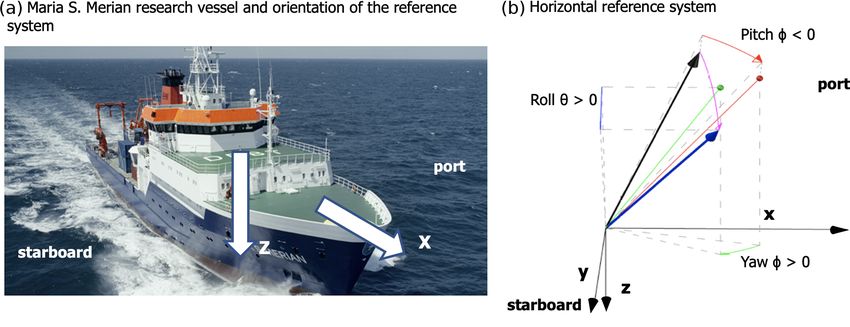
C. Acquistapace et al.: EUREC4 A’s cloud and micro rain observations from R/V Merian                                                 37

Table 1. Instruments’ technical specifications.

                           Parameter name                    MRR-PRO                  W-band
                           Operating frequency (GHz)         24.23                    94
                           Operating mode                    FMCW                     FMCW
                           Modulation (MHz)                  0.5–15                   up to 100
                           Transmit power (W)                0.05                     1.5
                           Antenna diameter (m)              0.6                      0.5
                           No. of range gates                128                      550
                           Range resolution (m)              10                       7.5, 9.2, and 34.1
                           Resulting measuring range (m)     0–1270                   100–10 000
                           Temporal resolution (s)           1 (10 on some days)      3
                           Beam width (two-way, 6 dB)        1.5◦                     0.48◦
                           Nyquist velocity range (m s−1 )   ±6.0 (0 to 11.9)         10.8, 7.3, and 5.1
                           No. of spectral bins              64                       1024, 256, and 256
                           Spectral resolution (m s−1 )      0.1889                   0.0415, 0.0569, and 0.0398
                           Power (W)                         500                      400 (radar), 1000 (blower)

Table 2. Chirp table definition for W-band radar.

                              Attributes                                         Chirp sequence (CS)
                                                                         CS 1            CS 2             CS 3
                              Integration time (s)                      0.846           0.786           1.124
                              Range interval (m)                     100–1233       1233–3000     3000–10 000
                              Range vertical resolution (m)                7.5             9.2            34.1
                              Nyquist velocity (m s−1 )                   10.8             7.3              5.1
                              Doppler velocity bins                       512             256              256
                              Doppler velocity resolution (m s−1 )     0.0415          0.0569          0.0398

applied to the data, and Sect. 5 explains the available data            the interference filter are provided in Sect. 3.2 and 3.4, re-
products.                                                               spectively. Finally, all variables are derived by standard post-
                                                                        processing of the shifted spectra. The variables are reflec-
                                                                        tivity considering only liquid drops, equivalent reflectivity
2.2   Micro rain radar                                                  non-attenuated, equivalent reflectivity attenuated, hydrom-
The micro rain radar (MRR) deployed on the R/V MS Merian                eteor fall speed, spectral width, skewness and kurtosis of
is a vertically pointing frequency-modulated continuous-                the Doppler spectra, liquid water content, rainfall rate, rain
wave (FMCW) Doppler radar operating at 24.23 GHz, pro-                  drop size distribution, raindrop diameter weighted over mean
duced by the Meteorologische Messtechnik GmbH (Metek)                   mass, time, height, latitude, and longitude. Attenuation due
(Peters et al., 2002) and owned by the University of Leipzig.           to precipitation has been taken into account. More details on
The instrument deployed was the latest version of the MRR,              the derivation of the MRR-PRO variables can be found in
the so-called MRR-PRO, with an antenna diameter of 0.6 m                Garcia-Benadi et al. (2020). Files are then structured in daily
(Fig. 1), and comes with a factory calibration. Table 1 con-            files, and CF conventions are applied to make file readability
tains the main technical characteristics of the MRR-PRO                 easier. For the rest of the paper we refer to equivalent reflec-
and the specific settings adopted during the campaign. Dur-             tivity non-attenuated as simply reflectivity.
ing the course, we observed interference of the instrument
with the stabilization platform device. For this reason, we             2.3   ARM AMF-2 stabilization platform
post-processed the data independently instead of relying on
the postprocessing of the manufacturer. Initially the pre-              The stabilization platform from the US Atmospheric
processing converts the Doppler velocity range and performs             Radiation Measurement (ARM) program Mobile Facil-
the de-aliasing. Then, the interference is filtered out. The next       ity 2 (AMF2) was deployed on the R/V MS Merian to reduce
step is to calculate the correction for ship motions for each           the impact of ship motions on the Doppler zenith pointing
time stamp and shift the Doppler spectra of the correction              observations (Coulter and Martin, 2016). The system, built
amount. Details on the ship motion correction algorithm and             by Sarnicola Systems, is an active stabilization system; i.e.,

https://doi.org/10.5194/essd-14-33-2022                                                          Earth Syst. Sci. Data, 14, 33–55, 2022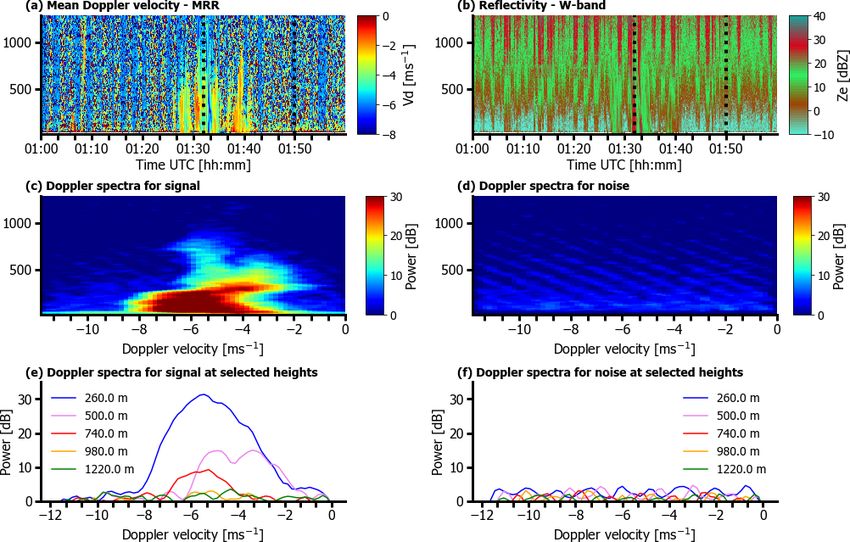
38                                    C. Acquistapace et al.: EUREC4 A’s cloud and micro rain observations from R/V Merian

Figure 3. Time series of (a) heave, (b) roll, (c) pitch, and (d) yaw of the R/V MS Merian MRU unit during the EUREC4 A campaign, from
19 January to 19 February 2020. Grey areas represent the periods of time in which the stabilization platform did not work.

it compensates for the ship motions by adapting the position            relatively calm sea conditions afterwards (Fig. 3). It must be
of the table surface correspondingly so that the radar stays in         noted that the stabilization platform can compensate for the
a zenith pointing position. It requires 120 V power and eth-            rotation of the ship, but it can not compensate for the verti-
ernet connection to a computer in a sealed container to be              cal movements along the vertical axis (e.g., heave) and the
operational. A hydraulic power unit (HPU) (the cubic metal              translations which occur because the ship rotates around its
box on the right in Fig. 1a) must be within 600 cm of the ta-           center of mass while the instruments are located elsewhere
ble and weighs approximately 182 kg. The HPU supplies hy-               (see Sect. 3).
draulic fluid to manipulate the length of three legs positioned
below the table’s surface such that the table can compensate
                                                                        2.4   Motion reference unit (MRU) and ship reference
for a large range of roll and pitch angles of the ship. More
                                                                              system
information on the stabilization platform can be obtained
at https://www.arm.gov/capabilities/instruments/s-table (last           When deploying a radar on a ship, vertical velocity measure-
access: 23 December 2021). Ship and table motion are moni-              ments have to be corrected for ship motions, i.e., roll, pitch,
tored by two roll–pitch sensors, one located on the ship deck           yaw, and heave (Fig. 3). Roll and pitch variations cause the
and the other in the center of the table itself. A predictive           radar beam to be off-zenith and vertical range to vary with
computer routine uses these values to maintain the table in             time, heave variations in time cause a vertical velocity offset
a geopotential level orientation at a constant height above             and the vertical range to vary with time, and the ship drift in
the ship’s surface. Thus the table compensates for the rota-            the horizontal plane described by surge and sway may also
tional motions around the long axis of the ship (roll) and the          have components in the direction of the radar beam if the
short axis of the ship (pitch). Stabilization platform data re-         radar is looking in any direction tilted from the vertical rel-
vealed that the table did not work for approximately 35 % of            ative to ocean. In this work, we will not calculate the surge
the time. The longest interval in which the stabilization plat-         and sway motions because we assume them to be negligible
form was not working occurred between 1 and 5 February,                 compared to the other terms.
when a connection cable was badly damaged and had to be                    All rotation angles are measured by the motion reference
exchanged. Around 17 February, we finally fixed the stabi-              unit (MRU) on the ship with a time resolution of 1 s. The
lization platform, and in the last 2 d the stabilization platform       MRU is a Kongsberg “Seapath 320” system manufactured
worked continuously. Overall, we encountered the roughest               by Kongsberg SeaTex AS. The sensor uses two single-
sea conditions at the beginning of the campaign, and we had             frequency 12-channel GPS receivers for position and head-

Earth Syst. Sci. Data, 14, 33–55, 2022                                                      https://doi.org/10.5194/essd-14-33-2022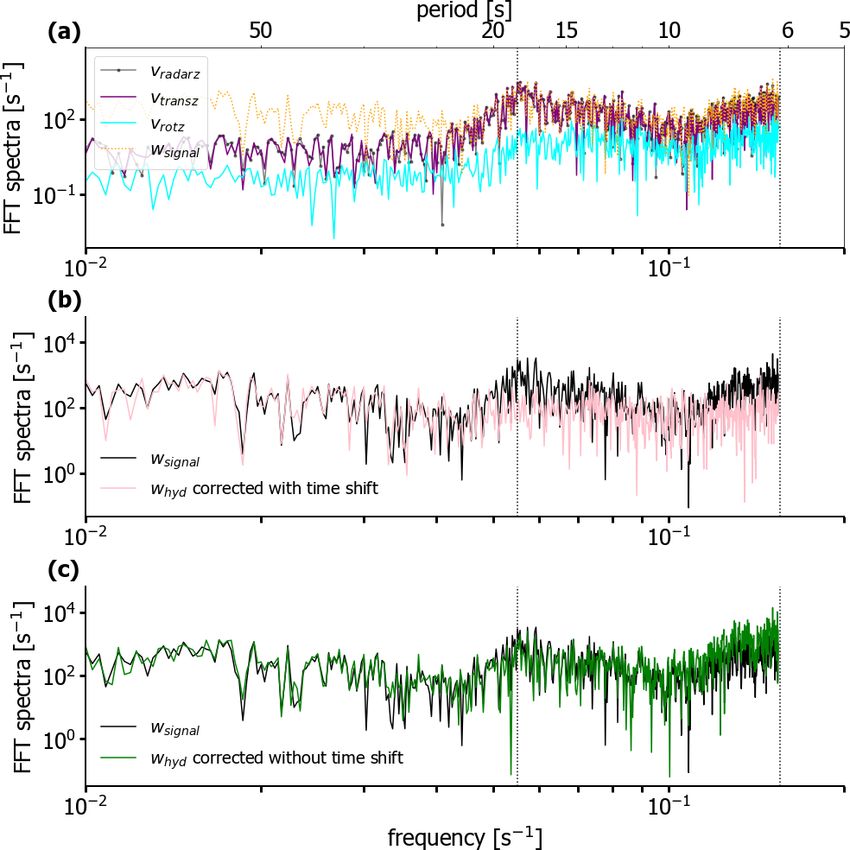
C. Acquistapace et al.: EUREC4 A’s cloud and micro rain observations from R/V Merian                                                         39

Figure 4. (a) Port and starboard with respect to the R/V MS Merian. (b) Position of the radar and its tilting due to ship motions expressed in
terms of roll, pitch, and yaw of the ship. The original position is represented by a black vector (arrow), and the position after the movement
is given by a blue arrow. The angle representing the rotation from the initial to the final position is η, the angle between the blue and the
black arrows. The roll, pitch, and yaw in which it can be decomposed are shown in blue, red, and green, respectively. The solid red and green
lines ending in filled circles of the same color represent the vector position after undergoing the rotations due first to pitch and then to yaw.
The application of the rotation with respect to roll would then bring the black array on the blue one. The sign with respect to the conventions
indicated in the text is reported in the figure.

ing and provides roll, pitch, yaw, and heave with an accuracy              that both radar datasets undergo. Synchronization of the two
of 0.03◦ , 0.03◦ , 0.075◦ , and 0.05 m, respectively (from                 is thus necessary before applying any ship motion correction.
https://www.ldf.uni-hamburg.de/en/merian/technisches/                      Section 3.2 shows how to calculate the ship motion correc-
dokumente-tech-merian/handbuch-merian-eng.pdf, last ac-                    tion term for both radar datasets, and Sect. 3.3 assesses the
cess: 23 December 2021). The MRU is mounted at the ship’s                  correction algorithm. Finally, Sect. 3.4 shows how to filter
center of gravity to clearly separate between translatory                  interference for MRR-PRO data.
and rotational movements of the ship. As the radars are
not at the ship’s center of gravity, rotational movements of               3.1   Tackling time drift between ship and radar time
the ship lead to translation of the instruments. To calculate                    stamps
these movements, it is necessary to know the position of the
instruments with respect to the MRU. They were determined                  At the beginning of the campaign, we synchronized the ship
as vectors in the ship’s coordinate system as follows (Figs. 4             and radar clock. However, the ship and radar clock cumu-
and 1c).                                                                   lated a time lag 1T that varies with time between 1 and 4 s.
                                                                           To calculate the time-varying 1T , we use the heave rate time
r W-band = [5.15; 5.40; −17.28 m]                                          series and the time series of the mean Doppler velocity aver-
r MRR-PRO = [7.18; 4.92; −17.28 m]                                         aged over the cloudy range gates < vd > of each radar pro-
                                                                           file (see Sect. 3.3 for more details on why to use the heave
   In the MRU sensor’s conventions, roll angle is positive                 rate time series). For stationary radars, i.e., radars not moving
when port goes up, pitch angle is positive when bow goes                   in time, the mean Doppler velocity (vd ) measures the mean
up, and yaw angle is positive clockwise from the heading an-               velocity of the hydrometeors in the radar volume with re-
gle. The yaw of the ship is given as the angle clockwise from              spect to the radar that results as superposition of the air mo-
north and refers to the x axis of the ship system. Finally, the            tion and the sedimentation speed of the drops. The average
coordinate for heave is negative for upward directions. The                of vd over the cloud geometrical thickness < vd > fluctuates
angle η is the angle between the initial position of the radar r           around zero in non-precipitating regions, because the sedi-
(black vector in Fig. 4) and its final position r 0 (blue vector)          mentation speed of cloud droplets is negligible, and updrafts
after a given motion due to the ship; η can be decomposed                  and downdrafts present in the cloudy column are averaged
in terms of roll θ , pitch φ, and yaw ψ (Fig. 4). The 35 % of              out. In precipitation regions instead (for example in Fig. 5 af-
the time in which the stabilization platform blocked itself in             ter 06:17:07 UTC), it becomes more and more negative, be-
a random position is represented as grey areas in Fig. 3.                  cause of a larger and persistent downdraft. When the radar
                                                                           is moving (like on the ship), < vd > additionally tracks the
3   Data processing                                                        radar motion (Fig. 5).
                                                                              By comparing the heave rate (dashed blue line) and <
This section describes the corrections applied to the data to              vd > time series (solid red line in Fig. 5), we can derive
obtain the final reference dataset. Section 3.1 describes the              the time lag 1T . Cloud droplets have a vertical speed whyd .
drift problem in time between the radar and the ship clock                 The ship moves vertically due to waves with wheave . To a

https://doi.org/10.5194/essd-14-33-2022                                                           Earth Syst. Sci. Data, 14, 33–55, 2022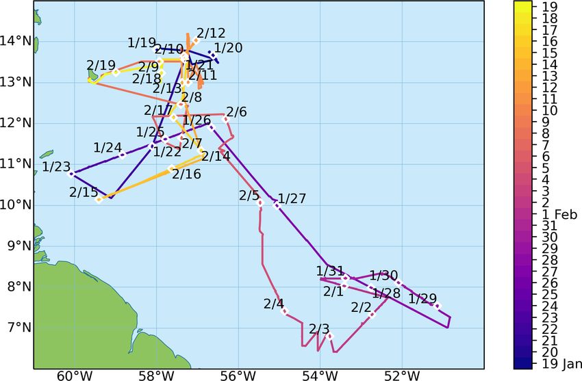
40                                      C. Acquistapace et al.: EUREC4 A’s cloud and micro rain observations from R/V Merian

Figure 5. Example of time shift application calculated to obtain the best matched correction for ship motion from the 20 January 2020 over
2 min between 6:16:17 and 6:17:57 UTC. The dashed blue line represents the vertical velocity measured by the ship wship . The dashed red
line is the mean Doppler velocity recorded by the radar at 1230 m, while the solid red line represents < vd >, the mean Doppler velocity
obtained by averaging together all cloudy pixels in each radar profile. The solid blue line represents the ship velocity after applying the time
shift of 1T = 2.65 s, and the green dots represent the values of wship finally used for correcting for ship motion. They are obtained by cubic
interpolation of the shifted ship velocity (solid blue line) on the radar time stamps. In fact, they correspond to the values of the red lines, as
expected after interpolation. In the first 7 s of the time series, a short train of three waves is clearly visible that matches the radar observed
mean Doppler velocity values much better after the time shift.

first approximation, we can neglect additional contributions               all have different time stamps. Only after matching the time
from the rotational movements of the ship (for the full vec-               series of data from the ship and data from the radar could we
torial equation see treatment in Sect. 3.2). The radar mea-                apply the ship motion correction.
sures Doppler velocity vd with respect to the instrument on
the ship; hence vd = whyd + wheave . Whereas whyd may vary                 3.2    Derivation of the ship motion’s correction formula
with height due to up- and downdrafts in the cloud, wheave is
the same within one time step for all range gates. We av-                  In the following we will derive the equations to remove ship
erage over all cloudy range gates within one time step to                  movements from the observed radar Doppler velocities with
get < vd> . By doing so we partly remove the turbulent vari-               and without a working stabilization platform. The algorithm
ation in whyd , whereas wheave remains unaffected. From the                applies to both radars. The only difference is that while for
ship’s MRU we have a time series wheave ∗    , whose time stamp            the W-band radar the correction was applied to the mean
might be shifted against the radar time series. We calculate               Doppler velocity, for the MRR-PRO the whole Doppler spec-
the variance var(1vd ) of the difference 1vd between < vd >                trum is shifted by the correction. We will adopt bold nota-
       ∗
and wheave  (dt) over a time span of 10 min for different time             tion for vectors, i.e., v = (vx , vy , vz ), where vi represents the
shifts dt. By doing so we get                                              components of the vector v along the various axes.
                              ∗
                                                                             The ship’s coordinate system is defined by a right-handed
var (1vd ) = var < vd > −wheave     · (dt) = var < whyd >                  system with unit vectors eˆx , in direction of the bow, eˆy to-

           + 2 · cov whyd , dwheave (dt) + var (dwheave (dt))              wards starboard, and eˆz perpendicular to the decks down-
                                   ∗
                                                                           wards (Fig. 4). With the ship moving in the waves, this co-
where dwheave (dt) = wheave (t) − wheave (t + dt). Ship move-              ordinate system is rotated by roll and pitch angles. This ro-
ments wheave and whyd are not correlated; i.e., the covariance             tation is described by a rotational matrix R (see Eq. C4 in
term should become zero. The equation then results in                      Appendix C). By applying the R to unit vectors of the ship

var (1vd ) = var < whyd > + var (dwheave (dt)) .           (1)             system, we get a coordinate system with eˆz pointing verti-
                                                                           cally downward in the direction of earth gravitational accel-
For an optimal time shift dt, which we call 1T , the variance              eration g and vectors eˆx and eˆy horizontally pointing in the
of the difference dwheave should become minimal (close to                  direction of the ship’s bow and starboard, respectively. We
zero), and accordingly var(1vd ) is minimal.                               call this system the horizontal coordinate system (Fig. 4).
   We then applied the resulting time lag 1T to the ship data              eˆz = [0, 0, 1] is the pointing direction of the ẑ axis of the hor-
and interpolated this shifted series to the exact radar time, ob-          izontal coordinate system and points downward.
taining the best correction term for each time stamp. We iter-                 The radar observes Doppler velocities relative to its own
ated the procedure for every radar chirp sequence since they               movement along its radar beam, and they are positive for

Earth Syst. Sci. Data, 14, 33–55, 2022                                                           https://doi.org/10.5194/essd-14-33-2022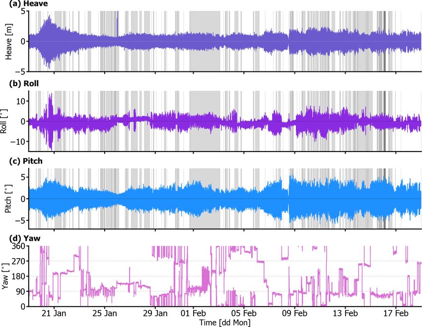
C. Acquistapace et al.: EUREC4 A’s cloud and micro rain observations from R/V Merian 41
movements away from the radar, i.e., upward for a vertical- rotation matrix R in the horizontal system, and we get
pointing instrument. The Doppler velocity measured by the êp = R∗ · eˆTp0 . The table typically got stuck at an arbi-
radar is the projection of the particle’s velocity vector on the trary position, and thus the radar points in an arbitrary
radar line of sight. Therefore, the component of the velocity direction. We reconstruct this direction by taking roll
vector of the hydrometeors wsignal measured by the radar is and pitch at time t0 just before the table got stuck and
positive when hydrometeors move upwards. The pointing di- assuming that the radar was pointing vertically at this
rection of the radar in the horizontal system is denoted as êp . moment. Orientation of the radar in the ship system
During times when the stable table is working, it is êp = −eˆz
is thus eˆTp0 = R−1 (t0 ) · (−eˆz ), which then translates to
(êp pointing upwards, eˆz pointing downwards). The velocity
observed by the radar is the relative velocity between hy- eˆp0 = [êp0 x , êp0 y , êp0 z ] = −R·R−1 (t0 )· eˆz , where R−1 is
drometeors (v hydr ) and the movement of the radar (v radar ) the inverse matrix of R (see Appendices C and D for
projected onto the pointing direction of the radar (êp ) that more details).
is The velocity vector v radar in Eq. (2) is composed of various
wsignal = v hydr − v radar · êp , (2) contributions to the motion:
where all vectors are given in the horizontal coordinate sys- v radar = v trans + v course + v rot , (7)
tem, and the dot represents the scalar product. The movement
of the hydrometeors can be decomposed in the horizontal where the velocities that add up to the radar movement are as
system into a component along the vertical axis and one in follows.
the horizontal plane:
– The translation velocity vector v trans depends on the
v hydr = vhydr,s eˆz + v wind,s , (3) translation movements of the ship: heave, surge, and
sway (we neglect the surge and sway contribution), and
where the term vhydr,s is the hydrometeor fall speed in the it is given by v trans = [0, 0, wheave ] (see Appendix E for
horizontal reference system (z component), and v wind,s is the the derivation).
horizontal wind vector in the horizontal reference system (for
the derivation, see Appendix B). Hence, we get – The course velocity vector v course is due to the travel
of the ship along its course, and it is given by v course =
wsignal = vhydr,s eˆz + v wind,s − v radar · êp . (4) [vs sin ψ, vs cos ψ, 0], where ψ is the yaw and vs is the
Now solving Eq. (4) for vhydr,s that is the hydrometeors’ fall magnitude of the ship velocity vector (see Appendix E
speed in the horizontal reference system, we get for the derivation).
– The rotation velocity vector v rot describes the move-
wsignal v wind,s − v radar · êp
vhydr,s = − . (5) ment due to the rotation of the ship (roll, pitch, yaw)
eˆz · êp eˆz · êp
and the fact that the instruments are not deployed in the
In the case of a working stabilization platform, the radar center of rotation but at distances rMRR-PRO and rW-band
pointing vector is exactly upwards, and accordingly the from it. Its expression is v rot = dR
dt · r MRR-PRO /W-band
scalar product eˆz · êp is equal to −1 as êz is pointing down- (Appendix C for the derivation of the full expression).
wards. In the limit of a non-moving ship we get vhydr,s =
−wsignal , where the opposite sign is given by the fact that 3.3 Application of the correction and additional
the ship reference system has an opposite z direction to the smoothing
one in the radar convention. Finally in the common definition
with falling hydrometeors having negative velocities, we get When the table is working and the radar is pointing vertically,
all horizontal vector components vanish, and the expression
wsignal v wind,s − v radar · êp of the corrected hydrometeor velocity reduces to
vhydr = −vhydr,s = − + . (6)
eˆz · êp eˆz · êp
w = wsignal − vtransz − vrotz , (8)
The pointing direction of the radar êp in Eq. (5) changes de-
pending on whether the stabilization platform is working or where vtransz and vrotz are the z components of the vec-
not. tors v trans and v rot . In this case, for calculating the velocity
– If the stabilization platform is working perfectly, we as- terms we need roll, pitch, and heave rate. All these data are
sume that êp = [0, 0, −1]. provided by the ship navigation system. Angles of roll and
pitch are necessary because the rotation of the ship moves the
– If the stabilization platform is not working, the pointing radar vertically. Course (yaw and speed) is not necessary as
vector of the radar moves with the ship coordinate sys- it is a horizontal component not seen by the vertical-looking
tem. Accordingly eˆp0 has to be rotated with the ship’s radar.
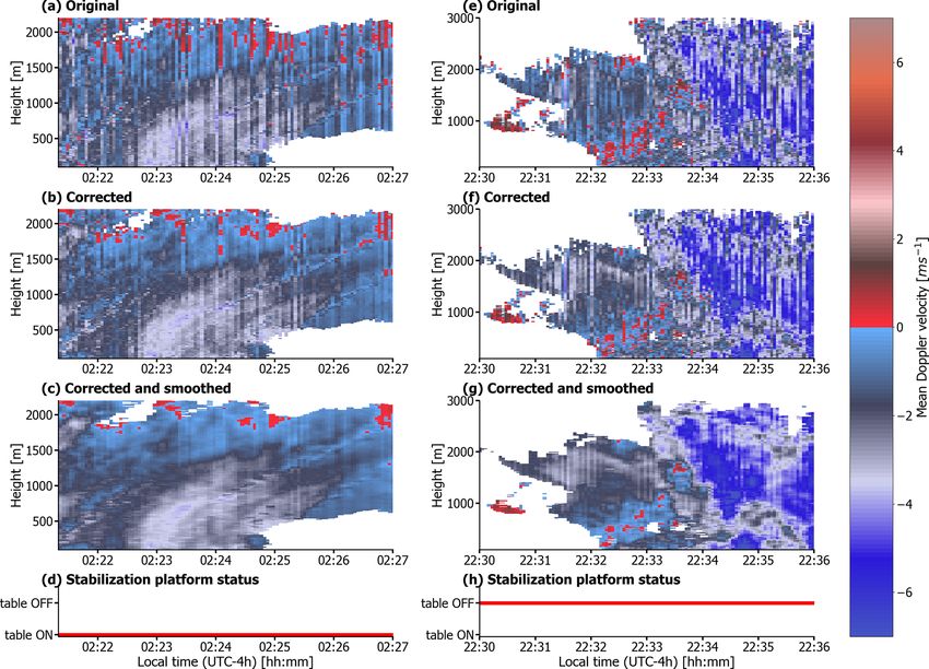
https://doi.org/10.5194/essd-14-33-2022 Earth Syst. Sci. Data, 14, 33–55, 202242 C. Acquistapace et al.: EUREC4 A’s cloud and micro rain observations from R/V Merian Figure 6. On the left is an example of the ship motion correction algorithm applied when the stabilization platform was working, on 20 January 2020 from 02:21 to 02:27 LT (UTC−4h) for the W-band radar data with de-aliasing applied: (a) original mean Doppler velocity field without any correction algorithm applied, (b) mean Doppler velocity after application of the correction from ship motions, (c) mean Doppler velocity after application of correction from ship motions and smoothing (running mean over 9 s), and (d) status of the stabilization platform. On the right is another example when the stabilization platform did not work, on 12 February 2020 between 22:30 and 22:36 LT: (e) original mean Doppler velocity field without any correction algorithm applied, (f) mean Doppler velocity after application of the correction from ship motions, (g) mean Doppler velocity after application of correction from ship motions and smoothing (running mean over 9 s), and (h) status of the stabilization platform. When the table is not working, the pointing vector of the An example of the application of the correction for ship radar is not vertical most of the time and may have a horizon- motions when the stabilization platform is working is vis- tal component (scalar products of êp with horizontal vector ible in Fig. 6a–d, for the case of 20 February 2020 be- components do not vanish). Accordingly, course of the ship tween 02:22 and 02:27 LT (local time), with especially strong and horizontal wind may contribute to the signal. We there- waves (compare with Fig. 3). fore need the additional parameters yaw and speed of the ship When comparing the original (Fig. 6a) to the corrected and the horizontal wind above. The first two are provided by mean Doppler velocity field (Fig. 6b), one can quickly no- the ship’s navigation system. For the wind we used the out- tice that many of the intense and frequent vertical bars disap- put of dedicated ICON simulations run (Daniel Klocke, per- pear, providing a more homogeneous and continuous field. sonal communication, 2020) over the EUREC4 A domain to However, the correction cannot entirely remove the distur- extract the horizontal wind profiles at the closest time and bances, as shown in Fig. 6b by some visible vertical bars re- place of the ship, corresponding to the time when the table maining despite the correction. Some possible reasons for the was not working. This type of correction affected 35 % of mismatch observed are the distance between the MRU sen- the total measurement time. The low time resolution of the sor and the radar equipment, especially considering that we model output compared to the observations made this cor- measured the radar equipment’s position by hand. We also rection less accurate than the one applied for the 65 % of the assume that the stabilization platform keeps the radar per- data in which the stabilization platform worked correctly. fectly in zenith, but it is hard to quantify the accuracy of Earth Syst. Sci. Data, 14, 33–55, 2022 https://doi.org/10.5194/essd-14-33-2022
C. Acquistapace et al.: EUREC4 A’s cloud and micro rain observations from R/V Merian                                                        43

Figure 7. (a) Fast Fourier transform (FFT) of the vertical component of vradar and of its translational (purple) and rotational (cyan) compo-
nents for 1 h of data collected at a cloudy range gate located at 1605 m from the radar (all terms along z in Eq. 7). The vradarz FFT highlights
two main wave periods around 6 and 17 s, indicated by dashed vertical lines. In the total radar velocity along z (black dotted line), the
contribution of the rotational component is minor compared to the contribution of the translational component (heave). (b) Comparison of
the FFT of the uncorrected mean Doppler velocity (black) measured by the radar and of the FFTs of the corrected mean Doppler velocity
with time shift applied. The two main wave peaks disappeared in the corrected signal (pink line). (c) Same as the middle panel, but with
the corrected mean Doppler velocity calculated without applying the time shift. In this case, the wave frequencies are not removed from the
corrected signal (green line).

such a hypothesis since a small error in the zenith alignment             22:36 LT. Even if the final smoothing (Fig. 6g) improves the
can produce disturbances. Moreover, the time lag quantifi-                vd pattern compared to the field obtained when applying the
cation 1T can be unprecise due to the reinitialization of the             correction algorithm only (Fig. 6f), overall the performance
chirp generator of the W-band radar. Such time is random and              is worse than in Fig. 6a–c, and vertical stripes are markedly
adds an unknown uncertainty to the time stamps assigned to                visible in all fields. We also applied the time shift and the ship
the measurements. Finally, the coarse temporal resolution of              motion correction to the MRR-PRO data, obtaining similar
the MRU data makes an interpolation to the radar data neces-              results as will be shown in Sect. 3.4.
sary. Figure 5 nicely shows the rapidly changing wship , which               Figure 7 for 1 h shows the impact of the time matching and
misses the real minima and maxima due to its coarse tempo-                of the correction applied to the signal in the frequency space.
ral resolution, making an interpolation challenging. We ap-               The heave rate is the main contributor to the vertical motion
plied a running mean over three time stamps (i.e., over a                 of the radar (Fig. 7a), as described by looking at a cloudy
9 s time interval) to account for these limitations (Fig. 6c).            range gate. The rotational components are approximately 1
The final signal obtained shows an almost continuous field in             order of magnitude smaller because the instruments are not
mean Doppler velocity.                                                    too far from the center of mass of the ship, and the rotation
   Figure 6e–g show the correction performance when the                   of the ship does not move the instrument much along the
table did not work, on 12 February between 22:30 and                      vertical. For this reason, it represents the vertical velocity of

https://doi.org/10.5194/essd-14-33-2022                                                          Earth Syst. Sci. Data, 14, 33–55, 2022
44                                  C. Acquistapace et al.: EUREC4 A’s cloud and micro rain observations from R/V Merian

the ship due to the waves, as previously stated. The frequen-         1. We calculated for each spectrum the prominence of all
cies of the waves at approximately 6 and 17 s (highlighted               its spectrum peaks, i.e., each peak’s ability to stand out
by the vertical dashed bars in Fig. 7) are visibly removed in            from the surrounding baseline of the signal. Then, we
the FFT spectra of the corrected mean Doppler velocity only              derived the difference between the maximum and mini-
if the time shift is applied (compare Fig. 7b and c). Finally,           mum prominence and calculated their difference (1P ).
the increase in the spectra towards the Nyquist frequency,               The difference is tiny for spectra containing only inter-
between 0.1 and 0.5 Hz, indicates that there are higher fre-             ference patterns and no signal from hydrometeors, while
quencies above 0.5 Hz, folded back into this interval. Such              it is significantly larger for a Doppler spectrum detect-
frequencies do play a role that is not resolved by MRU or by             ing hydrometeor backscattering (see for reference in
the radar itself. The final smoothing over the 9 s time win-             Fig. A1). Spectra affected by interference patterns were
dow removes the high-frequency components, and it is thus                removed by selecting spectra with 1P > 1 mm6 mm−3 ,
crucial to obtain a better signal-to-noise ratio. However, the           where the threshold value of 1 was determined empiri-
9 s smoothing degrades the average horizontal resolution of              cally.
the Vhyd,mean by a factor of 9. For an average ship speed of
3 m s−1 , the resolution would change from 3 to 27 m, result-         2. In addition, we posed a condition on the spatial con-
ing in a slightly higher resolution than the vertical 30 m one.          tinuity of mean Doppler velocity (mdv) in the lowest
However, daily maximum speeds for the ship can also reach                600 m. The mdv obtained from spectra affected by in-
9 m s−1 , thus producing a coarser resolution.                           terference shows very large random absolute values.
                                                                         Doppler spectra detecting hydrometeors produce con-
                                                                         tinuous mdv field in space. We discarded all profiles
3.4   Removal of interference patterns and correction for
                                                                         where the difference of consecutive mdv values along
      ship motions for MRR-PRO dataset
                                                                         the profile shows more than eight abrupt peaks (thresh-
The MRR-PRO electronics interfered with the ship instru-                 old decided empirically).
mentation and with the stabilization platform electronics dur-
ing the whole campaign. To be able to use the data collected,         3. We apply a spatial filtering to remove spurious noisy
we removed the interference patterns using a noise removal               pixels: the filters exclude all pixels where 1P > 1 that
mask. The interference draws periodical disturbances with                have fewer than three adjacent neighbors fulfilling the
peak intensity decreasing with height. Since the interference            same condition.
peaks are larger than the mean noise level calculated using
                                                                  It is almost impossible to distinguish the signal due to hy-
the Hildebrand–Sekhon method by the manufacturer’s pro-
                                                                  drometeors from the one due to interference in the reflectivity
cessing (Hildebrand and Sekhon, 1974), multiple small peaks
                                                                  field Ze of the original dataset. However, after applying the
appear in the MRR-PRO spectra. The mean Doppler veloc-
                                                                  noise removal mask the hydrometeor signal becomes clearly
ity and the spectral width of such noise spectra are random,
                                                                  visible (Fig. 8a and b). The time correction (see Sect. 3.1)
depending on which noise peak is the highest (Fig. A1).
                                                                  and post-processing tool from Garcia-Benadí et al. (2021)
   The MRR-PRO dataset produced by the software of the
                                                                  were then applied to remove the time lag 1T and de-alias
manufacturer is initially processed with the MRR-PRO post-
                                                                  and obtain a physically realistic Doppler velocity range for
processing tool (Garcia-Benadí et al., 2021). The algorithm
                                                                  all Doppler spectra above the noise level (Anti-aliasing in
allows us to obtain de-aliased Doppler spectra over a physi-
                                                                  Fig. 8). Then, ship motion correction derived with the calcu-
cally realistic Doppler velocity range. For data with 5 or 10 s
                                                                  lations presented in section 3.2 is applied and all the main
integration time, this tool is sufficient to remove the inter-
                                                                  MRR-PRO variables of interest are derived from the cor-
ference pattern. No ship motion correction can be applied
                                                                  rected Doppler spectra. Figure 8d shows a hook rain struc-
to those data because their integration time is larger than or
                                                                  ture visible, possibly caused by downdraft wind mixing. The
similar to the typical wave period (see Fig. 7a), and Doppler
                                                                  vortex structure was not visible in the original data (Fig. 8c)
variations due to heave motions are smoothed out. We resam-
                                                                  and emerged from the noise after applying the correction on
pled the data collected from 19 to 25 January 2020 with 5 s
                                                                  the mean Doppler velocity field.
to 10 s integration time, to reduce the impact of ship motions
completely.
   The post-processing of the data collected with 1 s integra-    4    Characteristics of trade wind cumulus clouds and
tion time, i.e., from 25 January to 19 February 2020, is more          precipitation
complex. For the 1 s resolution data, the tool from Garcia-
Benadí et al. (2021) cannot remove the interference patterns      To give an overview of the meteorological conditions en-
as it did for the 10 s integration time dataset. Hence, to ob-    countered on each of the 32 d of campaign, Table 3 lists the
tain Doppler spectra without interference, we applied a noise     daily mean atmospheric temperature (T2m), rain rate (RR),
removal mask (interference filter in Fig. 8) based on specific    liquid water path (LWP), relative humidity (RH), and pres-
conditions.                                                       sure (P ) for each day of the campaign. They are collected at

Earth Syst. Sci. Data, 14, 33–55, 2022                                                 https://doi.org/10.5194/essd-14-33-2022
C. Acquistapace et al.: EUREC4 A’s cloud and micro rain observations from R/V Merian 45 Figure 8. (a) MRR-PRO attenuated reflectivity on 13 February 2020 at 01:00 UTC after manufacturer processing, without any additional interference filtering or ship motion correction. (b) Same as (a), but with the noise removal mask applied. (c) MRR-PRO mean Doppler velocity without any correction over a 2 min time interval selected from the time interval shown in (a) between 01:32 and 01:35 UTC and (b) and highlighted with dashed black lines. Vertical stripe structures are visible due to ship motions. (d) Same as (c) but with interference removed and time shift and ship motion corrections applied to the data. The striped structure present in (c) almost entirely disappeared. the radar base, which is approximately 20 m a.s.l. (above sea level). Figure 9 shows that the vast majority of the encountered liquid clouds have a LWP smaller than 100 g m−2 , with a median value of 11 g m−2 in agreement with Schnitt et al. (2017), who sampled the region between 10 and 20◦ N and −40 and −60◦ W in December 2013. Noise and gain drifts in the passive channel of the radar lead to positive LWP re- trieved values even in clear-sky conditions. These data have a median and standard deviation of 1.2 and 5.4 g m−2 , re- spectively, which are within the retrieval uncertainty (about 30 g m−2 ). The standard deviation of the clear-sky distribu- tion can be considered a sort of uncertainty of the LWP val- ues retrieved with the neural network algorithm and can be used to correct the LWP values, as done in Jacob et al. (2019). We compared the obtained IWV values with the IWV re- Figure 9. LWP distribution for cloudy (blue) and clear-sky (red) trieved from GNSS by Bosser et al. (2021). The mean of the conditions, for the whole campaign. IWV retrieved from W-band radar single-channel retrieval is 31.7 kg m−2 , the median is 32.3 kg m−2 , and the standard de- viation of the distribution is 5.15 kg m−2 . The bias between the GNSS IWV estimations from MS Merian (Bosser et al., the mean value of the IWV distribution from W-band and the 2021), as well as to limitations in the IWV single-channel IWV distribution from GNSS is 3.4 kg m−2 , which is con- retrieval. sistent with the bias estimated with ground-based GNSS sta- To show the full potential of the collected radar dataset, tions reported in Fig. 9 of Bosser et al. (2021). The spread we display one case study of an extended precipitating between the GNSS and the radar-derived values of IWV can cloud field occurring on 12 February 2020 from 15:00 to be due to the strongly varying bias component that affects 17:00 UTC in the trade wind alley at about 13.5◦ N and https://doi.org/10.5194/essd-14-33-2022 Earth Syst. Sci. Data, 14, 33–55, 2022
46                                    C. Acquistapace et al.: EUREC4 A’s cloud and micro rain observations from R/V Merian

Table 3. Daily mean values of the main surface variables observed     radar system collected echoes in the first 2200 m, showing
on the MS Merian during the EUREC4 A campaign: T2m is the             the complex internal structure of the clouds. The cloud base
air temperature 2 m above the radar base, which is approximately      detected from the W-band radar ranges between 750 and
20 m a.s.l. (above sea level), RR is the rain rate. The liquid wa-    1250 m and does not exactly correspond with the lifting con-
ter path (LWP) is derived from the collocated 89 GHz channel mi-      densation level (LCL) values (black solid line in Fig. 10a
crowave radiometer, and RH and P are the relative humidity and air
                                                                      and b) obtained for this case, while in non-precipitating con-
pressure from a weather station positioned next to the radar equip-
ment.
                                                                      ditions LCL is higher. Cloud top ranged between 1700 and
                                                                      2100 m.
 Day             T2m           RR         LWP     RH        P            The high-vertical-resolution mode for the W-band radar
                 [◦ C]    [mm h−1 ]    [g m−2 ]   [%]     [hPa]       (7 m up to 1230 and 9 m from 1230 to 3000 m) detected
                                                                      distinctive features in the radar moments (Fig. 11a–d). Fil-
 19 Jan 2020     26.35          0.0          1    63.6   1013.9
                                                                      aments of higher reflectivity between 15:53 and 15:55 UTC
 20 Jan 2020     25.95         0.57         30    72.4   1013.3
 21 Jan 2020     26.85          1.0         71    67.2   1011.7       at around 800 m (Fig. 11a) suggest a correlation of the size
 22 Jan 2020     27.25         1.42          0    63.2   1010.3       of the drops with air motions; Fig. 11b displays clear areas
 23 Jan 2020     26.85         0.99         12    69.2   1009.7       in the cloud where larger mean Doppler velocities are asso-
 24 Jan 2020     26.15         0.57        318    76.2   1010.4       ciated with heavy rain. The spectral width field (Fig. 11c)
 25 Jan 2020     26.85         0.67         13    67.5   1011.9       also benefits from the high temporal and spatial resolution.
 26 Jan 2020     26.65          0.0         23    67.4   1012.2       It shows patterns that suggest a correlation between large
 27 Jan 2020     26.95         1.37        391    75.2   1012.0       reflectivities and mean Doppler velocity values as well as
 28 Jan 2020     27.25          0.0         50    74.9   1010.8       large spectral width values. Finally, the skewness field shows
 29 Jan 2020     27.15         0.32         26    72.4   1010.9
                                                                      patches of positive and negative skewness emerging from the
 30 Jan 2020     27.55          0.0         20    71.5   1011.7
 31 Jan 2020     27.35          0.0          8    70.0   1012.7       noise. Further analysis of the Doppler spectra in precipitation
 1 Feb 2020      27.45         0.31         13    64.8   1013.0       is necessary to interpret these patches and exploit the skew-
 2 Feb 2020      27.45         0.49          6    62.3   1012.0       ness signatures (Acquistapace et al., 2019).
 3 Feb 2020      27.05          0.0          3    68.2   1013.3          Also, for the MRR-PRO, the high vertical and time res-
 4 Feb 2020      27.25          0.0          8    69.2   1013.1       olution allowed us to reveal relevant structures in the lower
 5 Feb 2020      27.05         0.45         10    68.3   1014.1       precipitation field. Despite the small gaps caused by the fil-
 6 Feb 2020      27.15          0.0         11    65.7   1013.9       tering of the interference, the reflectivity (Fig. 11e) shows a
 7 Feb 2020      26.75         1.77         31    63.7   1013.9       decrease in the Ze values with decreasing altitude possibly
 8 Feb 2020      26.55         7.43         35    65.8   1013.6
                                                                      due to evaporation and/or shear. The case study highlights
 9 Feb 2020      26.85         1.38          4    66.3   1015.3
 10 Feb 2020     26.65         0.80        106    67.3   1015.1       a large variability of fall speeds in the lowest 300 m, possi-
 11 Feb 2020     26.55         0.30         54    68.7   1014.6       bly connected with sub-cloud layer dynamics. The fall speed
 12 Feb 2020     26.35         0.43         85    70.3   1014.1       field can also trace such dynamics, like the vortex structure
 13 Feb 2020     26.55         0.70         51    68.5   1012.7       in Fig. 8d. Also, the rainfall rate shows a substantial decrease
 14 Feb 2020     27.35         3.24         53    67.3   1012.9       as rain approaches the ground during the selected case study
 15 Feb 2020     26.85         0.89         22    68.0   1012.1       (Fig. 11g). During the case study the stabilization platform
 16 Feb 2020     26.75         1.06         47    70.2   1011.3       worked continuously and the LWP registered high values and
 17 Feb 2020     27.05         0.33         15    68.6   1011.9
                                                                      saturated (LWP > 1000 g m−2 ) under rainy conditions. Note
 18 Feb 2020     26.75         4.22        312    71.4   1013.2
                                                                      that values above 1000 g m−2 should not be considered reli-
 19 Feb 2020     26.05         0.62        319    74.1   1013.1
                                                                      able because of contamination due to rain.

                                                                      5    Data availability
57◦ W. On that date, the ship encountered a cloud system
identifiable as a flower type (Bony et al., 2020) using the cor-      The data presented in this paper can be accessed at the
rected reflectances from Moderate Resolution Imaging Spec-            AERIS repository and in the ARM database in NetCDF for-
troradiometer (MODIS) TERRA (Platnick et al., 2003), with             mat, under https://doi.org/10.25326/235 (Acquistapace et al.,
a diameter between 200 and 250 km that generated precipita-           2021c). This DOI was assigned to the new version of the
tion during the afternoon (Fig. 10c). When comparing the              dataset, produced after fixing a bug in the standard post-
signals observed by the W-band radar (Fig. 10a) and the               processing script and correcting the LWP neural network
MRR-PRO (Fig. 10b), the different sensitivities of the two            dataset. In the dataset the following applies.
instruments become evident: while the W-band is capable of
detecting cloud and precipitating hydrometeors, the MRR-                  – Technical radar variables were removed and stored in
PRO is sensitive to larger raindrops only. The interference                 hourly technical files that can be accessed upon email
patterns reduced the ability of the MRR-PRO to detect pre-                  request to the paper’s corresponding author.
cipitation in a way that it is difficult to quantify. The W-band

Earth Syst. Sci. Data, 14, 33–55, 2022                                                   https://doi.org/10.5194/essd-14-33-2022
You can also read