An aerosol classification scheme for global simulations using the K-means machine learning method
←
→
Page content transcription
If your browser does not render page correctly, please read the page content below
Geosci. Model Dev., 15, 509–533, 2022
https://doi.org/10.5194/gmd-15-509-2022
© Author(s) 2022. This work is distributed under
the Creative Commons Attribution 4.0 License.

An aerosol classification scheme for global simulations using the
K-means machine learning method
Jingmin Li, Johannes Hendricks, Mattia Righi, and Christof G. Beer
Deutsches Zentrum für Luft- und Raumfahrt (DLR), Institut für Physik der Atmosphäre, Oberpfaffenhofen, Germany

Correspondence: Jingmin Li (jingmin.li@dlr.de)

Received: 8 June 2021 – Discussion started: 23 July 2021
Revised: 2 November 2021 – Accepted: 15 December 2021 – Published: 25 January 2022

Abstract. The K-means machine learning algorithm is ap-            for aerosol research. To estimate the uncertainties inherent in
plied to climatological data of seven aerosol properties from      the applied clustering method, two sensitivity tests have been
a global aerosol simulation using EMAC-MADE3. The aim              conducted (i) to investigate how various data scaling proce-
is to partition the aerosol properties across the global atmo-     dures could affect the K-means classification and (ii) to com-
sphere in specific aerosol regimes; this is done mainly for        pare K-means with another unsupervised classification algo-
evaluation purposes. K-means is an unsupervised machine            rithm (HAC, i.e. hierarchical agglomerative clustering). The
learning method with the advantage that an a priori definition     results show that the standardization based on sample mean
of the aerosol classes is not required. Using K-means, we are      and standard deviation is the most appropriate standardiza-
able to quantitatively define global aerosol regimes, so-called    tion method for this study, as it keeps the underlying distri-
aerosol clusters, and explain their internal properties and        bution of the raw data set and retains the information of out-
their location and extension. This analysis shows that aerosol     liers. The two clustering algorithms provide similar classifi-
regimes in the lower troposphere are strongly influenced           cation results, supporting the robustness of our conclusions.
by emissions. Key drivers of the clusters’ internal proper-        The classification procedures presented in this study have a
ties and spatial distribution are, for instance, pollutants from   markedly wide application potential for future model-based
biomass burning and biogenic sources, mineral dust, anthro-        aerosol studies.
pogenic pollution, and corresponding mixtures. Several con-
tinental clusters propagate into oceanic regions as a result
of long-range transport of air masses. The identified oceanic
regimes show a higher degree of pollution in the Northern          1   Introduction
Hemisphere than over the southern oceans. With increas-
ing altitude, the aerosol regimes propagate from emission-         Aerosols play an important role in the climate system
induced clusters in the lower troposphere to roughly zon-          (Boucher et al., 2013). They influence climate directly via
ally distributed regimes in the middle troposphere and in the      scattering and absorption of solar and terrestrial radiation
tropopause region. Notably, three polluted clusters identified     and indirectly via modifications of cloud properties. The ma-
over Africa, India, and eastern China cover the whole atmo-        jor components of atmospheric aerosols are mineral dust,
spheric column from the lower troposphere to the tropopause        black carbon (BC), organic carbon, sulfate, nitrate, ammo-
region. The results of this analysis need to be interpreted tak-   nium, and sea salt. Due to their relatively short residence
ing the limitations and strengths of global aerosol models         times, the contributions of these components, their state of
into consideration. On the one hand, global aerosol simula-        mixing, and the particle size distribution show a large spa-
tions cannot estimate small-scale and localized processes due      tial and temporal variability on the global scale (e.g. Lauer
to the coarse resolution. On the other hand, they capture the      and Hendricks, 2006; Mann et al., 2010, 2014; Pringle et
spatial pattern of aerosol properties on the global scale, im-     al., 2010; Aquila et al., 2011; Sessions et al., 2015; Kaiser
plying that the clustering results could provide useful insights   et al., 2019). Additionally, their effects on clouds and radia-
                                                                   tion are highly variable due to the strong dependencies on

Published by Copernicus Publications on behalf of the European Geosciences Union.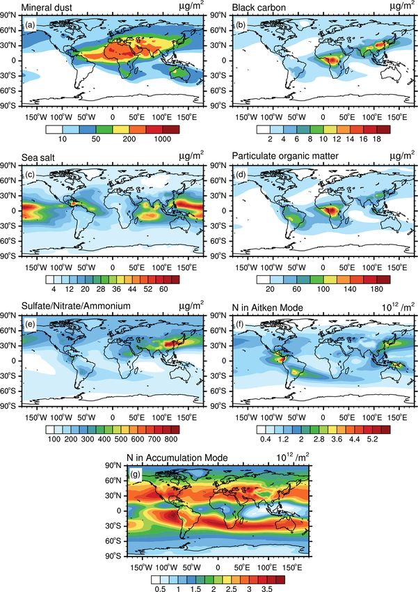
510                                                          J. Li et al.: An aerosol classification scheme for global simulations

the physical and chemical properties of the aerosols. This            der these circumstances, analysing all relevant variables from
in combination with uncertainties in the current knowledge            a typical global model simulation can become unfeasible.
of key aerosol-related processes makes the quantification of          New analysis methods are therefore required to gather in-
aerosol–climate effects a challenge and results in compara-           formation from the huge set of variables and their tempo-
tively large uncertainties in the existing quantifications of the     ral and spatial variability. A powerful tool to facilitate the
climate impact of anthropogenic aerosols (e.g. Boucher et al.,        analysis of global aerosol model results is the partitioning
2013; Myhre et al., 2017; Bellouin et al., 2020).                     of the model-simulated aerosol into different groups or clus-
   Global aerosol–climate models equipped with detailed               ters, each characterized by specific properties. In the follow-
representations of aerosol microphysical and chemical pro-            ing, these groups will be called aerosol regimes. Informa-
cesses are essential tools for the quantification of aerosol–         tion about how these aerosol regimes are distributed in space
climate effects (e.g. Boucher et al., 1998; Takemura et al.,          could be very helpful to obtain a concise but comprehensive
2005; Stier et al., 2005, 2006; Lauer et al., 2007; Hoose et al.,     view of the complex system of modelled aerosol parameters.
2008; Righi et al., 2013, 2020; Randles et al., 2013; Kipling         Detailed knowledge of the spatial distribution of individual
et al., 2016; Myhre et al., 2017; Bellouin et al., 2020). Dur-        aerosol regimes could be the basis for further analyses and
ing the last few decades, considerable attempts have been             model improvement. For instance, observations within a spe-
made by the global aerosol modelling community to develop             cific aerosol regime can be combined for evaluating simula-
improved descriptions of aerosol–climate interactions (e.g.           tion results with regard to this specific aerosol type. Further-
Ghan and Schwartz, 2007; Boucher et al., 2013; Riemer et              more, model evaluation results based on observations lim-
al., 2019). Early modelling approaches considered only the            ited in space and time (e.g. aircraft-based field campaigns),
mass of aerosol species. However, observations imply that             could be generalized to a whole aerosol regime covering
the number, size distribution, and mixing state of aerosols are       much larger areas and time periods, assuming that the sys-
also critical factors for an accurate representation of aerosol–      tematic model biases to be corrected occur nearly homoge-
climate interactions (Albrecht et al., 1989). The first attempts      nously throughout the whole cluster. In addition, knowledge
at representing the aerosol size distribution and mixing state        of the properties and spatial extension of aerosol regimes
in global models started at the end of the 20th century (e.g.         could serve as supportive information for satellite retrieval
Jacobson, 2001). Due to limited computing capacities and the          and for the planning of further field campaigns for aerosol
huge computational expenses of global aerosol–climate mod-            observation.
els, cost-effective algorithms have been applied, for instance,          Previous aerosol classifications have been mainly con-
the lognormal representations of the aerosol size distribution        ducted in the context of observational studies using mea-
(e.g. Stier et al., 2005; Lauer et al., 2006; Aquila et al., 2011;    surements of aerosol microphysical and optical properties.
von Salzen, 2006; Pringle et al., 2010; Kaiser et al., 2019).         For example, Groß et al. (2013, 2015) applied classification
Recent approaches allow for tracking soluble and insoluble            schemes to identify specific aerosol types and their mixtures
aerosol particle components, as well as their mixtures, and           based on lidar measurements and satellite data. Their clas-
facilitate the simulation of particle number, mass concentra-         sification procedure follows a tree structure where different
tion, and size distribution. Beyond the direct radiative im-          aerosol microphysical and optical properties imply differ-
pact of aerosols, aerosol–cloud interactions are key processes        ent classification branches. This allows the identification of
driving aerosol–climate effects. Hence, parameterizations of          complicated vertical stratifications of different aerosol types
aerosol activation in liquid clouds have been established (see        throughout the atmosphere. Bibi et al. (2016) applied multi-
Ghan et al., 2011, for a review). In addition, aerosol-induced        ple clustering techniques to analyse seasonal differences in
formation of ice crystals has attracted increasing attention          prevailing aerosol types at four locations in India. Their clas-
(Kanji et al., 2017; Heymsfield et al., 2017). To represent the       sification was based on the analysis of pairs of aerosol op-
manifold ice formation pathways induced by a large num-               tical properties gained from the Aerosol Robotic Network
ber of different aerosol types in global aerosol–climate mod-         (AERONET) sun photometer measurements. Schmeisser et
els, the applied microphysical cloud schemes, as well as the          al. (2017) applied a similar multiple clustering technique to
underlying aerosol sub-models, have been further extended             classify aerosol types based on surface-based observations
(e.g. Lohmann and Kärcher, 2002; Kärcher et al., 2006;                of spectral aerosol optical properties from a global station
Lohmann et al., 2007; Lohmann and Hoose, 2009; Hendricks              network. Nicolae et al. (2018) classified six aerosol types
et al., 2011; Kuebbeler et al., 2014; Righi et al., 2020).            using an artificial neural network applied to lidar measure-
   The above examples demonstrate the growing complex-                ments. The neural network was trained with predefined data
ity of global aerosol models, which consequently results in a         from different aerosol types. Applying similar algorithms to
large number of parameters that describe the aerosol number           global model results using optical aerosol properties to clas-
concentration, size distribution, and composition and makes           sify aerosol types, however, could be problematic since the
the analysis, evaluation, and interpretation of the model re-         optical properties are derived quantities that are calculated
sults a challenge. This is further complicated by the large           from primary (prognostic) quantities such as aerosol number,
spatial and temporal variability of the aerosol properties. Un-       size, and composition. These calculations also require addi-

Geosci. Model Dev., 15, 509–533, 2022                                                   https://doi.org/10.5194/gmd-15-509-2022
J. Li et al.: An aerosol classification scheme for global simulations                                                           511

tional assumptions, usually retrieved from measurements of,         of the global clustering procedure are presented in Sect. 3,
e.g. aerosol refractive indices, possibly implying further un-      including separate discussions of the three predefined atmo-
certainties (Dietmüller et al., 2016). Hence, new algorithms        spheric layers. Section 4 provides an uncertainty analysis by
for aerosol classification based on primary aerosol model pa-       testing various sensitivities of the obtained results to method-
rameters would be more appropriate.                                 ical aspects in view of the limitation and strength of global
   In this study, we apply the K-means machine learning clus-       aerosol models and potential applications of the presented
tering algorithm (Hartigan and Wong, 1979) for identifying          clustering method. A summary of the main conclusions and
clusters of specific aerosol types in global aerosol simula-        an outlook are given in Sect. 5.
tions. This method partitions n samples into k clusters in
which each sample is assigned to the cluster with the nearest
distance to the clusters’ centre (or cluster centroid). K-means     2     Data and methods
is classified as an unsupervised machine learning algorithm.
This is especially useful when the classification criteria are      2.1    Model description and configuration
unknown, as in the case of aerosol classification where the
specific aerosol characteristics for the predominant regimes        As a basis for aerosol classification in the present study,
are not known a priori. In comparison with supervised clas-         we analyse one of the global model simulations of Beer et
sification algorithms, which require substantial prior knowl-       al. (2020) performed with the global aerosol model EMAC-
edge of classes, an unsupervised classification is relatively       MADE3. MADE3 simulates nine different aerosol species
easy to use, but it requires the identification and labelling       (sulfate, ammonium, nitrate, the sea salt species sodium and
of the resulting clusters after the classification. The common      chloride, BC, POM, mineral dust, and aerosol water). These
known limitations of K-means include the presence of clus-          nine aerosol species occur in three different internal mix-
ters with equal variances and its sensitivity to outliers. K-       tures (purely soluble particles, mixed particles consisting of
means has already been applied in atmospheric research. For         an insoluble core with a soluble coating, and particles mainly
instance, it has been successfully used to distinguish clouds       composed of insoluble material and only very thin soluble
and aerosols in CALIOP/CALIPSO observations (Zeng et                coatings) within three size modes (Aitken, accumulation, and
al., 2019). In this study, we apply the K-means algorithm to        coarse mode). This results in a total of nine aerosol modes.
global aerosol simulations. The main goal is to answer the          The model considers particle transformations due to coagu-
following questions: (1) how can major aerosol regimes be           lation, condensation, gas–particle partitioning, and new par-
identified in global aerosol simulations, (2) what is the spatial   ticle formation. MADE3 was evaluated in detail in past stud-
distribution of these regimes, and (3) which aerosol types are      ies and showed a generally good model performance. Kaiser
dominant in which parts of the world? The K-means method            et al. (2014) demonstrated the ability of MADE3 to repre-
is applied here to identify clusters of different aerosol types     sent the aerosol microphysical processes when compared to
in global simulations. The spatial extension of these clusters      a more detailed particle-resolving aerosol model. Kaiser et al.
is quantified. The aerosol properties considered for the clus-      (2019) further demonstrated a good agreement of BC, POM,
tering process were simulated using the global chemistry–           gaseous species, and particle number concentrations simu-
climate model system EMAC (the ECHAM/MESSy Atmo-                    lated with EMAC-MADE3 with various observations. Beer
spheric Chemistry general circulation model, Jöckel et al.,         et al. (2020) further extended the model set-up of Kaiser
2010, 2016) equipped with the aerosol microphysical sub-            et al. (2019) by including an online parameterization for
model MADE3 (Modal Aerosol Dynamics model for Europe                wind-driven dust emissions (Tegen et al., 2002) and per-
adapted for global applications, third generation, Kaiser et        formed five model experiments for the time period 2000–
al., 2014, 2019). The aerosol properties analysed here include      2013 in different horizontal and vertical model resolutions.
the mass concentrations of mineral dust; BC; particulate or-        The model results were evaluated by comparison against ob-
ganic matter (POM); sea salt; the sum of aerosol sulfate, ni-       servational data from the AERONET station network (Hol-
trate, and ammonium (SNA); and particle number concentra-           ben et al., 1998, 2001) and aircraft-based measurements from
tions in different aerosol size modes. The clustering analysis      the SALTRACE field campaign (Weinzierl et al., 2017). The
is conducted separately for the lower troposphere, the middle       comparison in Beer et al. (2020) showed that a specific con-
troposphere, and the tropopause region. To quantify poten-          figuration (T63L31Tegen) outperforms the others thanks to
tial uncertainties of the clustering procedure, the sensitivity     its higher resolution and the more detailed representation of
of the results to different methods for scaling the input data      dust emission processes. Hence, data from this simulation are
is explored. We also provide a comparison of K-means clus-          used for the clustering analysis in the present study.
tering with another unsupervised machine learning cluster-             For the chosen simulation Beer et al. (2020) applied
ing algorithm, namely hierarchical agglomerative clustering         EMAC in nudged mode, meaning that model dynamics were
(HAC).                                                              constrained using ECMWF reanalysis data (Dee et al., 2011)
   The paper is structured as follows. Section 2 describes the      including wind divergence and vorticity, temperature, and the
model data and the analysis methods in detail. The results          logarithm of the surface pressure for the years 2000 to 2013.

https://doi.org/10.5194/gmd-15-509-2022                                                  Geosci. Model Dev., 15, 509–533, 2022
512                                                        J. Li et al.: An aerosol classification scheme for global simulations

Transient emission data for anthropogenic sources were used         6 for the tropopause region (∼ 300 to ∼ 100 hPa). Note that
to match this simulation period. Anthropogenic emissions            EMAC vertical levels are ordered from top to bottom. Due
were chosen according to the ACCMIP (Atmospheric Chem-              to the terrain-following hybrid sigma pressure level concept,
istry and Climate Model Intercomparison Project; Lamarque           these layers only approximately correspond to specific pres-
et al., 2010) inventory with RCP 8.5 scenario (Riahi et al.,        sure levels. Deviations can occur over elevated terrain (e.g.
2007, 2011). Biomass burning emissions were taken from              the Tibetan Plateau) in particular, as the pressure is lower in
the Global Fire Emission Database version 4 (GFED; van der          the layer than in other areas. This layer definition in the sta-
Werf et al., 2017). The wind-driven emissions of mineral dust       tistical analysis, however, is more flexible and can easily be
and sea salt were calculated online for every model time step       adopted to the respective applications.
following the dust parameterization developed by Tegen et
al. (2002) and the parameterization of sea spray introduced         2.3   Method
by Guelle et al. (2001), respectively. As mentioned above,
the model was applied at a T63L31 resolution, corresponding         The K-means algorithm used in this study is an unsuper-
to a 1.9◦ × 1.9◦ horizontal resolution and 31 vertical hybrid       vised machine learning algorithm that does not require train-
pressure levels covering the vertical range from the surface        ing data based on known and established classifications. It
up to 10 hPa. For a more detailed description of the simula-        was first introduced by MacQueen (1967), and a more ef-
tion set-up, we refer to Beer et al. (2020). Some important         ficient version of K-means was developed by Hartigan and
aspects regarding the quality of the aerosol representation in      Wong (1979). K-means is a procedure based on the calcula-
this simulation, as well as the advantages and disadvantages        tion of the squared Euclidean distance (Spencer, 2013). The
of global aerosol models in general, are further discussed in       Euclidean distance describes the distance between two points
Sect. 4.3.                                                          in the Euclidean space that can be spanned in any integer
                                                                    dimensions. Assuming that p and q are two points in a j -
2.2   Data                                                          dimensional space, the Euclidean distance d(p, q) between
                                                                    p and q is calculated by
Seven aerosol parameters extracted from the Beer et al.                         q
(2020) simulation are considered for the clustering process:        d(p, q) =       (p1 − q1 )2 + (p2 − q2 )2 + . . . + (pj − qj )2 .
the mass concentrations of mineral dust; BC; POM; sea salt;                                                                             (1)
the sum of the sulfate, nitrate, and ammonium concentration
(SNA); and Aitken and accumulation mode particle number             The K-means method partitions a sample set into a prede-
concentration Nakn and Nacc of the combined aerosol species.        fined number of clusters (k) using minimization within clus-
Using number properties in addition to mass properties is           ter variances. The basic input of the algorithm is a sam-
helpful since the number ratio of small to large particles can      ple X = {x 1 , . . ., x n } with x m = (x1m , x2m , . . .xjm ) and m ∈
change even when the total mass stays constant. The number          {1, . . ., n}, where n is the number of data points and j is the
concentrations of coarse-mode particles are not taken into          number of variable properties. The sample X is grouped into
account to avoid the duplication of information, since they         k cluster subsets (S1 , S2 , . . .Sk ) by minimizing the sum of the
are strongly correlated with the mass concentration of sea          variances within each cluster Si=1,...,k as follows:
salt and mineral dust, owing to a comparatively small vari-
                                                                             k
ability in the size distributions of the modelled mineral dust       arg min X X
                                                                                 kx − µi k2 ,                                           (2)
and sea salt particles. Since the size distributions of the mod-        S
                                                                                i=1 X∈Si
elled Aitken and accumulation modes are more variable, the
number concentrations of these particles are considered in          where µi is the centre of cluster Si (also called cluster cen-
addition to the corresponding mass concentrations. The clus-        troid) and the term kx −µi k is a simplified notation of Eq. (1)
tering process is intended to identify model grid points with       describing the Euclidean distances between all samples in x
similar climatological mean aerosol parameters as a basis to        and their cluster centre µki=1 in j Euclidean dimensions. The
classify the global aerosol distribution in different aerosol       argmin operator identifies the set of clusters Si=1,...,k , which
regimes.                                                            minimizes the total sum of the Euclidean distance. By apply-
   The simulation data from years 2000 to 2013 are first re-        ing this procedure, each member of X is assigned to a specific
duced to multi-year (14-year) means to investigate the dis-         cluster. K-means is a stepwise forward iteration process. In
tribution of climatological aerosol regimes. To account for         the first step, the cluster centroids are assigned randomly and
the vertical variability of aerosol properties, the model data      a prototype of the clusters is first estimated using Eq. (2).
at 31 vertical levels in the terrain-following hybrid sigma         Following this, in the second step, the cluster centroids are
pressure level are used to calculate values for three atmo-         replaced by prototype cluster means. These two steps are it-
spheric layers. More specifically, we integrate model level         erated until the cluster centroids change only marginally or
L31-22 for the lower troposphere (up to ∼ 700 hPa), L21-14          even stay constant. At this point the corresponding clusters
for the middle troposphere (∼ 700 to ∼ 300 hPa), and L13-           can be regarded as the optimal set of clusters.

Geosci. Model Dev., 15, 509–533, 2022                                                    https://doi.org/10.5194/gmd-15-509-2022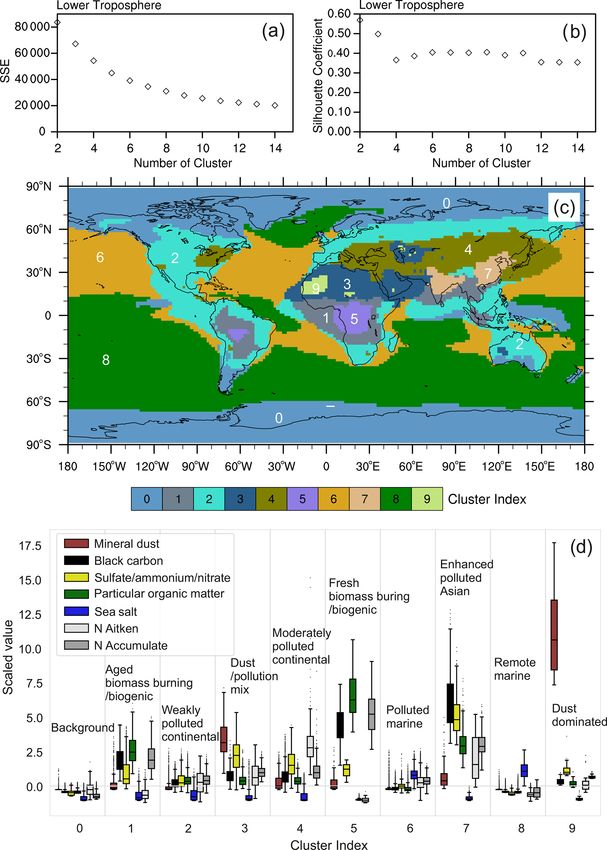
J. Li et al.: An aerosol classification scheme for global simulations                                                               513

   Selecting the number of clusters k is one of the most                tive standard deviation (StandardScaler method in the scikit-
challenging tasks in cluster analysis. Researchers developed            learn package):
many different approaches to select k, but there is no standard
solution which can be generally applied (e.g. Rousseeuw,                        xl − xl
                                                                        xls =           ,                                           (6)
1987; Sugar and James, 2011; Amorim and Hennig, 2015).                             σl
In this study we use clustering evaluation metrics in com-
                                                                        where xls stands for standardized data, xl is the original data,
bination with a plausibility check for evaluation of the ob-
                                                                        xl is the mean, and σl is the standard deviation of this spe-
tained clusters. Two clustering evaluation metrics commonly
                                                                        cific aerosol property l calculated from the whole set of
used are the sum of squared errors (SSE) and the silhouette
                                                                        samples. The standardization ensures the comparability of
coefficient (SC; Rousseeuw, 1987). The SSE is the sum of
                                                                        the different aerosol quantities and facilitates evaluating the
squared errors calculated between all data points and their
                                                                        prominence of individual aerosol properties in the respec-
cluster centre:
                                                                        tive regimes. It also avoids clustering due to one dominant
        k X
        X                                                               species, instead focusing on the connection between the dif-
SSE =      (X − µi )2 .                                          (3)    ferent species.
          i=1                                                               In summary, we use a standardization method to harmo-
                                                                        nize the order of magnitude of the different aerosol quan-
By plotting the SSE as a function of k and looking for the
                                                                        tities to ensure comparability and then apply K-means for
elbow point on the resulting curve, it is possible to identify
                                                                        the aerosol classification tasks. To investigate the robustness
the level of a mathematical optimization beyond which the
                                                                        of this method, two additional sensitivity tests are conducted
further decrease in the error with increasing k is no longer
                                                                        in this study. The first test is designed to analyse how data
worth the additional computing cost.
                                                                        scaling transforms the input aerosol data and how K-means
   The SC is a metric to validate the consistency and similar-
                                                                        clustering is influenced by different scaling methods. In ad-
ity within data of clusters and is defined as follows:
                                                                        dition to the standardization method described above, we ap-
       Pn
             sc(i)                                                      ply three further data-scaling methods for standardizing the
SC = i=0           ,                                       (4)          aerosol data, namely the MaxMinScaler, the RobustScaler,
            n
                                                                        and the Normalizer from the scikit-learn package (Pedregosa
with                                                                    et al., 2011) (see Table 1 in Sect. 4.1). As a further method,
                                                                        we apply the StandardScaler in Eq. (6) to the (base-10) loga-
           b(i) − a(i)                                                  rithm of the aerosol concentration data to change the data dis-
sc(i) =                   ,                                      (5)
          max{a(i), b(i)}                                               tribution intentionally. A detailed description of these scal-
                                                                        ing methods is presented in Sect. 4.1. In the second sensi-
where a(i) is the averaged distance of sample i to all other
                                                                        tivity test we compare the results of K-means clustering to
samples within a cluster and b(i) is the averaged distance of
                                                                        those obtained with a different unsupervised machine learn-
sample i to all samples of its nearest cluster that the sample
                                                                        ing method (HAC) using the StandardScaler standardization.
i is not a part of. SC values range from −1 to +1, with a
                                                                        This allows us to investigate whether choosing an alternative
higher value indicating that samples are well matched to the
                                                                        clustering algorithm might lead to fundamental differences in
cluster they were assigned to but fit poorly to other clusters
                                                                        the obtained aerosol clusters. Details on this sensitivity test
(Rousseeuw, 1987).
                                                                        can be found in Sect. 4.2.
   In this study, we apply the K-means clustering algorithm
and calculate cluster evaluation metrics using the Python ma-
chine learning package scikit-learn (Pedregosa et al., 2011).           3   Results
The individual model grid points of the global simulation
(192 × 96 = 18 432 points at the chosen T63 horizontal res-             In this section we present the results of K-means clustering
olution) are assigned to k clusters based on the seven sim-             for global aerosol properties in three atmospheric layers (as
ulated aerosol properties as stated in Sect. 2.2. There is no           defined in Sect. 2.2). We focus on the following four aspects:
vertical dependency here since the method is applied sepa-              (1) the spatial distribution of the seven individual aerosol
rately in each of the three atmosphere layers as defined in             properties as inputs for the K-means analyses, (2) the eval-
Sect. 2.2. A common requirement for the K-means algorithm               uation metrics for the K-means clustering that support the
is the standardization of the input data set, due to the fact that      selection of a proper cluster number k, (3) the spatial distri-
input quantities span different orders of magnitudes and can            bution of classified aerosol regimes, and (4) the character-
have different units. Since aerosol mass and number concen-             istics identified for each aerosol regime regarding the data
trations have different units and are characterized by very dif-        distribution of aerosol properties within each class.
ferent numerical values, each of the individual aerosol prop-              The results of the clustering analyses are visualized in this
erties xl , l ∈ {1, . . ., j } are standardized to xls by subtracting   study using global geographical maps of the cluster distribu-
their respective mean and dividing each value by its respec-            tions. In addition, we show so-called box plots that provide

https://doi.org/10.5194/gmd-15-509-2022                                                      Geosci. Model Dev., 15, 509–533, 2022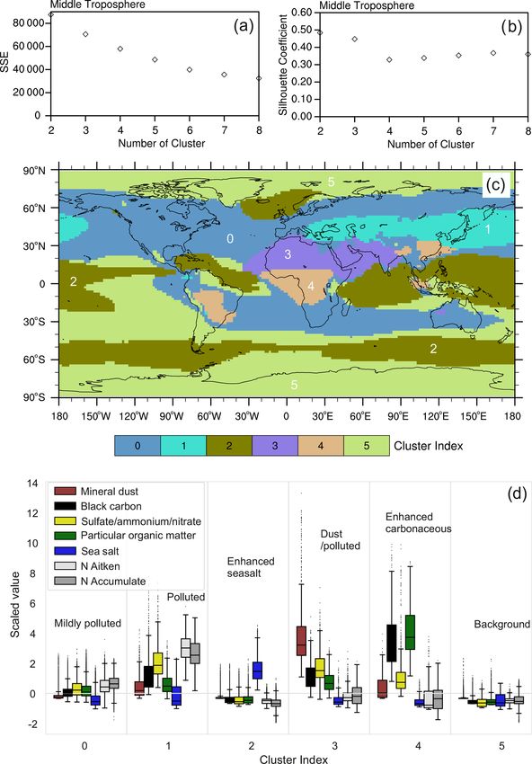
514                                                         J. Li et al.: An aerosol classification scheme for global simulations

additional statistical descriptions of the data distributions for    creases between k = 2 and k = 4, and reaches a roughly con-
individual aerosol parameters within each cluster. By com-           stant level at k = 5–11 (Fig. 2b). High SC value indicates that
paring the data distributions between individual aerosol pa-         the data within the cluster are similar and they are distinct
rameters and regimes we explicitly analyse the characteris-          from other clusters. The optimal solution is obtained by min-
tics of each regime.                                                 imizing SSE and maximizing the SC. Therefore, taking a bal-
                                                                     ance between small SSE and large SC, we limit the selection
3.1   Lower-tropospheric clusters                                    of k to 9 to 11. The difference between the 9-cluster and the
                                                                     10-cluster classification is that one oceanic aerosol regime in
For identifying lower-tropospheric clusters, the aerosol mass        the 9-cluster classification is further divided into 2 clusters in
and number concentrations from the global simulation are             the 10-cluster classification. The 11-cluster classification in-
vertically integrated from the Earth surface to the model layer      cludes a tiny regime that adds little information with respect
that corresponds to about 700 hPa. The resulting spatial dis-        to the 10-cluster one (Fig. S1 in the Supplement). We there-
tributions are shown in Fig. 1. High mineral dust column             fore choose k = 10 for the aerosol classification in the lower
masses (up to 1 × 10⁶ µg m−2 ) are simulated over the Sa-            troposphere.
hara and in other deserts, while values in other regions are            The resulting 10 aerosol regimes classified by K-means
mostly small (Fig. 1a). BC column masses are highest in              for the lower troposphere are displayed in Fig. 2c. These
South Asia and East Asia (up to about 3.5×10³ µg m−2 ), due          identified major aerosol classes match well with the expected
to anthropogenic pollution, and over Central Africa (about           regimes in this altitude range. Polar aerosols are classified in
2 × 10³ µg m−2 ) resulting from intense biomass burning ac-          cluster 0, while oceanic aerosols are roughly divided between
tivity (Fig. 1b). Peak values of the sea salt column masses          Northern Hemisphere and Southern Hemisphere by clusters
over the oceans range between 1 × 10⁴ and 2 × 10⁴ µg m−2             6 and 8, respectively. The large forests and savannas of Africa
(Fig. 1c). The pattern of POM columns closely follows that           and South America are covered by cluster 5 and cluster 1,
of BC, since the two species share similar emission sources          including major biogenic and fire aerosol sources (e.g. Den-
(Fig. 1d). Enhanced total masses of sulfate, nitrate, and am-        tener et al., 2006). Clusters 9 and 3 cover the main desert
monium (SNA) are noticeable, especially over south of the            regions over the Sahara and the Arabian Peninsula. Cluster
Eurasian continent (up to 5 × 10⁴ µg m−2 ) and the Arabian           9 marks the strong dust emission spots, while cluster 3 rep-
Peninsula (Fig. 1e), which could be due to coal burning              resents a kind of “background desert”, which shows slight
for energy production (Klimont et al., 2013), especially in          influences from aerosol transported from surrounding areas.
the case of India and China. Column-integrated numbers of            The regions characterized by strong anthropogenic pollution
Aitken mode particles, in the following called Aitken mode           (South Asia and East Asia) are assigned to cluster 7, while re-
number columns, are generally high in the Northern Hemi-             gions with moderate and low pollution are covered by cluster
sphere, with large values close to strongly polluted areas           4 and cluster 2, respectively, with the latter often extending
(Fig. 1f), while biomass burning largely contributes to the ac-      to oceanic regions possibly affected by long-range transport
cumulation mode number column, which is particularly high            of anthropogenic pollution from the continents.
in prominent biomass burning regions such as Central Africa             The characterization of the aerosol regimes in the lower
and South America (Fig. 1g). As expected, aerosol mass and           troposphere obtained with the K-means method can be fur-
number column show a large spatial variation in the lower            ther explored and interpreted using the boxplot in Fig. 2d.
troposphere, closely following the geographical distribution         The figure shows the distribution of samples collected within
of the main emission sources. This variability results in a          each regime and several statistical metrics, including maxi-
complex pattern of aerosol regimes, as shown below.                  mum, 75 % quantile, median, 25 % quantile, and minimum
   As explained in Sect. 2.3, K-means classifications are con-       of the standardized aerosol parameters that are not outliers.
ducted for a range of predefined cluster numbers k. The re-          We recall the use of multi-annual mean sample values and
sulting classification is coarse at low k, while increasing k        the consideration of column-integrated values in the lower-
leads to increased complexity. At some point, however, the           tropospheric column. The dots are outliers that can be ig-
added complexity of the K-means classification does not add          nored for statistical discussion. They are defined by ±1.5
further information and therefore a further increase of k is not     times the interquartile range of the data, which corresponds
useful. Hence, choosing a proper cluster number for the K-           to data beyond 2.67σ of a normal distribution. Note that val-
means analysis is not straightforward. Here, we use 10 clus-         ues on the y axis are the standardized values (calculated with
ters for the lower troposphere based on the K-means eval-            Eq. 5) but not the absolute value as shown in Fig. 1, in order
uation metrics (SSE and SC) and expert judgement, as de-             to do a proper classification with K-means and to compare
scribed above. SSE describes the sum of squared errors from          species with different units and scales. All aerosol proper-
each sample to the respective cluster centre (Eq. 3) and de-         ties within cluster 0 (polar regions) show lower values than
creases with increasing k. For the lower troposphere, SSE de-        in the other clusters, meaning that this can be considered
creases rapidly from k = 2 up to about k = 7 and then more           aerosol background, as also denoted in Fig. 2d. Low values
slowly for larger k (Fig. 2a). The SC is highest at k = 2, de-       are also found in clusters 6 and 8, with the exception of sea

Geosci. Model Dev., 15, 509–533, 2022                                                  https://doi.org/10.5194/gmd-15-509-2022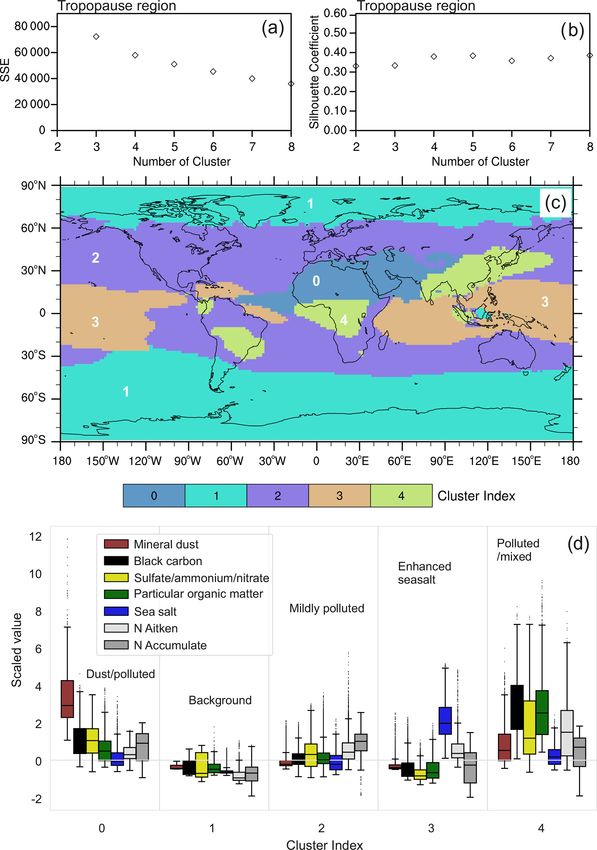
J. Li et al.: An aerosol classification scheme for global simulations                                                                  515

Figure 1. Simulated climatological aerosol properties for the lower troposphere (surface to ∼ 700 hPa), including vertically integrated mass
concentration of mineral dust (a), BC (b), sea salt (c), POM (d), and SNA (e) and the vertically integrated particle number concentration of
the Aitken mode Nakn (f) and accumulation mode Nacc (g).

salt, which has enhanced values. We therefore mark these                and South America and downwind areas and are character-
two clusters as oceanic aerosol. Clusters 6 and 8 are very              ized by enhanced POM, BC, and Nacc , which are all typi-
similar, which explains why they are merged into one clus-              cal indicators of strong biomass burning and biogenic activ-
ter if a 9-cluster (instead of 10-cluster) classification is used.      ity. The difference between the two clusters is that the en-
The difference between them is the slightly higher values of            hancement of these quantities is more pronounced in cluster
aerosol properties other than sea salt concentrations within            5 compared to cluster 1. This difference suggests that fresh
cluster 6, which points to a more polluted marine regime than           biomass burning and biogenic aerosol characterize cluster
in cluster 8, which represents remote oceanic regions. Clus-            5, while more aged particles are found in cluster 1 as a re-
ters 1 and 5 cover the major forests and savannas in Africa             sult of long-range transport and the subsequent dispersion

https://doi.org/10.5194/gmd-15-509-2022                                                        Geosci. Model Dev., 15, 509–533, 2022
516                                                              J. Li et al.: An aerosol classification scheme for global simulations

Figure 2. Lower-tropospheric clustering using K-means. The top row shows the evaluation metrics SSE (a) and SC (b) vs. a k range of
2–14. The middle row (c) highlights the spatial distribution of 10 aerosol regimes for the lower troposphere. The bottom row (d) shows
the data distribution of the seven considered aerosol properties within the 10 individual aerosol regimes and cluster names assigned to each
cluster based on the analysis of the aerosol data within the respective cluster. The boxplots describe the distribution of data by displaying five
statistical quantities that are not outliers: the maximum value (top whisker), 75 % quantile (top of box), median (middle line in box), 25 %
quantile (bottom of box), and minimum value (bottom whisker) of standardized aerosol parameters that are not outliers. The black dots are
outliers, defined as the data beyond 2.67σ of a normal distribution.

of the affected air masses in combination with particle wet                values for the other aerosol properties (in particular SNA and
and dry deposition. Cluster 9 and cluster 3 both show en-                  Nakn ) than cluster 3. This suggests that cluster 9 covers the
hanced mineral dust values, which agrees with their locations              regions of localized strong dust emissions, while cluster 3
in large deserts or in close proximity to desert regions. Clus-            includes dust-dominated air masses that are mixed with pol-
ter 9 shows much larger mineral dust values and much lower                 lution from other regions. The dominance of BC and SNA in

Geosci. Model Dev., 15, 509–533, 2022                                                          https://doi.org/10.5194/gmd-15-509-2022
J. Li et al.: An aerosol classification scheme for global simulations 517
cluster 7 matches well with the large pollution characterizing In the middle troposphere, the aerosol regimes are more
the South Asia and East Asia regions covered by this cluster. zonally uniform than lower down, but the lower troposphere
Cluster 7 also shows enhanced POM and number concentra- still has a very strong influence on the pattern (Fig. 4c).
tions in both Aitken and accumulation modes. We therefore The zonal uniformity particularly occurs in the case of clus-
name it the enhanced polluted Asian cluster. Clusters 2 and ters 0, 2, and 5 and appears to be related to the increas-
4 cover large parts of the Eurasian and American continental ing prevalence of zonal wind patterns in the middle tro-
regions. Cluster 4 is more polluted than cluster 2, but both posphere. Clusters 1, 3, and 4, on the other hand, show a
are relatively clean compared to other continental clusters stronger influence of the distribution of the emission sources
nearby (e.g. the strongly polluted Asian regions). We refer to and the transport patterns of the lower troposphere. The sta-
these clusters as moderately polluted continental and weakly tistical analysis of the aerosol properties within each clus-
polluted continental, respectively. Another important aspect ter allows the broad classification of clusters 2 and 5 as
worth noting is that continental aerosol clusters frequently middle-tropospheric background clusters and clusters 1, 3,
propagate into oceanic regions, showing that this method is and 4 as middle-tropospheric polluted clusters (Fig. 4d). The
also able to capture the long-range transport of pollutants lowest values of all aerosol properties are found in clus-
from the emission regions to the relatively clean marine en- ter 5, which can be classified as middle-tropospheric back-
vironment. For example, clusters 1, 2, and 3 also cover parts ground (relatively clean) and covers large fractions of the
of the central Atlantic Ocean, cluster 2 also appears over the Southern Hemispheric oceans and the polar regions. Clus-
Pacific Ocean near the west coast of the American continent, ter 2 is characterized by enhanced sea salt values, while
and cluster 4 extends over the north-western Pacific. the values of other aerosol species remain low, as in clus-
ter 5. Hence, the cluster includes background air enriched
with sea salt due to enhanced wind-driven emissions. Clus-
3.2 Middle-tropospheric clusters
ter 2 mainly covers the intertropical convergence zone (be-
tween 20◦ S and 20◦ N) with its strong updraughts and the
The clustering analysis for the middle-tropospheric layer Southern Hemispheric storm track area around 60◦ S, which
uses global aerosol data from about 700 to 300 hPa. As de- is also an uplift region between the mid-latitude cell and the
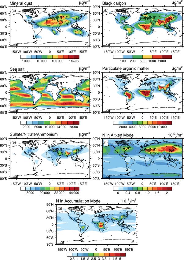
picted in Fig. 3, this altitude range shows lower values for polar cell of the main atmospheric circulation pattern. Due
the column mass and number concentrations (Fig. 1). For ex- to the strong upward transport in these regions, sea salt is
ample, the column mass of middle-troposphere mineral dust lifted from the sea surface to the middle troposphere. Cluster
(Fig. 3a) ranges from 2 × 10³ to 3.4 × 10⁴ µg m−2 in areas 0 is mainly located in the Northern Hemisphere and above
with prominent dust impact, compared to a range of 100 to the continents: it is characterized by mildly enhanced BC,
1 × 10⁶ µg m−2 in the lower troposphere (Fig. 1a). This is SNA, POM, Nakn , and Nacc . Similar enhancements of some
caused by the decrease of air density during upward trans- of these aerosol properties are evident in clusters 1, 3, and
port, by the dilution of the dust load due to mixing with dust- 4 but with much larger values. These clusters show simi-
free air masses, and by possible sinks due to wet deposition. lar aerosol characteristics and cover similar regions to their
A similar reduction is also evident in the other aerosol prop- counterparts in the lower troposphere (note, however, that
erties. The spatial distribution patterns, however, remain the the algorithm assigns different cluster index numbers for the
same between the middle troposphere and the lower tropo- lower- and middle-troposphere cases). These three polluted
sphere. However, the overall patterns, in many cases, show a clusters nicely identify three distinct sources: cluster 1 is
larger spatial extension that is caused by long-range transport mostly affected by the strong emission regions in South Asia
and dispersion of the respective air masses. and East Asia and Southern Europe and the Mediterranean
Due to this dispersion, a less complex clustering is re- Sea, cluster 3 presents a mixture of mineral dust and other
quired than in the lower troposphere. In general, we can pollution sources (with an evident prominence above large
expect k to decrease with increasing altitude due to the deserts), and cluster 4 is an enhanced carbonaceous and bio-
more uniform spatial aerosol distributions in the upper- genic cluster with significant coverage over biomass burning
atmospheric layers. For the middle troposphere, we evaluated and biogenic sources, e.g. in South America and Africa. It
K-means classifications with k = 2 to k = 8 using the same also occurs over East Asia, with its high anthropogenic emis-
metrics as applied above (Fig. 4a and b). As for the lower- sions of carbonaceous particles. Note that the scaled values
tropospheric case, SSE decreases with increasing k but more in Figs. 2d and 4d should not be compared directly among
slowly for k ≥ 6. The SC decreases to a minimum for k = 4 the different atmospheric layers because the input data for
and increases again to a stable level between k = 6 and k = 8. K-means analyses are scaled individually based on the data
The distribution of the major aerosol regimes becomes very within each layer.
robust at k = 6, while only minor regimes that do not show
prominent features are introduced at higher values. We there-
fore choose a six-cluster classification for the middle tropo-
sphere (see also Fig. S2 in the Supplement).
https://doi.org/10.5194/gmd-15-509-2022 Geosci. Model Dev., 15, 509–533, 2022518 J. Li et al.: An aerosol classification scheme for global simulations
Figure 3. The same as Fig. 1 but for the middle troposphere (from ∼ 700 to ∼ 300 hPa).
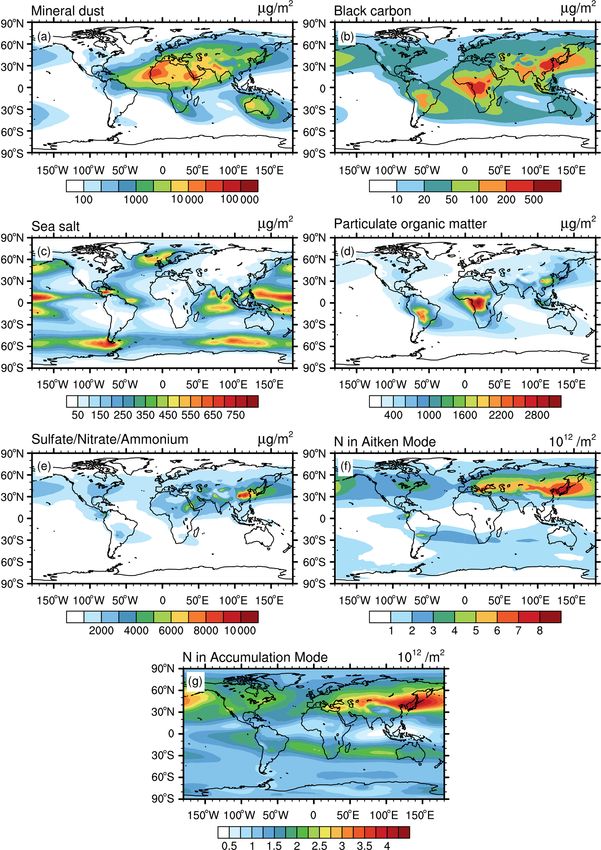
3.3 Tropopause region clusters eral dust mass column in the tropopause region amounts to
about 1 × 10³ µg m−2 , which is close to the minimum value
The clustering analysis for the tropopause region considers of mineral dust in the lower troposphere. Although aerosol
global aerosol data from about 300 to 100 hPa. The degree mass columns in the tropopause region are generally small
of spatial dispersion again increases when compared to the and a high degree of dispersion is reached, the spatial pat-
lower layers. Therefore, the distributions become more ho- terns for mineral dust, BC, POM, and SNA are still related
mogeneous than in the middle and lower troposphere (Fig. 5). to those in the lower troposphere. This demonstrates that lo-
The maximum values of the five aerosol mass columns cal upward transport of aerosols from the Earth’s surface
(mineral dust, BC, sea salt, POM, SNA) are lower in the to the tropopause region is efficient in areas showing en-
tropopause region (Fig. 5) than their background value in the hanced dust concentrations. However, this does not fully ap-
lower troposphere (Fig. 1). For example, the maximum min-
Geosci. Model Dev., 15, 509–533, 2022 https://doi.org/10.5194/gmd-15-509-2022J. Li et al.: An aerosol classification scheme for global simulations 519 Figure 4. The same as Fig. 2 but for the middle troposphere (from ∼ 700 to ∼ 300 hPa). ply to sea salt, which reaches high values only in the trop- that provides aerosol precursor gases, such as SO2 , leading ics corresponding to regions of strong convection over the to aerosol nucleation and growth favoured by the clean envi- oceans into the tropopause region (Fig. 5c). With regard to ronment of the tropopause region. the aerosol number columns, the effects of vertical and zonal As mentioned above and favoured by the homogeneous transport appear to be more complex. While the accumula- characteristics of aerosol in the tropopause region shown in tion mode particle number shows a similar behaviour to the Fig. 5, a more simplified clustering can be applied in this mass loadings, the Aitken mode particle number column ap- layer, reducing k to less than 6. Aerosol cluster distributions pears to be strongly influenced by new particle formation in for a range of different k are shown in Fig. S3 in the Sup- the tropopause region. Hotspots of the particle number par- plement. The SSE of K-means clustering for the tropopause ticularly occur over regions of enhanced gaseous pollution region (Fig. 6a) shows a similar structure to that in the mid- https://doi.org/10.5194/gmd-15-509-2022 Geosci. Model Dev., 15, 509–533, 2022
520                                                          J. Li et al.: An aerosol classification scheme for global simulations

Figure 5. The same as Fig. 1 but for the tropopause region (from ∼ 300 to ∼ 100 hPa).

dle troposphere (Fig. 4a), with noticeable convergence from            mostly covered by cluster 3. Clusters 0 and 4 cover a small
about k = 6. The SC reaches a maximum for k = 4 and k = 5              portion of the continents, including central Africa, the Sa-
(Fig. 6b). The combination of these two metrics suggests               haran region, and tropical and subtropical Asia. Figure 6d
k = 5 is the proper choice for the K-means classification for          highlights the aerosol characteristics for each cluster of the
the tropopause region. The resulting five clusters are shown           tropopause region. Cluster 1 shows the lowest values for all
in Fig. 6c. Large parts of the tropopause region belong to             aerosol properties which suggests that it should be character-
cluster 1, which covers both polar regions and most of the             ized as tropopause region background. Note that in the po-
southern extra-tropics. The second largest cluster is cluster          lar regions the pressure levels considered here are mostly lo-
2, which covers a large part of the northern extra-tropics and         cated in the stratosphere and therefore contain comparably
about half of the tropical ocean regions, with the other half          clean air. Cluster 3 shows similarly low values for all species

Geosci. Model Dev., 15, 509–533, 2022                                                    https://doi.org/10.5194/gmd-15-509-2022
J. Li et al.: An aerosol classification scheme for global simulations 521
except for sea salt, which is significantly enhanced due to up- ferent standardization methods summarized in Table 1. Fig-
ward transport in the intertropical convergence zone. Hence, ure 8a–e show the distribution of clusters resulting from the
we denote it as the tropopause region enhanced sea salt clus- differently scaled data and demonstrates how data scaling
ter. The slightly enhanced Nacc in cluster 3 relative to clus- changes the results of K-means clustering. Based on these
ter 1 is probably caused by new particle formation. Cluster results, we can draw the following four conclusions. (1) The
2 shows slight increases for all aerosol properties relative standardization that we use for this study (S1) simply scales
to cluster 1 but is still lower than in the other clusters. We the values of aerosol properties, but it does not change the
therefore define cluster 2 as the tropopause region mildly underling distribution of the raw data (see the first and sec-
polluted cluster. Cluster 0 features strongly increased mineral ond column in Fig. 7). (2) The most important criterion for
dust accompanied by slight increases in BC and SNA. There- K-means data preprocessing is that the data of different prop-
fore, it can be termed tropopause region dust/polluted cluster. erties should be scaled to a comparable range so that they are
This is also supported by its geographical location over the more or less equally weighted. This is clearly not achieved
Sahara and the Middle East, where mixtures of desert dust when using the standardization methods S4 and S5, lead-
with anthropogenic pollution could be expected. Cluster 4 ing to a large spread in the ranges of scaled data for dif-
shows strongly enhanced BC, SNA, and POM and mildly en- ferent aerosol properties (last two columns in Fig. 7). For
hanced mineral dust, which suggests that this regime should example, using the S4 method, the maximum scaled value
be termed the tropopause region polluted/mixed cluster. On of Nakn and Nacc is 1.0, while for the other five aerosol
the one hand, it is strongly influenced by the biomass burning properties the maximum values are smaller than 6.0 × 10⁻¹³
and biogenic aerosol sources over central Africa and South (Fig. 7, fifth column). Similarly, using the S5 method results
America. On the other hand, it also shows relevant coverage in much larger values for mineral dust compared to the other
over East Asia resulting from the strong pollution sources in aerosol properties (Fig. 7, sixth column). As a consequence,
these regions. Note that there are many similarities between the properties with larger values are weighted more strongly
the aerosol regimes of the tropopause region and the middle in the K-means clustering, leading to a classification largely
troposphere (Fig. 4), especially for clusters 3 and 4, which dominated by these properties (compare Figs. 1a and 8e). (3)
are largely controlled by efficient updraughts. Hence, these Both the S1 and the S3 methods scale the data to compara-
clusters also correspond well to lower-tropospheric aerosol ble ranges and retain the underlying distribution of the input
regimes with similar characteristics occurring in the same re- data, but S1 is more appropriate for this study. For exam-
gions (Fig. 2). ple, sea salt is a natural marine aerosol and its global range
of concentration values is relatively narrow in comparison to
the global ranges of other types of aerosols that have both an-
4 Discussion thropogenic and natural sources or pure natural sources but
with locally strong emissions as mineral dust. The maximum
4.1 Effects of scaling methods on K-means clustering values of global sea salt correspond to about 3 standard devi-
ations, while the maximum values of other aerosol properties
Since the choice of the variance applied for data scaling correspond to about 10–18 standard deviations (Fig. 7, sec-
could potentially have an effect on the clustering, we investi- ond column). This difference is a true feature of the data.
gate the influences of different scaling methods on our results Therefore, scaling sea salt and other aerosol properties to
in this section. Table 1 summarizes the five tested scaling the same range of values between zero and one using the S3
methods: S1 is the reference standardization method chosen method is not suitable for the purpose of this study since it
in this study. It is based on Eq. (6). S2 is similar to S1 but leads to comparably large weighting of sea salt. The differ-
applied to the base-10 logarithm of the input data. S3–S5 are ence in the resulting clusters using the S1 and S3 methods are
alternative methods based on different statistical metrics for depicted in Fig. 8: the S3 method (Fig. 8c) results in finer de-
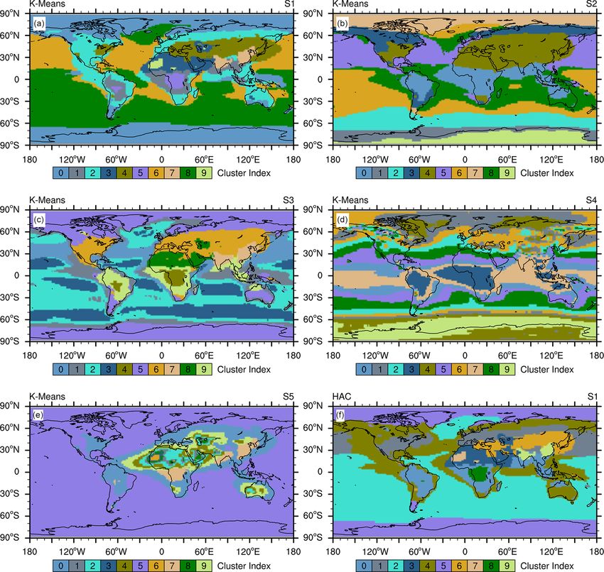
standardizing the data. The sensitivity test is applied to the fined clusters over the Southern Hemispheric ocean regions
data from the lower troposphere, as this domain is character- compared with S1 (Fig. 8a), but this is at the expense of a less
ized by a larger spatial variability than the middle- and upper- detailed clustering over the continental regions. For the pur-
atmospheric layers, hence more pronounced clustering fea- pose of this study, however, these fine-resolved oceanic clus-
tures can be expected. As an example, we use the 10-cluster ters are less relevant than a better-defined continental clus-
distribution. The optimal selection of k could vary among the tering. Furthermore, sharply defined Southern Hemisphere
different standardization approaches, but we choose a fixed clusters could also be achieved by increasing k using S1 data
value of k to analyse the impact on the results solely due (Fig. S1). (4) The “outliers” in the data distribution are im-
to the standardization method. The selection of an optimal portant for aerosol clustering. We tested this by applying the
value for k will be addressed again using a different approach base-10 logarithm to the original (skewed) distribution, re-
in the next section. sulting in a more Gaussian-like distribution (Fig. 7, third col-
Figure 7 compares the probability density functions umn) and thus removing the outliers. When applying the K-
(PDFs) of the raw input data and the scaled data using the dif- means algorithm with this method, several polluted clusters
https://doi.org/10.5194/gmd-15-509-2022 Geosci. Model Dev., 15, 509–533, 2022522 J. Li et al.: An aerosol classification scheme for global simulations Figure 6. The same as Fig. 2 but for the tropopause region (from ∼ 300 to ∼ 100 hPa). vanish (compare Fig. 8a and b). Although the basic structure ical data averaged over a long-term period (14 years), which of clusters is still visible, some important information is not already excludes unrepresentative high values in the aerosol captured with the S2 method. For the purpose of the present distribution. work, these high values in the data distribution should not Based on this sensitivity analysis, we conclude that the be interpreted as outliers in the general sense, i.e. indicating StandardScaler (S1) standardization method is the most ap- noise and incorrect information that could hinder K-means propriate one for the scope of this study. Although we focus clustering, but instead as features resulting from the intrin- in this section on the lower troposphere, this conclusion holds sically large spatial differences of aerosol properties across for the middle troposphere and tropopause region as well (see the globe, which provides useful information about the data Figs. S4–S7 in the Supplement). set. It is also important to recall that we consider climatolog- Geosci. Model Dev., 15, 509–533, 2022 https://doi.org/10.5194/gmd-15-509-2022
J. Li et al.: An aerosol classification scheme for global simulations 523
Table 1. Summary of the different scaling methods applied in this work.
Data Scikit-learn Definition Description of the scaled data Remarks
scaling Function
S1 StandardScaler Scaling the data of each feature Scaled data show a mean value of 0 Reference method chosen
(aerosol property) by subtracting its and a standard deviation of 1. in this study.
mean and dividing by its standard
deviation.
S2 StandardScaler Same as S1 but applied to the base- This removes the larger values from Demonstrates the impor-
10 logarithm of the input data. the tailed distribution of aerosol tance of using original (un-
properties. changed) data.
S3 MinMaxScaler Scaling the data of each feature by The values of all scaled properties Could be used here but is
subtracting its minimum and divid- range between 0 and 1. not as suitable as S1.
ing by its range.
S4 Normalizer Scaling the data by sample (not by The sum of squared features from a Not suitable for this study
feature) by applying Euclidian nor- sample (seven aerosol properties) is
malization. equal to 1.
S5 RobustScaler Scaling the data of each feature by The ranges of the scaled properties Not suitable for this study
subtracting its median and dividing are larger compared to other meth-
by its interquartile range. ods.
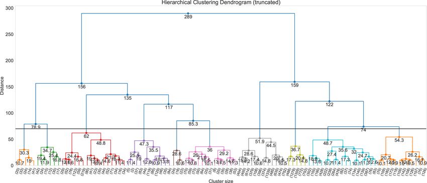
4.2 Comparison of K-means and HAC clustering ters (vertical axis) on the bottom of the hierarchy structure is
small but increases as the number of clusters decrease. At a
certain level, the dendrogram can be cut in correspondence
As with K-means, HAC clustering belongs to the family with the chosen number of clusters. This choice, however, is
of unsupervised clustering algorithms. It works with tech- also subjective and lies in the hand of the investigator. Our
niques based on hierarchical clustering schemes (e.g. Müll- selection of 10 clusters is supported by the dendrogram plot,
ner, 2013). More specifically, HAC treats all samples as in- which shows a distinct distance between clusters at this level
dividual clusters in the first step, and then it successively and is also consistent with the selection of 10 clusters for
merges the pair of clusters which are closest to each other in K-means clustering.
Euclidean distance until all samples are grouped into a single The cluster distribution of K-means and HAC shows a
cluster. In contrast to K-means, which requires a prescribed good overall agreement but also small differences (Fig. 8a
number of clusters k and separate metrics to evaluate a se- and f). We see similarities in the background clusters at the
lection of optimal k, HAC shows the hierarchy of clustering polar regions, the mildly polluted oceanic cluster at north-
along a workflow (the so-called dendrogram), which allows ern latitudes, the clean oceanic cluster at southern latitudes,
a selection of reasonable cluster numbers based on this hier- and the continental polluted clusters (dust cluster, biogenic
archical structure. cluster, Indian cluster, and southeastern China cluster). Dif-
In this section, we compare results of aerosol clustering ferences are visible, e.g. in the size of the biogenic cluster
with HAC and K-means, using the StandardScaler (S1) stan- over South America and the size of the mildly polluted conti-
dardization method and focus on the lower troposphere as nental cluster over the eastern USA. Interestingly, the extent
an example (additional results for the middle troposphere of biogenic clusters over Africa and other continental clus-
and tropopause region are provided in the Supplement). The ters over Europe and Asia seems to be identical in the two
way HAC clustering handles the data points is called link- cases. These fine differences in cluster size could be a result
age. There are different linkage methods, such as “Ward”, of K-means clustering the data by trying to separate samples
“Single”, and “Maximum”. Here we apply the Ward linkage in groups of equal variances, which HAC does not.
method for HAC clustering since it minimizes the sum of Another aspect to be considered when comparing these
squared differences within all clusters and is therefore sim- two clustering algorithms is the computational expenses. K-
ilar to the K-means approach. The truncated dendrogram of means is a fast algorithm. Its computing cost does not scale
HAC clustering for the lower-tropospheric aerosol is shown considerably with sample size or dimensions. HAC has a
in Fig. 9. It demonstrates the path from grouping all samples higher demand on computing time than K-means, especially
as individual clusters to one single cluster, and provides in- when the sample size is large. For a sample of size n, the
sights into the similarities and differences between individ- computing cost of HAC scales approximately as n2 (Das-
ual data points or clusters. The distance between two clus-
https://doi.org/10.5194/gmd-15-509-2022 Geosci. Model Dev., 15, 509–533, 2022You can also read