Seasonal distribution and drivers of surface fine particulate matter and organic aerosol over the Indo-Gangetic Plain
←
→
Page content transcription
If your browser does not render page correctly, please read the page content below
Atmos. Chem. Phys., 21, 10881–10909, 2021
https://doi.org/10.5194/acp-21-10881-2021
© Author(s) 2021. This work is distributed under
the Creative Commons Attribution 4.0 License.

Seasonal distribution and drivers of surface fine particulate matter
and organic aerosol over the Indo-Gangetic Plain
Caterina Mogno1 , Paul I. Palmer1,2 , Christoph Knote3 , Fei Yao1 , and Timothy J. Wallington4
1 School of GeoSciences, University of Edinburgh, Edinburgh, UK
2 NationalCentre for Earth Observation, University of Edinburgh, Edinburgh, UK
3 Model-Based Environmental Exposure Science (MBEES), Faculty of Medicine,

University of Augsburg, Augsburg, Germany
4 Research & Advanced Engineering, Ford Motor Company, Dearborn, MI 48121-2053, USA

Correspondence: Caterina Mogno (c.mogno@ed.ac.uk)

Received: 25 January 2021 – Discussion started: 4 February 2021
Revised: 24 May 2021 – Accepted: 18 June 2021 – Published: 20 July 2021

Abstract. The Indo-Gangetic Plain (IGP) is home to 9 %           OA (SOA), particularly over the lower IGP. We find that the
of the global population and is responsible for a large frac-    OA contribution to PM2.5 is significant in all four seasons
tion of agricultural crop production in Pakistan, India, and     (17 %–30 %), with primary OA generally representing the
Bangladesh. Levels of fine particulate matter (mean di-          larger fractional contribution. We find that the volatility dis-
ameter < 2.5 µm, PM2.5 ) across the IGP often exceed hu-         tribution of SOA is driven mainly by the mean total OA load-
man health recommendations, making cities across the IGP         ing and the washout of aerosols and gas-phase aerosol pre-
among the most polluted in the world. Seasonal changes in        cursors that result in SOA being less volatile during the pre-
the physical environment over the IGP are dominated by           monsoon and monsoon season than during the post-monsoon
the large-scale south Asian monsoon system that dictates         and winter seasons.
the timing of agricultural planting and harvesting. We use
the WRF-Chem model to study the seasonal anthropogenic,
pyrogenic, and biogenic influences on fine particulate mat-
ter and its constituent organic aerosol (OA) over the IGP        1   Introduction
that straddles Pakistan, India, and Bangladesh during 2017–
2018. We find that surface air quality during pre-monsoon        The Indo-Gangetic Plain (IGP), including parts of Pakistan,
(March–May) and monsoon (June–September) seasons is              India, and Bangladesh (Fig. 1), is one of the most populous
better than during post-monsoon (October–December) and           and polluted areas in the world. It is home to ∼ 700 mil-
winter (January–February) seasons, but all seasonal mean         lion people (9 % of the global population, Bangladesh Bu-
values of PM2.5 still exceed the recommended levels, so that     reau of Statistics, 2011; Indian National Commission on Pop-
air pollution is a year-round problem. Anthropogenic emis-       ulation, 2020; Pakistan Bureau of Statistics, 2017) and to the
sions influence the magnitude and distribution of PM2.5 and      associated sources of anthropogenic air pollution, which are
OA throughout the year, especially over urban sites, while       distributed proportionally to population, with hotspots over
pyrogenic emissions result in localised contributions over the   cities of various sizes from megacities of more than 10 mil-
central and upper parts of IGP in all non-monsoonal seasons,     lion people, e.g. Karachi, Lahore, Delhi, Kolkata, and Dhaka,
with the highest impact during post-monsoon seasons that         to smaller cities of a few million inhabitants, e.g. Faisal-
correspond to the post-harvest season in the agricultural cal-   abad, Patna, Kanpur, Lucknow, and Varanasi (DESA, 2018).
endar. Biogenic emissions play an important role in the mag-     It has been estimated that there would be a potential gain
nitude and distribution of PM2.5 and OA during the monsoon       in life expectancy in the IGP of approximately 4–6 years if
season, and they show a substantial contribution to secondary    levels of PM2.5 were reduced to standards set by the World
                                                                 Health Organisation (Greenstone et al., 2020; WHO, 2016).

Published by Copernicus Publications on behalf of the European Geosciences Union.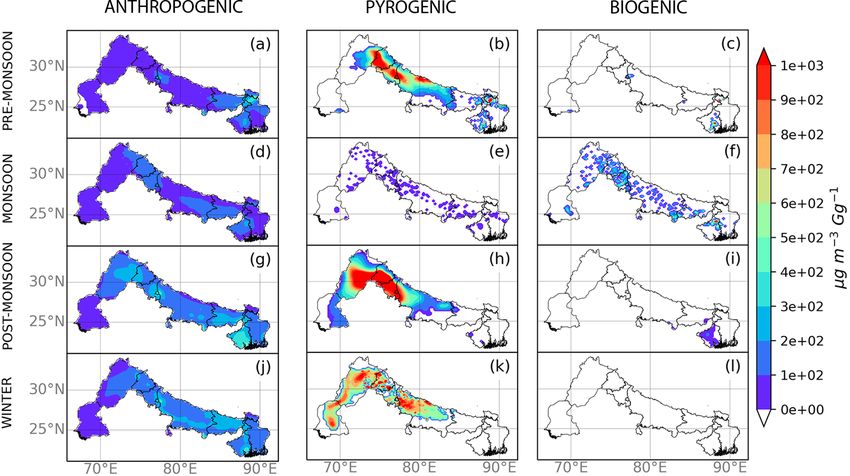
10882                                                                 C. Mogno et al.: Fine particulate matter over the IGP

The unique geography of the IGP and broader scale meteo-           2014). Intense agriculture over the IGP is associated with
rological drivers, coupled with the regional diversity of sea-     large emissions of ammonia, an aerosol precursor, from urea
sonal pollutant emission sources, makes this region one of         fertiliser application, as well as from post-harvest burning
the most challenging places to study the controls of its air       as described above (Kuttippurath et al., 2020; Wang et al.,
pollution and the consequent impact on human health. Here,         2020). Vegetation cover over the IGP consists mainly of
we use the WRF-Chem regional atmospheric chemistry and             croplands (Stibig et al., 2007; Gumma et al., 2019), which
transport model to describe the seasonal patterns of surface       have lower isoprene emissions than trees (Hardacre et al.,
organic aerosol and PM2.5 and to help disentangle the role         2013). Consequently, biogenic emissions over the IGP are
of anthropogenic, pyrogenic, and biogenic emissions in their       lower compared to other parts of south Asia (Guenther et al.,
surface patterns across the IGP.                                   2006; Stavrakou et al., 2014).
    The importance of the IGP lies in the fertility of its soils      Regional dispersion of air pollution over the IGP is dom-
formed from alluvium that is deposited across the Indus and        inated on a seasonal timescale by the monsoon system, in-
Ganges basins by the Indus and Ganges rivers. These rivers         fluenced by the high mountain ranges of Hindu Kush and
originate in the Himalaya mountains and the Tibetan Plateau.       Himalayas that lie to the northwest to northeast of the IGP.
The Indus and Ganges basins also benefit from precipita-           Agricultural planting and harvesting (and associated burn-
tion from the seasonal monsoon. The monsoon timing also            ing) are determined by the timing of the monsoon when the
defines the main seasons over the IGP (India Meteorologi-          majority of the annual rainfall falls. Consequently, observed
cal Department, 2020): the pre-monsoon season runs from            variations of PM2.5 reflect large-scale variations in meteorol-
March to May, the monsoon season is from June to Septem-           ogy and the seasonal variations in anthropogenic, biogenic,
ber, the post-monsoon season is from October to December,          and pyrogenic emissions (Jethva et al., 2005; Lelieveld et al.,
and winter occurs in January and February. The Indian states       2018; Schnell et al., 2018).
across the IGP (e.g. Punjab, Haryana, and Uttar Pradesh) rep-         A growing body of regional models have been used to
resent the vast majority of nationwide wheat and rice pro-         study the relationship between emissions, meteorology, and
duction. Rice and wheat are planted in May and November            PM2.5 over India (Kumar et al., 2015b; Bran and Srivas-
and harvested in October–November and April–May respec-            tava, 2017; Kulkarni et al., 2020; Ojha et al., 2020) and to
tively, following the rice–wheat cropping cycle. The IGP is        estimate the health impacts of outdoor exposure to PM2.5
also an important producer of sugarcane, cultivated mainly         (Ghude et al., 2016; Conibear et al., 2018; David et al., 2019).
in the Indus valley in Pakistan and in the Indian state of         Many studies have focused on post-monsoon biomass burn-
Uttar Pradesh. The two main seasons for planting are in            ing episodes and on air pollution during the winter season
September–October and February–March, followed by har-             over the upper-central Indian part of the IGP (Guttikunda
vesting during the winter and pre-monsoon months, respec-          and Gurjar, 2012; Ram et al., 2012; Pant et al., 2015; Kumar
tively. Crop residues left from harvesting, e.g. husk, bran, and   et al., 2015a; Jethva et al., 2018; Singh et al., 2018; Krishna
straw, are generally burned in open fires. Traditionally, these    et al., 2019; Mhawish et al., 2020). But of course the IGP
residues were ploughed back into the soil to maintain fer-         also includes parts of Pakistan and Bangladesh that remain
tility and stability, but the sheer scale of current production    poorly studied, even though they are connected via atmo-
precludes these practices in time for a second growing season      spheric transport. With only a few exceptions, these studies
(Chauhan et al., 2012; Ahmed et al., 2015). Open burning of        have focused on total PM2.5 , although there is evidence that
these residues across the IGP, particularly during the post-       single aerosol components play a major role in PM2.5 compo-
monsoon season, is a large source of gaseous and particulate       sition over the IGP (Gani et al., 2019 and Singh et al., 2018,
pollution that has implications for regional air quality and hu-   and references therein). Measurements have shown that or-
man health (Vadrevu et al., 2011; Jethva et al., 2019; Sembhi      ganic aerosol (OA), originating from anthropogenic, pyro-
et al., 2020). Residential biofuel combustion also plays an        genic, and biogenic emissions, constitutes a significant frac-
important role in air quality (Conibear et al., 2020; Agarwala     tion (20 %–35 %) of PM2.5 across the IGP, especially during
and Chandel, 2020).                                                post-monsoon and winter seasons (Ram et al., 2008; Alam
    The high population density and intense human activity         et al., 2014; Rajput et al., 2014; Behera and Sharma, 2015;
over the IGP result in anthropogenic emissions being a ma-         Sharma et al., 2016). OA exists as a complex mixture, com-
jor source of regional surface air pollution (Begum et al.,        prising of thousands of individual organic compounds, and it
2013; Guttikunda and Jawahar, 2014; Shahid et al., 2015;           is made up of primary OA (POA), emitted directly to the at-
Venkataraman et al., 2018). Residential energy consumption         mosphere, and of secondary OA (SOA), formed by the con-
represents a major contribution to anthropogenic emissions,        densation of organic vapours as they become progressively
with a large fraction of the rural and urban population us-        less volatile through oxidation (Seinfeld and Pandis, 2016;
ing solid fuel for cooking (Conibear et al., 2018). Emissions      Donahue et al., 2006). Changes in OA volatility are key for
from land transportation, particularly in cities, also represent   the formation of SOA, and it is particularly sensitive to tem-
a significant contribution to anthropogenic emissions (Be-         perature, ambient concentration of OA, and nitrogen oxide
gum et al., 2013; Guttikunda et al., 2014; Mallik and Lal,         levels (Shrivastava et al., 2017). We take advantage of the

Atmos. Chem. Phys., 21, 10881–10909, 2021                                          https://doi.org/10.5194/acp-21-10881-2021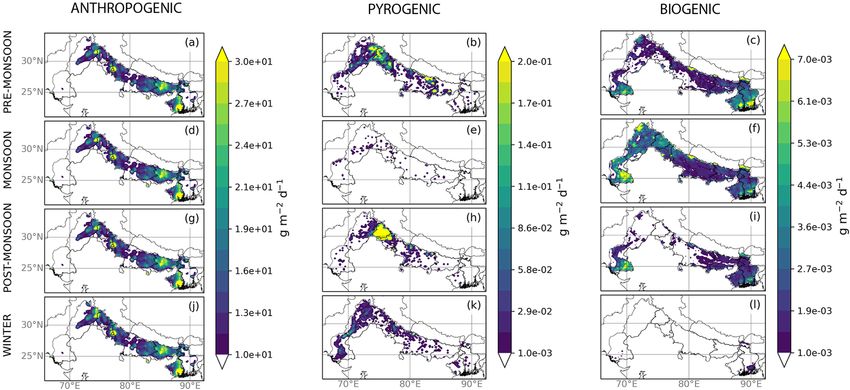
C. Mogno et al.: Fine particulate matter over the IGP 10883
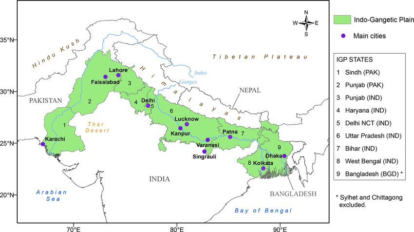
Figure 1. Geographical and administrative features of the Indo-Gangetic Plain (IGP), including Pakistan, India, and Bangladesh. Numbers
denote individual IGP states, and purple dots denote the main cities.
volatility basis set (VBS) model, which helps to describe suc- genic emissions on the atmospheric distribution of PM2.5 and
cinctly the evolving volatility of OA through oxidative chem- OA over the IGP.
istry in the atmosphere (Donahue et al., 2006, 2012; Chuang
and Donahue, 2016), described below. This method has been 2.1 Weather Research and Forecasting model coupled
used successfully in a range of modelling studies (Lane et al., with Chemistry
2008b; Bergström et al., 2012; Ahmadov et al., 2012; Zhang
et al., 2013; Zhao et al., 2016). We use v.3.9.1.1 of the Weather Research and Forecasting
We use the WRF-Chem regional atmospheric chemistry (WRF) model coupled with Chemistry (WRF-Chem) (Grell
model to characterise the seasonal and spatial distributions et al., 2005) to describe the emissions and atmospheric chem-
and composition of PM2.5 and OA in light of synoptic me- istry and transport associated with gas- and aerosol-phase
teorology and emission drivers over three subregions of the compounds over the IGP during 2017 and 2018. WRF uses
IGP, including relevant parts of Pakistan and Bangladesh. We the Advanced Research WRF (ARW) dynamical solver to
use a 1-D VBS model to describe the evolution of OA and solve the fully compressible, non-hydrostatic Euler equations
its influence on PM2.5 , described in Sect. 2. In Sect. 2, we that describe atmospheric flow. These calculations are cou-
also describe the in situ and satellite measurements we use to pled with atmospheric chemistry, so that our PM2.5 and OA
evaluate our model. In Sect. 3, we describe the seasonal me- calculations are consistent with the meteorology.
teorology over the IGP, the seasonal distributions and compo- Our study domain is defined as 17–40◦ N and 64–97◦ E,
sition of PM2.5 and OA, and the seasonal distribution of SOA encompassing the IGP at a horizontal spatial resolution of
volatility. In Sect. 3, we also use a perturbative approach to 20 km and using 33 vertical levels that span from the sur-
understand the sensitivity of PM2.5 constituent distributions face to 50 hPa (' 19 km). For the description of terrain
to changes in anthropogenic, pyrogenic, and biogenic emis- data for the domain (land-use and soil categories), we use
sions and to seasonal changes in the atmospheric environ- MODIS IGPB 21-category data at 30 arcsec resolution (∼
ment. We conclude our study in Sect. 4. 1 km) (Friedl et al., 2010). To define our initial conditions
and lateral boundary conditions, and for nudging (New-
tonian relaxation), we use meteorological reanalyses from
NCEP FNL Operational Model Global Tropospheric Anal-
2 Data and methods yses Data (National Centers for Environmental Prediction,
National Weather Service, NOAA, U.S. Department of Com-
Here, we describe the WRF-Chem model that we use to un- merce, 2015) at a spatial resolution of 0.25◦ × 0.25◦ and at a
derstand the influence of anthropogenic, pyrogenic, and bio- temporal resolution of 6 h. We use the nudging approach at
https://doi.org/10.5194/acp-21-10881-2021 Atmos. Chem. Phys., 21, 10881–10909, 2021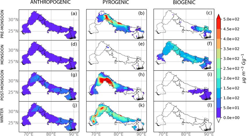
10884                                                                      C. Mogno et al.: Fine particulate matter over the IGP

Figure 2. Seasonal mean daily emissions over the IGP (g m−2 d−1 ) of (a, d, g, j) anthropogenic, (b, e, h, k) biomass burning, and (c, f,
i, l) biogenic (isoprene) emissions. Anthropogenic emissions from EDGAR-HTAP and fire emissions from FINN. Biogenic emissions are
calculated online in WRF-Chem using MEGAN. To determine total anthropogenic and pyrogenic emissions, we sum across all emitted
species, respectively, while for biogenic emissions, we consider only isoprene.

all levels to prevent our calculations from deviating too far          The log10 C ∗ = −4 volatility corresponds to an inert com-
from observed meteorology. Table B1 provides more details              pound and serves computationally as a loss of particle-phase
about the meteorological processes we use in our calcula-              organics to avoid unrealistic volatile mixtures due to contin-
tions. Chemical initial conditions and lateral boundary condi-         uously ageing of gas-phase SVOCs. Lumped anthropogenic,
tions for each month are provided by 6-hourly CAM-CHEM                 pyrogenic, and biogenic gas-phase aerosol precursors un-
global model data (Buchholz et al., 2019). We spin up each             dergo continuous gas-phase oxidation and partition between
simulation for a week before studying the model output to              the gas and aerosol phase using pseudo-ideal partitioning the-
minimise the influence of the initial conditions.                      ory (Pankow, 1994). Partitioning between the gas and aerosol
   To describe gas-phase chemistry, we use the Model for               phase depends on total organic aerosol load and temperature.
OZone And Related chemical Tracers, version 4 (MOZART-                 SOA yields are also dependent on NOx levels, so SOA yields
4) chemical mechanism (Emmons et al., 2010), including                 are calculated differently for low- and high-NOx conditions,
the extended treatment of volatile organic compound (VOC)              through a branching ratio (Lane et al., 2008a). We also in-
chemistry (Knote et al., 2014). Photolysis rates are calculated        clude the SOA formation from glyoxal (Knote et al., 2014).
by the Fast Tropospheric Ultraviolet–Visible (FTUV) mod-               Loss of SVOCs is from washout via convective- and grid-
ule (Tie et al., 2003).                                                scale precipitation. Our chosen implementation of VBS only
   We use the Model for Simulating Aerosol Interactions and            accounts for SVOCs and assumes that POA is inert, so that it
Chemistry (MOSAIC) to simulate aerosols chemistry (Za-                 contributes only to the aerosol mass. We do not include direct
veri et al., 2008), including aqueous-phase chemistry (Knote           emissions of SVOCs or intermediate VOCs (IVOCs). This
et al., 2014). MOSAIC describes aerosols using four sec-               is a limitation of our current implementation given evidence
tional discrete size bins: 0.039–0.156, 0.156–0.625, 0.625–            that SVOC and IVOC vapours create a considerable amount
2.5, and 2.5–10 µm. The first three of these bins represent            of regional SOA and that POA emissions are semivolatile
PM2.5 , while the largest one describes coarse particulate mat-        and undergo oxidation and should also be considered in de-
ter (PM2.5−10 ). We use the 1-D VBS method to describe SOA             scribing SOA production (Robinson et al., 2007). To describe
for WRF-Chem (Knote et al., 2015), based on previous stud-             POA using the VBS approach, we would require information
ies (Lane et al., 2008b; Ahmadov et al., 2012). For each of the        about the volatility distribution of POA, but conventional in-
four aerosol size bins in MOSAIC, the 1-D VBS implemen-                ventories typically consider POA to be non-volatile. The 1-D
tation considers five volatility bins for semi-volatile organic        version of the VBS model is unable to describe some aspects
compounds (SVOCs), described by effective saturation con-              of SOA formation, including fragmentation and the increase
centrations C ∗ of 10−4 , 1, 10, 100, and 103 µg m−3 at 298 K.         in OA oxidation state, which are better described by the 2-D

Atmos. Chem. Phys., 21, 10881–10909, 2021                                               https://doi.org/10.5194/acp-21-10881-2021
C. Mogno et al.: Fine particulate matter over the IGP                                                                        10885

version of the model that tracks the oxygen-to-carbon ratio         Gases and Aerosol from Nature (MEGAN; Guenther et al.,
(O : C) in addition to organic mass (Donahue et al., 2012).         2006).
Previous studies have shown that the 2-D VBS model im-                 Figure 2 shows the seasonal distributions of total anthro-
proves model–measurement agreement in SOA (e.g. Zhao                pogenic, pyrogenic, and biogenic (predominately isoprene)
et al., 2016) but has a significant associated computational        emissions over the IGP. Total anthropogenic emissions have
burden when used in 3-D chemistry transport models. Fur-            been calculated by summing the mass contribution from all
ther details of this VBS implementation in WRF-Chem are             the chemical species (gas and particle) specified in the in-
described in Knote et al. (2015) and references therein.            ventory once preprocessed onto the model domain using the
   We use monthly anthropogenic emissions from Emission             WRF-Chem tools for the community (ACOM-NCAR, 2020).
Database for Global Atmospheric Research with Task Force            We converted gas emissions to mass units using the appro-
on Hemispheric Transport of Air Pollution (EDGAR-HTAP               priate molar mass for each species. The same approach has
v2.2) for the year 2010 (Janssens-Maenhout et al., 2015) as         been used to calculate fire emissions, while isoprene emis-
provided by the WRF-Chem community, which provides the              sions are calculated online by MEGAN in the WRF-Chem
total anthropogenic emissions and includes a non-methane            model and then converted to mass units. Anthropogenic
volatile organic compound (NMVOC) speciation accord-                emissions generally dominate in all seasons (Fig. 2a, d, g,
ing to the gas and aerosol chemistry scheme we use here             j), with daily values ranging from 101 to 102 g m−2 d−1 .
(MOZART-MOSAIC). Using an anthropogenic emission in-                The two largest localised regions of anthropogenic emissions
ventory for 2010 to describe atmospheric chemistry dur-             are Delhi and Kolkata with emissions > 100 g m−2 d−1 , fol-
ing 2017–2018 will inevitably introduce some biases in our          lowed by smaller Indian cities, e.g. Patna, Varanasi, Kan-
model PM2.5 estimates, particularly because our study do-           pur, and Lucknow (Fig. 1). Just south of the border of Ut-
main includes regions with rapidly growing emissions. From          tar Pradesh, the Madhya Pradesh district of Singrauli hosts
2010 to 2017, India has seen reductions in black carbon (BC),       several large power plants. The Pakistani and Bangladeshi
organic carbon (OC), CO, and NMVOC emissions from                   parts of the IGP generally have the lowest anthropogenic
the residential sector, owing to policies that have enabled a       emissions, with the exception of Karachi in south Pakistan,
switch to cleaner residential fuels and energy sources. How-        the north Pakistani Punjab (the most populated part of Pak-
ever, India’s growing economy had led to a rapid increase           istan where Lahore and Faisalabad are located), and Dhaka in
of NOx and SO2 emissions from the industrial sector (∼              Bangladesh. Emissions from Karachi and Dhaka have lower
+12 %, ∼ +10 %) and energy sector (∼ +20 %, ∼ +26 %)                emissions per capita than Indian cities of comparable size.
and an increase in NOx and NMVOC from on-road trans-                   Fires have a strong seasonal cycle, peaking during pre-
portation (∼ +50 %, ∼ +27 %). An increase in intensive              monsoon and post-monsoon seasons (Fig. 2b, h), with emis-
agricultural practices over the Indian IGP has increased am-        sions ∼ 10−1 g m−2 d−1 , mainly due to agricultural stubble
monia emissions (NH3 ; ∼ +15 %) (McDuffie et al., 2020).            burning. The post-monsoon harvesting season includes fire
Errors in PM precursor gaseous emissions will impact our            emissions rates that are 3 times higher compared to the pre-
ability to describe air pollution for our study year, especially    monsoon season (∼ 0.3 and ∼ 0.9 g m−2 d−1 , respectively).
for individual components of secondary inorganic aerosols           Post-monsoon fires are almost exclusively located in the In-
(nitrate, sulfate, and ammonium) and SOA. It remains diffi-         dian Punjab, with the largest values at the border with the
cult to disentangle the impact of using outdated emission es-       state of Haryana. Pre-monsoon fires are located around the
timates from other sources of model error, e.g. meteorology,        border of Pakistani and Indian Punjab and upper Haryana.
chemistry, land-use change, and model resolution. For pyro-         There are also some isolated fires in the eastern part of the
genic emissions, hourly biomass burning emissions are taken         IGP. During winter (Fig. 2k), low fire activity is present in
from the Fire Inventory from NCAR (FINNv.15) inventory              the Indus valley in Pakistan and mainly over Uttar Pradesh
for 2017–2018 (Wiedinmyer et al., 2011). Pyrogenic emis-            from the post-harvesting of sugarcane crops.
sions are apportioned between FINN and EDGAR-HTAP                      Biogenic emissions peak during pre-monsoon and mon-
inventories. The FINNv1.5 inventory includes global esti-           soon seasons (Fig. 2c, f), with values of 2 × 10⁻³ and 1.5 ×
mates of trace gas and particle emissions from the open burn-       10−2 g m−2 d−1 , respectively. The largest values are over
ing of biomass, which includes wildfire, agricultural fires,        Sindh in Pakistan, West Bengal, and Bangladesh. Land cover
and prescribed burning (Wiedinmyer et al., 2011). EDGAR-            over the IGP is dominated by croplands, but the state of
HTAPv2.2 is focused on anthropogenic emissions but ex-              Sindh includes coastal mangrove plantations, inland riverine
cludes large-scale biomass burning (e.g. forest fires, peat         forests, irrigated plantations, and rangelands (Ministry of En-
fires), agricultural waste, or field burning. Within its residen-   vironment Government of Pakistan, 2009). Moreover, West
tial sector, emissions include small-scale combustion, includ-      Bengal and Bangladesh emissions are mostly confined close
ing heating, lighting, cooking, and solid waste disposal or in-     to the coast, where forest land is present (Reddy et al., 2016).
cineration (Janssens-Maenhout et al., 2015). Biogenic emis-         During these two seasons, there are also isoprene emissions
sions are calculated online using the Model of Emissions of         over Uttar Pradesh from forests in Pilibhit and Kheri and
                                                                    from northeast Pakistan.

https://doi.org/10.5194/acp-21-10881-2021                                         Atmos. Chem. Phys., 21, 10881–10909, 2021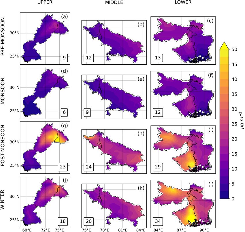
10886                                                                      C. Mogno et al.: Fine particulate matter over the IGP

   For computational expediency, we have chosen a represen-          the base run b Cij, b . The change in concentration in each
                                                                                            t
tative period of 1 month for each distinct season over the IGP.      grid cell is therefore scaled by the same 1E, allowing local
We define, based on the seasonal definition of the Indian Me-        and non-local emission influences to be considered equally
teorological Department (India Meteorological Department,            and to avoid singularities in grid cells where there is no net
2020), the pre-monsoon period as 18 April to 16 May 2017,            emission change. We use this scaling because it allows us
the monsoon season as 3 to 31 July 2017, the post-monsoon            to compare the sensitivity of atmospheric concentrations to
season at 18 October to 16 November 2017, and finally win-           different sources types. 1E is calculated as the difference of
ter as 8 January to 5 February 2018. The 2017–2018 year is           total emissions within the IGP domain between the perturbed
close to the climatological mean state, so our results are typ-      model run and the base model run for a given source type.
                                                                                                                                        p
ical of this region rather than being influenced by significant         Total emissions across the IGP for the perturbed run Etot
circulation changes due to, for example, El Niño–Southern            and for the base run Etot  b are calculated by summing emis-

Oscillation climate variations (Null, 2020).                         sions from all species for the length of the simulation and for
   For the purposes of reporting our results, we divide the          all grid cells across the IGP. In more detail, emissions at each
IGP into three subregions: the upper IGP that includes the           grid point ij for species s between two consecutive model
Pakistani states of Sindh and Punjab and the Indian Punjab;          outputs at t and t + 1 are calculated (for both the perturbed
the middle IGP that includes the Indian states of Haryana,           and base runs) by Eij, t, s = ij, t, s 1tAij . ij, t, s denotes the
Delhi NCT, and Uttar Pradesh; and the lower IGP that                 emission rate of species s at location ij and output time t, Aij
includes the Indian state of Bihar and West Bengal and               denotes the area of grid point ij , which in our calculations
Bangladesh, excluding the states of Chittagong and Sylhet            is constant at 400 km2 , and 1t corresponds to an interval of
(Fig. 1).                                                            model output, which in our calculation is 3 h. To take into ac-
                                                                     count the different spatial variability of emissions from dif-
2.2   Determining the sensitivity of PM2.5 and OA to                 ferent sources (Fig. 2), we scale 1E with the total number of
      changes in precursor emissions                                 grid cells within the IGP for which the emission difference is
                                                                     > 0.001 g m−2 d−1 , corresponding approximately to cumu-
We use a perturbative approach to determine the importance           lative emissions > 2.8 Mg for each grid cell in 1 week. This
of different source sectors on PM2.5 and OA, which takes into        threshold corresponds to a lower limit for significant emis-
account the non-linear chemical environment. Alternatively,          sions rate across the area considered (Fig. 2). We also neglect
setting a particular emission source to zero would result in a       values of Sij for which the change in the pollutant concen-
significant non-linear response that is unique to the source,        tration Cij < 5 % of mean pollutant seasonal concentration
consequently precluding any meaningful comparison of the             over the IGP (4 µg m−3 and 1 for PM2.5 and total OA, respec-
importance of a particular source to PM2.5 and OA.                   tively). Using this additional threshold allows us to isolate
   First, we run a base run for each season. We then, for each       significant changes in concentrations due to direct changes
season, systematically perturb one emission source by +5 %           in emissions and remove smaller values due to model non-
over the study domain for the central week of each season,           linearity. We report the sensitivity parameter Sij with units
keeping the other sources the same as the base run. Finally,         of micrograms per cubic metre per gigagram (µg m−3 Gg−1 ).
we calculate the sensitivity Sij of species concentration to the     In a policymaking context, our sensitivity parameter provides
changes in a given source of emissions as                            information about how to control atmospheric concentrations
                             P p                 b
                                                                     by changing different emission sources in order to obtain the
      1Cij    1Cij               t (Cij, t − Cij, t )                highest air quality benefits from certain emission reductions.
Sij =      = p      b
                        =P            p            b
                                                             , (1)
      1E    Etot − Etot    ij, t, s (Eij, t, s − Eij, t, s )
                                                                     2.3    Data used for model evaluation
where 1Cij represents the concentration change of our target
species (PM2.5 and OA in this study) at grid point ij in re-         We use in situ measurements of PM2.5 , PM10 , CO, NO2 , O3 ,
sponse to an emission change 1E summed over the IGP for              and SO2 from the Indian Central Pollution Control Board
a particular source. We perturb directly anthropogenic and           (CPCB, 2020) and PM2.5 data collected atop the US Em-
fire emissions rates. Biogenic emissions are calculated online       bassy in Pakistan and Bangladesh (U.S. Department of State,
by scaling normalised emission rates by factors that describe        2020). We accessed these data from the OpenAQ platform
changes in, for example, temperature, photosynthetic active          (OpenAQ, 2020). Appendix B describes an overview of the
radiation, and leaf area index (LAI) (Guenther et al., 2006).        in situ data, our data cleaning approach, and evaluation met-
We modify the WRF-Chem code to increment only isoprene               rics. Given the lack of continuous measurements of OA and
emissions because our calculations suggest they account for          its components POA and SOA over the IGP, we compare
almost all of biogenic emissions over the IGP, in agreement          our model OA with measurements available from the liter-
with other studies (Singh et al., 2011; Surl et al., 2018). 1Cij     ature. We also evaluate the model using satellite observa-
is calculated by summing over time the difference in concen-         tions of aerosol optical depth (AOD) from the NASA Moder-
                                                         p
trations at each grid cell ij of the perturbed run p Cij, t and      ate Resolution Imaging Spectroradiometer (MODIS) instru-

Atmos. Chem. Phys., 21, 10881–10909, 2021                                             https://doi.org/10.5194/acp-21-10881-2021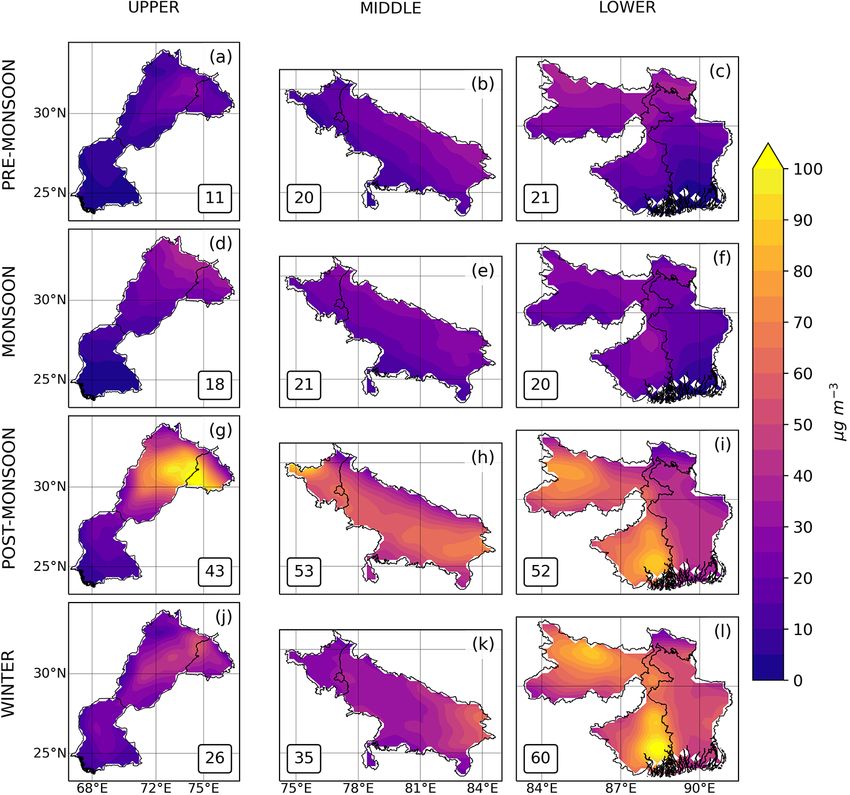
C. Mogno et al.: Fine particulate matter over the IGP                                                                      10887

ment aboard the Terra and Aqua satellites, which have a lo-       study period (2017–2018), so we instead use data from 2019
cal equatorial overpass time of 10:30 and 13:30, respectively.    for the monsoon and post-monsoon seasons and data from
AODs are retrieved at 550 nm, corresponding to particle sizes     2020 for the winter and pre-monsoon seasons, which rep-
of 0.1–2 µm and comparable to the PM2.5 size range. In par-       resents an additional source of error. Previous studies show
ticular, we use the MODIS Collection 6.1 Level 2 combined         that regional modelling over south Asia tends to overestimate
Dark Target and Deep Blue AOD product, available on a             satellite column observations of NO2 by 10 %–50 % over the
10 km spatial resolution (Levy et al., 2013).                     Indo-Gangetic Plain, the bias peaking as high at 90 % dur-
   Here we summarise the main results of our evaluation (de-      ing winter months (Kumar et al., 2012b) and up to +131 %
tailed results are available in Appendix B). We report the nor-   when compared to ground-based observations over densely
malised mean bias (NMB) and the Pearson correlation coef-         populated urban regions (Karambelas et al., 2018). These dif-
ficient r, which we use to describe how well the model repro-     ferences have been attributed mainly to errors in NOx emis-
duces the observations. The model tends to overestimate sur-      sion inventories over densely populated areas, uncertainties
face PM2.5 concentrations (0.004 < NMB < 0.4), especially         in seasonal variations of emissions, absence of diurnal and
during monsoon season (NMB = 0.4), but it has skill in re-        vertical profiles of anthropogenic emissions (Kumar et al.,
producing observed seasonal variations (r > 0.62), with the       2012b; Karambelas et al., 2018), and underestimation of pre-
exception of the monsoon season (r = 0.09). Poorer model          cipitation rate that will reduce the loss of soluble trace gases
performance during the monsoon period may be due to a             (Kumar et al., 2012a). Similarly, previous regional model
number of compounding factors. In particular, it is challeng-     studies of the IGP region have tended to over-predict con-
ing to reproduce observed atmospheric water vapour and pre-       centrations of SO2 , with NMB > 3.5 (Conibear et al., 2018;
cipitation over the Bay of Bengal, western coasts of India,       Kota et al., 2018). We attribute our positive model bias of
and the Himalayan foothills during summer months. Uncer-          SO2 to using an outdated emission inventory that does not
tainties in the representation of topography; insufficient mix-   take into account the beginning of a shift from coal- to gas-
ing in the boundary layer; errors in moisture transport, simu-    based power plants (Sharma and Khare, 2017). Urbanisation
lation of surface moisture availability, and soil temperature;    has been shown to affect the diurnal spatial distribution of
and an excessive water vapour flux from the ocean all con-        surface ozone (Li et al., 2014, and references therein) and
tribute to model error (Kumar et al., 2012a). Previous stud-      also the magnitude and location of anthropogenic emissions
ies have shown that monsoonal rainfall is not well described      of NOx and VOCs that subsequently affect surface ozone
by regional models such as MM5 or WRF (Rakesh et al.,             photochemistry (Zhang et al., 2004; Ghude et al., 2013). Fi-
2009; Ratnam and Kumar, 2005). When we compare our                nally, some fraction of the overestimation of surface ozone
WRF model simulation with MERRA-2 reanalysed meteo-               is linked to our use of the MOZART chemical mechanism
rology (Gelaro et al., 2017), we find that precipitation rates    that has been previously reported to have a positive model
have a negative model bias of ' 80 % over the IGP, similarly      bias over south Asia compared to other mechanisms (Sharma
to what Conibear et al. (2018) obtained with a similar model      et al., 2017). Collectively, these model limitations associated
set-up.                                                           with describing reactive trace gases will impact our ability to
   For PM10 , the model tends to underestimate the obser-         model particulate matter, especially secondary components
vation in all seasons (NMB up to −0.25), except in the            over urban areas across the IGP. For OA, the model repro-
pre-monsoon season (NMB = 0.15), and has poorer skill in          duces the order-of-magnitude seasonal trends (Table B4),
reproducing observed PM10 variations compared to PM2.5            but additional measurements are needed to robustly assess
(r ≤ 0.69), especially during winter and the pre-monsoon          model performance. Table B5 shows that WRF-Chem AOD
season. We generally find poorer model agreement with gas-        agrees with spatial distributions of MODIS AODs, with r
phase pollutants, including a positive model bias and com-        typically > 0.5 with the exception of the monsoon season
paratively poor correlations with observations of NO2 , SO2 ,     (r = 0.35). Poor model skill during the monsoon season may
and O3 (Table B3). We attribute this to multiple sources of       reflect difficulties in retrieving AOD during extensive sea-
error. Given the coarse spatial and temporal resolution our       sonal cloud coverage. In addition, the model has specific
model (20 km × 20 km spatial, 3 h temporal), we expect our        difficulties in reproducing atmospheric aerosol abundances
model to be affected by non-negligible representation error       during monsoon season, as highlighted earlier in this sec-
due to the CPCB network sites often being located near to         tion, that could affect the simulated total AOD column. The
roadsides or in dense urban areas where the model will strug-     model tends to overestimate MODIS AOD during the pre-
gle to reproduce. This source of error preferentially affects     monsoon (NMB = 0.33, 0.26 for Terra and Aqua satellites)
reactive trace gases that react on timescales with transport      and slightly underestimate AOD in the other seasons (NMB
across individual model grid cells. Previous studies have re-     ranges from −0.06 to −0.19).
ported similar model limitations (Fountoukis et al., 2013;
Paolella et al., 2018; Kuik et al., 2016; Tan et al., 2015;
Sirithian and Thepanondh, 2016; Balasubramanian et al.,
2020). Data for Pakistan are not available for our modelling

https://doi.org/10.5194/acp-21-10881-2021                                       Atmos. Chem. Phys., 21, 10881–10909, 2021
10888                                                                 C. Mogno et al.: Fine particulate matter over the IGP

3     Results                                                   ∼ 23 ◦ C, much lower values for PBLH (below 2000 m dur-
                                                                ing the day and ∼ 200 m during the night), and weaker wind
First, we summarise the seasonal meteorology over the IGP,      speeds (< 1 m s−1 ) with no predominant direction, a combi-
which influences the physical and chemical environments         nation of factors that results in pollution stagnation. With the
that determine PM2.5 and OA. We then report seasonal dis-       exception of Bangladesh and the Indian states that are adja-
tributions of surface PM2.5 and the corresponding constituent   cent to the Bay of Bengal, rainfall is almost absent from the
aerosol composition. Finally, we investigate the seasonal in-   IGP. Nevertheless, air continues to be humid, with the distri-
fluence of POA and SOA on PM2.5 and the volatility of the       bution and values of RH similar to the monsoon season, with
surface SOA across the IGP. In describing the seasonal dis-     values of up to 80 % over the central and lower IGP, environ-
tribution of PM2.5 , OA, POA, and SOA we highlight the in-      mental conditions that favour water significantly contributing
fluence of anthropogenic, pyrogenic, and biogenic emissions     to PM mass without washout from rain.
and synoptic meteorology in shaping these patterns.                During winter, mean temperature further drops to ∼ 15 ◦ C
   For the purpose of describing PM2.5 and OA, we begin         with cooler temperatures over regions adjacent to the north-
our narrative with the post-monsoon season and finish with      ern mountain chains. PBLH values are at their daily annual
the monsoon season, reflecting the central importance of the    minimum (.1000 m), and its night values are similar to post-
monsoon system on atmospheric chemistry over the IGP.           monsoon (.200 m). Winds speeds are typically < 12 m s−1 ,
However, in the corresponding figures, we retain the chrono-    with a net west–east gradient from the upper IGP to the lower
logical order of events in a calendar year.                     IGP, which transports pollutants towards Bihar, West Bengal,
                                                                and Bangladesh, and with a north–south gradient over the In-
3.1    Seasonal meteorological drivers                          dus basin that transports pollution from northern Pakistan to
                                                                the coast. Daily rainfall is below 3 mm d−1 anywhere across
Figure A1 shows model seasonal mean values for planetary        the IGP, but as for post-monsoon, RH remains high over the
boundary layer height (PBLH, m), surface relative humid-        central and lower IGP (> 40 % during daytime, 70 % during
ity (RH, %), surface temperature (◦ C), mean daily rainfall     night-time).
(mm d−1 ), and 10 m wind (m s−1 ) over the IGP. Given that
PBLH and RH show a diurnal cycle with high variance, we         3.2    Seasonal distributions of surface PM2.5
report night-time and daytime values for these variables.
   During the pre-monsoon season, mean surface tempera-         Figure 3 shows seasonal variations of surface PM2.5 across
tures are higher than 30 ◦ C. Mean PBLH ranges from 1000        the upper, middle, and lower IGP. Generally, we find the
up to 4500 m in the daytime, with the highest values over       highest values of surface PM2.5 , up to 350 µg m−3 , during
Pakistan and central IGP, and is almost an order of magni-      post-monsoon and winter seasons that are associated with
tude smaller during the night-time (120 up to 400 m). Sea-      lower PBLH, allowing large anthropogenic emissions to ac-
sonal mean winds are typically 3 m s−1 , southward from the     cumulate in the boundary layer without ventilation from
northern mountain chain of Hindu Kush and the Himalayas,        strong winds. From this section we begin our narrative from
and stronger northward from the coast, allowing pollutants to   the post-monsoon season and finish with the monsoon sea-
be transported mainly in the inland. Air is much more humid     son but retain the figure panels in chronological order for a
over the lowest part of the IGP (> 60 %). Rainfall follows      particular calendar year. Our seasonal distributions of PM2.5
similar patterns of RH, limited to Bangladesh, with values      are similar to recent studies (Shahid et al., 2015; Ojha et al.,
below ∼3 mm d−1 .                                               2020; Mhawish et al., 2020), although we report higher
   During the monsoon season, the dominant feature is the       PM2.5 concentrations, especially over the lower IGP. Com-
monsoon itself. This manifests most obviously in increased      pared to these studies, our model also takes into account
rainfall, which increases the washout of hydrophillic pollu-    water content in PM2.5 mass in addition to dry PM2.5 mass
tants, mainly in the central and lower part of the IGP, with    through aqueous-phase chemistry. Our results shows that wa-
mean daily rainfall values of 3–7 mm d−1 and localised re-      ter content in PM2.5 is substantial, especially over the lower
gions of rainfall in excess of 15 mm d−1 and wind speeds        IGP, where water makes up to 42 % of total PM2.5 mass (see
in excess of 6 m s−1 north–northeastward. Values of RH are      later in this section). This helps to explain our comparatively
> 50 % almost everywhere over the IGP, and relatively low       high PM2.5 estimates.
values for the PBLH allow for a well-mixed chemical envi-          During the post-monsoon season (Fig. 3g–i), the mean val-
ronment, with smaller day–night variation compared to pre-      ues of surface PM2.5 in the upper, middle, and lower IGP
monsoon (1000–3000 m in the daytime and 500–1200 m in           are 137, 176, and 185 µg m−3 , respectively. On a local scale,
the night-time). Mean temperatures are similar to those dur-    Kolkata and its surroundings in the lower IGP experience
ing the pre-monsoon, with the most prominent increase over      the worst air quality, with mean PM2.5 values in excess of
northern Pakistan (> 35 ◦ C).                                   300 µg m−3 , closely followed by Delhi NCT, the border re-
   The post-monsoon season is characterised by cooler tem-      gion between Indian and Pakistani Punjab, and Singrauli
peratures than the previous two seasons, with mean values of    at the southern border of middle IGP (∼ 300 µg m−3 ). The

Atmos. Chem. Phys., 21, 10881–10909, 2021                                        https://doi.org/10.5194/acp-21-10881-2021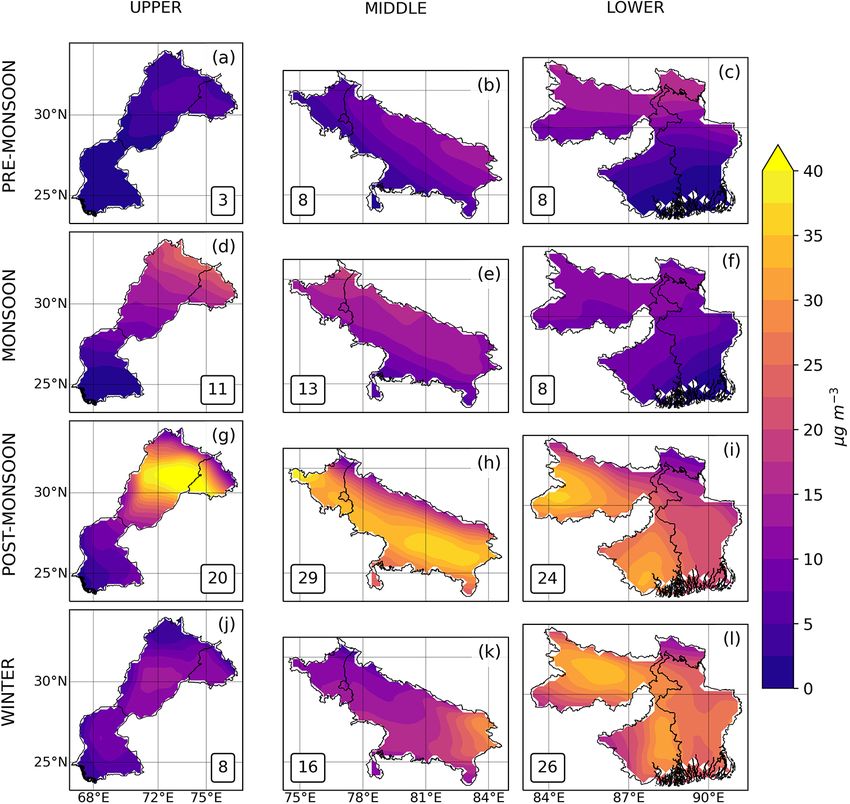
C. Mogno et al.: Fine particulate matter over the IGP                                                                       10889

Figure 3. Seasonal mean spatial distributions of PM2.5 (µg m−3 ) over the upper, middle and lower IGP. The numbers inset denote the
regional mean PM2.5 values of pre-monsoon (a–c), monsoon (d–f), post-monsoon (g–i), and winter (j–l) seasons.

best air quality is found in the Pakistani state of Sindh, with     et al., 2018). In the middle IGP, mean PM2.5 concentrations
PM2.5 concentrations below 75 µg m−3 . Biomass burning in           are 18 µg m−3 lower than post-monsoon levels, with east
the Indian Punjab plays a key role in shaping the distribu-         Delhi and Singauli remaining the largest hotspots of the re-
tion of PM2.5 during this season. Figure 4h shows that fire         gion (> 220 µg m−3 ). The upper IGP experiences the lowest
emissions have the largest impact on PM2.5 concentrations           seasonal PM2.5 concentration (86 µg m−3 ), lower than half
across the Indian and Pakistani Punjab region, Haryana, and         the value in the lower IGP, with concentrations decreasing
Delhi NCT (sensitivities of up to > 103 µg m−3 Gg−1 ). The          from the Punjab to the Sindh coast. Anthropogenic emissions
impact of post-monsoon biomass burning emissions extends            dominate the distribution of PM2.5 during winter over the
to the central part of the middle IGP over Uttar Pradesh,           lower IGP (sensitivity up to 4 × 10² µg m−3 Gg−1 , Fig. 4j),
where sensitivity of PM2.5 to pyrogenic emissions (up to            with the highest sensitivities over the cities of Kolkata and
6×10² µg m−3 Gg−1 ) is higher than anthropogenic emissions          Singrauli. The influence of biomass burning is significant
(up to 4 × 10² µg m−3 Gg−1 ).                                       over the Indus basin, stretching until Uttar Pradesh (sensi-
   The sensitivity of PM2.5 to changes in biogenic emis-            tivity up to 103 µg m−3 Gg−1 ; Fig. 4k), while biogenic emis-
sions (Fig. 4i) only has non-negligible values (< 2 ×               sions do not show a significant influence during this season
102 µg m−3 Gg−1 ) over part of West Bengal in the lower IGP.        (Fig. 4l).
   During the winter season (Fig. 3j–l), wind patterns trans-          During the pre-monsoon season (Fig. 3a–c), air quality be-
port pollutants from the upper IGP to the lower IGP, result-        gins to improve due to higher PBLHs and stronger winds
ing in a west–east gradient in seasonal mean PM2.5 con-             (Fig. A1) that help to disperse pollutants. Mean PM2.5 con-
centrations. The mean PM2.5 value in the lower IGP is               centrations are similar over the upper and middle IGP, with
191 µg m−3 , the highest mean seasonal value for the IGP.           values lower than 90 µg m−3 . Higher concentrations remain
The highest PM2.5 concentrations are reached in Kolkata (>          in the lower IGP (128 µg m−3 ) due to the accumulation of
300 µg m−3 ) and in the Bihar state, with a local peak in Patna     pollutants from the winds blowing from the Bay of Bengal
(> 220 µg m−3 ) known as the “Bihar pollution pool” (Kumar          to the slopes of the Himalayas over North Bangladesh. High

https://doi.org/10.5194/acp-21-10881-2021                                         Atmos. Chem. Phys., 21, 10881–10909, 2021
10890 C. Mogno et al.: Fine particulate matter over the IGP
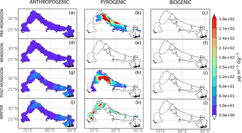
Figure 4. Seasonal sensitivity of PM2.5 concentrations to changes in (a, d, g, j) anthropogenic, (b, e, h, k) pyrogenic, and (c, f, i, l) biogenic
emissions (µg m−3 Gg−1 ). The calculation is described in the main text. Regions marked in white denote where sensitivity corresponds to
PM2.5 concentrations below the set threshold of 4 µg m−3 .
aerosol loading over the lower IGP during the pre-monsoon Surface PM2.5 composition
season is also influenced by biomass burning from North-
east India and Myanmar–Laos, which are partially included
in our model domain. PM2.5 values over the upper part of Figure 5 shows the modelled composition of PM2.5 across
the middle IGP (Fig. 3b) show some influence from biomass the IGP. Generally, we find more variability between sea-
burning (Fig. 4b). We find that anthropogenic emissions are sons than across different parts of the IGP, except for the
most important over the lower IGP and localised regions in water contribution to PM2.5 mass. The results we report
the central IGP (Fig. 4a). PM2.5 concentrations in Delhi NCT for the chemical composition and seasonal trends of PM2.5
are jointly influenced by biomass burning and anthropogenic are broadly consistent with chemical characterisation stud-
sources. Biogenic sources only have a significant impact over ies over the region (Chowdhury et al., 2007; Bhowmik et al.,
localised regions in the lower and middle IGP (Fig. 4c). 2020). As discussed in Sect. 2.3, model limitations in repro-
Generally, the onset of the monsoon results in better air ducing precursor trace gases will affect our ability to model
quality across the IGP due to higher rainfall rates, which secondary components of particulate matter. When compar-
increases wet deposition of aerosols, and higher PBLHs ing the model with recent field observations of PM1 over
that improve the physical dispersal of surface emissions. Delhi during post-monsoon and winter (Gani et al., 2019;
Mean values of PM2.5 are ≤ 100 µg m−3 across the IGP. Gunthe et al., 2021; Patel et al., 2021), corresponding to two
The largest values of PM2.5 are over the lower IGP (up to of our study seasons, we find that the model generally un-
170 µg m−3 ). We find that PM2.5 is sensitive to biogenic derestimates PM1 (57–161 µg m−3 observed, 17–22 µg m−3
emissions over localised regions across the IGP, where PM2.5 simulated), although we acknowledge that the model config-
can be more sensitive to changes in biogenic emissions than uration we use is not ideal to model submicron PM due to
changes in anthropogenic emissions (∼ 200–500 µg m−3 ) our use of four sectional size bins. The model overestimates
and < 200 µg m−3 , respectively). Fires play only a small role the contribution of PM1 from nitrate (6 %–11 % observed,
in PM2.5 during this season. 11 %–13 % simulated) but underestimates the contributions
from sulfate (7 %–9 % observed, 2 % simulated) and organ-
ics (54 %–68 % observed, 16 %–18 % simulated).
Inorganic species (secondary inorganic aerosol of sulfate,
nitrate and ammonium and other inorganic aerosol) domi-
Atmos. Chem. Phys., 21, 10881–10909, 2021 https://doi.org/10.5194/acp-21-10881-2021C. Mogno et al.: Fine particulate matter over the IGP 10891
Figure 5. Seasonal mean PM2.5 composition from the WRF-Chem model across the IGP: (a) upper, (b), middle, and (c) lower IGP. The
2−
constituents include sea salt (sum of sodium (Na) and chloride (Cl)), NH+ −
4 , SO4 , NO3 , the sum of the remaining inorganic compounds
(OTHER), total OA, BC, and liquid water.
nate the chemical composition by mass of PM2.5 , represent- The sum of primary and secondary OA contributes by
ing between 30 %–80 % of total PM2.5 for each season across mass between 17 % and 31 % of PM2.5 across the IGP,
the IGP. The mean seasonal mass of total inorganics across with contributions from POA and SOA varying with sea-
the IGP is 54–70 µg m−3 during the pre-monsoon season, son. During the pre-monsoon season, OA contributes 11–
27–35 µg m−3 during the monsoon season, 79–111 µg m−3 21 µg m−3 to PM2.5 , representing 17 %–22 % of the to-
during the post-monsoon season, and 51–114 µg m−3 dur- tal mass. A similar mass contribution is found during the
ing winter. The largest inorganic aerosol values are found monsoon season (18–21 µg m−3 ) but with higher percent-
during the post-monsoon and winter seasons due to nitrate age contribution to PM2.5 (20 %–31 %). The percentage mass
from fossil fuel combustion and from residential and energy contribution of OA to PM2.5 is similar during the post-
use. We find a similar but relatively muted seasonal variation monsoon (28 %–31 %, 43–52 µg m−3 ) and winter (22 %–
for black carbon with mass values between 2–11 µg m−3 . Sea 31 %, 26–60 µg m−3 ), with higher mass contribution during
salt transported from the coasts during the monsoon season post-monsoon for the middle and lower IGP and during the
adds 3–5 µg m−3 (3 %–9 %) to PM2.5 across the IGP. winter season for the lower IGP. Our results for modelled
The water contribution to PM2.5 is substantial over the PM2.5 composition confirm the significance of OA contribu-
lower IGP during pre-monsoon, monsoon, and post-monsoon tion to fine particulate matter, and we analyse in more detail
seasons, with a mass contribution of 32–44 µg m−3 (25 %– OA and its components in the next sections.
42 %), while during winter it accounts for 6 µg m−3 (3.5 %).
For the middle IGP, water is a non-negligible fraction of 3.3 Seasonal distribution of surface OA
PM2.5 mainly during monsoon (20 µg m−3 , 24 %) and winter
(12 µg m−3 , 8 %) seasons, while for the upper IGP the highest Figure 6 shows the season mean distributions of total OA,
values of water mass are found during only the monsoon sea- with the corresponding POA and SOA distributions shown
son (4 µg m−3 , 8 %). The seasonal variation of water content by Figs. A2 and A3. We generally find that POA dominates
reflects RH distributions, which above values of 60 %–70 % seasonal values of total OA across the IGP, with the excep-
allows PM hydrophilic components (e.g. nitrate, sulfate, sea tion of the post-monsoon season when SOA and POA have
salt) to uptake water via deliquescence. comparable values.
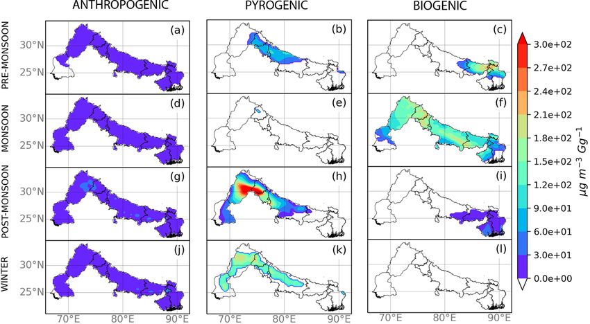
https://doi.org/10.5194/acp-21-10881-2021 Atmos. Chem. Phys., 21, 10881–10909, 202110892 C. Mogno et al.: Fine particulate matter over the IGP Figure 6. Seasonal mean distributions of total OA over the upper, middle, and lower IGP. The numbers inset denote the regional mean total OA values of pre-monsoon (a–c), monsoon (d–f), post-monsoon (g–i), and winter (j–l) seasons. During the post-monsoon season (Fig. 6g–i), the largest higher values over the Punjab to Delhi NCT and part of Uttar OA concentrations are over the upper IGP at the border of Pradesh (up to 103 µg m−3 where fires are located over Indian Pakistani and Indian Punjab (> 80 µg m−3 ), where POA val- Punjab). The sensitivity of OA to changes in biomass burn- ues can exceed 50 µg m−3 , although the largest regional mean ing is localised, with POA most influenced by fires over Pun- is found over the lower IGP (52 µg m−3 ) due to urban anthro- jab and Haryana (Fig. A4h) and the corresponding impact on pogenic emissions in and around Kolkata and Patna, where SOA extending over Pakistani Punjab and towards the mid- values are > 70 µg m−3 . Over the middle IGP, the mean OA dle IGP (Fig. A5h). Similarly, biogenic emissions play only a value is similar to the lower IGP (52 µg m−3 ) but shows a localised role in OA and SOA concentrations where biogenic more homogeneous distribution, with the highest OA values emissions are still significant during this season (Figs. 7i and found at the borders between upper and lower IGP. Regional A5i). OA is most sensitive to anthropogenic emissions over mean POA values range from 23–29 µg m−3 (Fig. A2g–i), the Indian part of the lower IGP and in the Pakistani Pun- similar to SOA values (20–24 µg m−3 ; Fig. A3g–i). POA lev- jab values (between 50–150 µg m−3 ). We find that OA over els are much higher than SOA over the Punjab states in India the Delhi NCT megacity is not sensitive to these changes un- and Pakistan and in the Indian lower IGP (40–70 and 30– like other cities mentioned previously, so that Delhi is not 40 µg m−3 for POA and SOA, respectively). Over the middle one of the main hotspots of OA across IGP during this sea- IGP, SOA is generally higher than POA (29 and 24 µg m−3 son (Fig. 6h) unlike it is for PM2.5 (Fig. 3h). We find that for SOA and POA, respectively), with highest concentrations the sensitivity of POA and SOA to changes in anthropogenic of SOA found in the lower Uttar Pradesh (up to 40 µg m−3 ). emissions is comparable across major cities of the Punjab Over Bangladesh and the Pakistani state of Sindh, POA and states (Figs. A4g, A5g). SOA have comparable values (< 35 µg m−3 ). We find that the largest seasonal mean values of OA are Similarly to PM2.5 , we find that during the post-monsoon during winter over the lower IGP (60 µg m−3 , Fig. 6j–l), season, the OA distribution across the IGP is most sensitive with contributing localised peaks over Kolkata and Patna to changes in biomass burning emissions (Fig. 7g–i), with (> 80 µg m−3 ) and at the border between Pakistan and In- Atmos. Chem. Phys., 21, 10881–10909, 2021 https://doi.org/10.5194/acp-21-10881-2021
C. Mogno et al.: Fine particulate matter over the IGP                                                                                   10893

Figure 7. Seasonal sensitivity of total OA to changes in (a, d, g, j) anthropogenic, (b, e, h, k) pyrogenic, and (c, f, i, l) biogenic emissions
(µg m−3 Gg−1 ). The sensitivity calculation is described in the main text. Regions marked in white show where sensitivity corresponds to OA
concentrations below the set threshold of 1 µg m−3 .

dia (ranging 40–70 µg m−3 ). Seasonal mean values of POA                  the monsoon season, the influence of fires on OA is negli-
and SOA also peak during winter over the lower IGP (34                    gible across the IGP. The influence of biogenic emissions on
and 26 µg m−3 , respectively.) During winter, the OA distri-              OA, determined exclusively in our model via SOA, is limited
bution is shaped by anthropogenic and pyrogenic emissions                 to the lower IGP during the pre-monsoon season. During the
(Fig. 7j–l). POA concentrations are shown to be sensitive                 monsoon season, these emissions have a widespread impact
to anthropogenic emissions in a similar way as they are for               on OA (Fig. 7f), with seasonal mean peak sensitivity of up to
the post-monsoon season (Fig. A4g, j). SOA is also mostly                 2.3 × 10² µg m−3 Gg−1 .
determined by anthropogenic emissions over the lower IGP                     PM2.5 and OA are more sensitive to changes in biogenic
(Fig. A5j). POA and SOA are also sensitive to pyrogenic                   emissions than changes in anthropogenic emissions during
emissions, but during this season it is limited to fires over             the monsoon period because of the role that anthropogenic
the Indus basin in Pakistan and central IGP (Figs. A4k, A5k).             emissions play in controlling the production of biogenic
We find that biogenic emissions do not significantly influence            SOA. Previous studies have shown that anthropogenic emis-
OA during winter.                                                         sions can enhance biogenic SOA production, with NOx con-
   During pre-monsoon and monsoon seasons, the OA distri-                 centrations playing a strong role in enhancing SOA forma-
butions (Fig. 6a–f) have similar mean values over the middle              tion from isoprene and terpenes (Spracklen et al., 2011;
and lower IGP (20–21 µg m−3 ) and lower mean values over                  Shilling et al., 2013; Shrivastava et al., 2019; Xu et al., 2020).
the upper IGP (11 and 18 µg m−3 , respectively). The high-                A disadvantage of our using a single-variable perturbative
est POA concentrations are found at the border on India and               method is that we can only consider the impacts of one con-
Pakistan and over the lower IGP (' 30 and 40 µg m−3 , re-                 trolling factor in the production of OA. Research that consid-
spectively). In both seasons, mean SOA concentrations are                 ers the interactions between controlling factors is outside the
below 15 µg m−3 across the whole IGP. During pre-monsoon                  scope of this study.
and monsoon seasons, OA concentrations are sensitive to an-
thropogenic emissions across the IGP, with similar spatial                3.4    Seasonal distribution of SOA volatility
distributions (Fig. 7a, d). Pyrogenic emissions influence the
OA distribution during the pre-monsoon season over the cen-               We use aerosol volatility to describe how SOA is partitioned
tral IGP (Fig. 7b), but OA is less sensitive to these emissions           between the gas and particle phase to understand when it
compared with the post-monsoon season (Fig. 7h). During                   contributes to PM2.5 mass loading. Figure 8 shows the sea-

https://doi.org/10.5194/acp-21-10881-2021                                                 Atmos. Chem. Phys., 21, 10881–10909, 2021
You can also read