CALC-2020: a new baseline land cover map at 10 m resolution for the circumpolar Arctic - ESSD
←
→
Page content transcription
If your browser does not render page correctly, please read the page content below
Earth Syst. Sci. Data, 15, 133–153, 2023
https://doi.org/10.5194/essd-15-133-2023
© Author(s) 2023. This work is distributed under
the Creative Commons Attribution 4.0 License.

                     CALC-2020: a new baseline land cover map
                     at 10 m resolution for the circumpolar Arctic
              Chong Liu1 , Xiaoqing Xu2 , Xuejie Feng1 , Xiao Cheng1 , Caixia Liu3 , and Huabing Huang1,2,4
          1 School of Geospatial Engineering and Science, Sun Yat-sen University, and Southern Marine Science and
                             Engineering Guangdong Laboratory (Zhuhai), Zhuhai 519082, China
                                     2 Peng Cheng Laboratory, Shenzhen 518066, China
                3 State Key Laboratory of Remote Sensing Science, Aerospace Information Research Institute,

                                    Chinese Academy of Sciences, Beijing 100101, China
           4 International Research Center of Big Data for Sustainable Development Goals, Beijing 100094, China

           Correspondence: Caixia Liu (liucx@radi.ac.cn) and Huabing Huang (huanghb55@mail.sysu.edu.cn)

                                    Received: 29 June 2022 – Discussion started: 8 August 2022
                       Revised: 15 December 2022 – Accepted: 19 December 2022 – Published: 9 January 2023

       Abstract. The entire Arctic is rapidly warming, which brings in a multitude of environmental consequences
       far beyond the northern high-latitude limits. Land cover maps offer biophysical insights into the terrestrial en-
       vironment and are therefore essential for understanding the transforming Arctic in the context of anthropogenic
       activity and climate change. Satellite remote sensing has revolutionized our ability to capture land cover in-
       formation over large areas. However, circumpolar Arctic-scale fine-resolution land cover mapping has so far
       been lacking. Here, we utilize a combination of multimode satellite observations and topographic data at 10 m
       resolution to provide a new baseline land cover product (CALC-2020) across the entire terrestrial Arctic for
       circa 2020. Accuracy assessments suggest that the CALC-2020 product exhibits satisfactory performances, with
       overall accuracies of 79.3 % and 67.3 %, respectively, at validation sample locations and field/flux tower sites.
       The derived land cover map displays reasonable agreement with pre-existing products, meanwhile depicting
       more subtle polar biome patterns. Based on the CALC-2020 dataset, we show that nearly half of the Arctic
       landmass is covered by graminoid tundra or lichen/moss. Spatially, the land cover composition exhibits regional
       dominance, reflecting the complex suite of both biotic and abiotic processes that jointly determine the Arctic
       landscape. The CALC-2020 product we developed can be used to improve Earth system modelling and benefit
       the ongoing efforts on sustainable Arctic land management by public and non-governmental sectors. The CALC-
       2020 land cover product is freely available on Science Data Bank: https://doi.org/10.57760/sciencedb.01869 (Xu
       et al., 2022a).

1   Introduction                                                   et al., 2018), vegetation greening/browning (Myers-Smith et
                                                                   al., 2020; Berner et al., 2020; Bartsch et al., 2020b) and inten-
Accounting for ∼ 5.5 % of the Earth’s land surface, the Arc-       sified greenhouse gas emissions (Najafi et al., 2015; Descals
tic disproportionately affects global biogeochemical cycles        et al., 2022). These changes have profound impacts on Arc-
(Jeong et al., 2018; Landrum and Holland, 2020; Miner et           tic biomes (Hodkinson et al., 1998; Shevtsova et al., 2020;
al., 2022) and harbours a large proportion of high-latitude        Wang and Friedl, 2019) and put millions of local residents
biodiversity (Niittynen et al., 2018; Christensen et al., 2020).   and their cultures at risk (Huntington et al., 2019). Moreover,
During the past decades, the Arctic as a whole has been            a changing Arctic is increasingly influencing human societies
rapidly warming (Previdi et al., 2021), with crucial conse-        outside of the Arctic (Moon et al., 2019), through sea level
quences for the terrestrial environment including land ice         rise and atmospheric circulation. Without effective strate-
retreat (Shepherd et al., 2020), permafrost thawing (Hjort

Published by Copernicus Publications.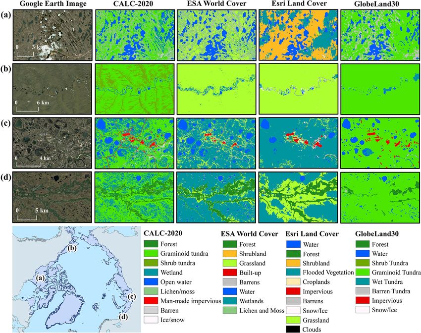
134                                                                                                     C. Liu et al.: CALC-2020

gies for mitigating Arctic environmental changes, the goal         al., 2020a). Severe cloud contamination and high solar zenith
of global sustainable development remains elusive (Beamish         angles also introduce uncertainties into the results derived
et al., 2020; C. Liu et al., 2021, 2022).                          from optical imagery (Berner et al., 2020). Hence, efforts of
   As a key terrestrial surface descriptor, land cover is cen-     mapping circumpolar Arctic land cover should be comple-
tral to our understanding of the changing Arctic (Bartsch et       mented by information beyond the spectral domain. Space-
al., 2016; Liang et al., 2019; Raynolds et al., 2019; Wang         borne synthetic aperture radar (SAR) is capable of penetrat-
et al., 2020). The land cover regulates the surface energy         ing clouds and thus providing valuable Earth observation in-
fluxes, which contribute to climate change and, in turn, in-       formation when and where valid optical image data are in-
fluence land surface properties and the provision of ecosys-       sufficient (Engram et al., 2013). Recent studies have sug-
tem services (Friedl et al., 2010; Gong et al., 2013; Wulder       gested that the inclusion of SAR data is essential for generat-
et al., 2018; Song et al., 2018). Given the Arctic’s ecologi-      ing spatially continuous maps of land cover within the Arctic
cal importance, some earlier efforts were made to map Arc-         (Bartsch et al., 2020a, 2021). In addition to optical and SAR
tic land cover based on field investigations (Ingeman-Nielsen      data, terrain coefficients can also facilitate the identification
and Vakulenko, 2018; Lu et al., 2018) or existing atlases          of Arctic biomes by incorporating environmental factors in-
(Walker et al., 2005; Raynolds et al., 2014), both of which        cluding temperature, solar radiation and water availability
are nevertheless laborious, time-consuming and resource-           (Raynolds et al., 2019). Furthermore, the rapid development
demanding. With a synoptic view and repeatable coverage,           of cloud computing platforms, such as Google Earth Engine
satellite observations provide an unprecedented way to delin-      (GEE) (Gorelick et al., 2017), Amazon Web Services (AWS)
eate and analyse Arctic land cover at multiple scales. A few       (H. Liu et al., 2021) and NASA Earth Exchange (NEE) (Ne-
studies attempted to capture Arctic land cover using satel-        mani et al., 2010), enables full advantage to be taken of geo-
lite remote sensing, with observations obtained from satel-        big data, thus making multi-source-based circumpolar Arctic
lites of Landsat (Jin et al., 2017; Wang et al., 2020), SPOT       land cover mapping feasible.
(Kumpula et al., 2011) and Sentinel-2 (Bartsch et al., 2020a).        In this study, we present a new circumpolar Arctic
But these studies focused mainly on small areas, being un-         land cover product for circa 2020 (CALC-2020 hereafter),
able to provide spatially complete information for the en-         through synergistically integrating multimode remote sens-
tire terrestrial Arctic. In parallel, some existing scientific     ing data captured by the Sentinel satellite sensors and ter-
programmes have manifested remarkable achievements of              rain layers derived from the recently released ArcticDEM.
general-purpose land cover maps at the global scale, includ-       Within the Arctic extent, each land pixel is characterized
ing (part of) the Arctic region (Loveland et al., 2000; Friedl     by its dominant biophysical component using a modified
et al., 2010). However, these products have coarse spatial res-    FROM-GLC (Finer Resolution Observation and Monitoring
olutions (100 m–1 km pixel size), hence raising the sub-pixel      of Global Land Cover) classification scheme, at 10 m spa-
mixing issue (Friedl et al., 2022). Recent advances in satellite   tial resolution. To create the CALC-2020 map, metrics were
data accessibility offer a new possibility to explore large-area   derived from Sentinel-1 polarization, Sentinel-2 surface re-
environmental change (Gong et al., 2013). Different from           flectance and ArcticDEM topographic bands, serving as in-
traditional products derived from coarse-resolution imagery,       put features for a machine-learning classification procedure
fine-resolution (10–30 m pixel size) land cover datasets are       based on the GEE platform. The classification model was
now becoming available at continental to global scales.            locally calibrated with a training sample set collected from
   Although the entire Earth surface has witnessed a growing       multiple data sources. We aim, by resolving the most updated
number of fine spatial resolution land cover products (Gong        spatial patterns and composition of land cover across the ter-
et al., 2013; Chen et al., 2015; Karra et al., 2021; Zanaga et     restrial Arctic, to advance our knowledge of environmental
al., 2021; Brown et al., 2022), most of them have systemat-        change at northern high latitudes and to enlighten sustainable
ically low accuracy in Arctic (Bartsch et al., 2016; Liang et      land management by public and non-governmental sectors.
al., 2019), thus not fully meeting the need for precise Arc-
tic land cover distribution and composition information. The
                                                                   2     Materials and methods
terrestrial Arctic environment is a fundamentally different
ecosystem from lower latitudes, and this calls for reconsider-     2.1    Study area and land cover classification scheme
ation of land cover mapping paradigm from aspects includ-
ing classification legend design, remote sensing data acquisi-     There exist various definitions of what extent is contained
tion and computing performance. For example, the lichen/-          within the Arctic. In the present study, we delimited the study
moss biome is extensively distributed within high-latitude         area in the terrestrial Arctic, following our previous prac-
ecozones, but such a type is absent in most land cover classi-     tices by C. Liu et al. (2021) and Xu et al. (2022b). Here the
fication schemes (Friedl et al., 2022). Moreover, the common       terrestrial Arctic is defined as the northernmost part of the
presence of treeless tundra landscape patches gives rise to the    Earth characterized by tundra vegetation, an arctic climate
“spectral confusion” issue that can lead to a decreased classi-    and arctic flora, with the tree line and continental coastlines
fication accuracy in the Arctic (Liang et al., 2019; Bartsch et    jointly determining the extent borders (Fig. 1). Spatially,

Earth Syst. Sci. Data, 15, 133–153, 2023                                             https://doi.org/10.5194/essd-15-133-2023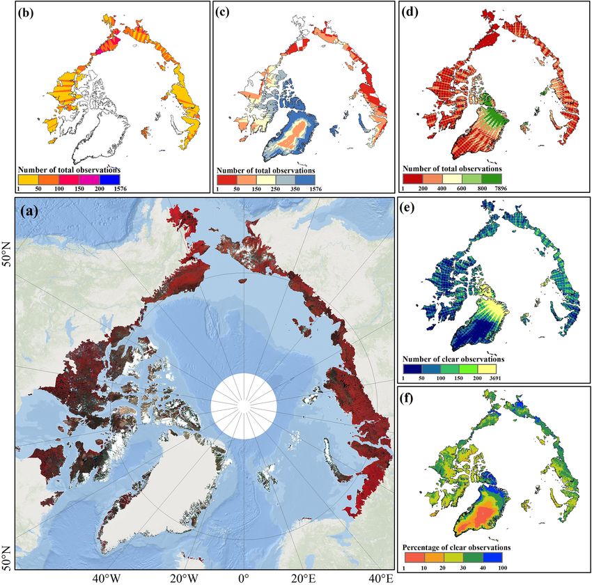
C. Liu et al.: CALC-2020                                                                                                     135

the present study covers an area of approximately 7.11 ×         2.3     Creation of CALC-2020 map
106 km2 , overlapping with parts of six countries including
Canada (CA), Denmark (Greenland, GR), Iceland (IC), Nor-         Based on input data from Sentinel-1, Sentinel-2 and Arctic-
way (NO), Russia (RU) and the United States (Alaska, AK).        DEM, we developed a comprehensive framework (Fig. 2) to
Within the study area, we implemented a 10-category classi-      guide circumpolar Arctic land cover mapping and analysis
fication scheme to represent the land cover diversity across     at 10 m spatial resolution for circa 2020. For the purpose of
the terrestrial Arctic. This scheme evolved from the level-1     supervised classification model development, a “ready-for-
classification system of FROM-GLC version 2017 (Gong et          use” training sample set was constructed derived from multi-
al., 2019), with necessary modifications that adapt to the ge-   ple sources. We created two separate circumpolar Arctic map
ographical environment at northern high latitudes (Liang et      products: a map of the man-made impervious surface extent
al., 2019). More specifically, we excluded the grassland class   and a map of the natural land cover distribution. For map-
due to its rareness and subdivided the tundra biome into three   ping the man-made impervious surface extent, we directly
categories: graminoid tundra, shrub tundra and lichen/moss.      leveraged the existing circumpolar Arctic Man-made imper-
Table 1 provides the definition of each land cover type in-      vious area product (CAMI-2020) from our pilot study (Xu
cluded in the present study.                                     et al., 2022b). For mapping the natural land cover distribu-
                                                                 tion, we developed local adaptive random forest models for
                                                                 each country and performed supervised classification using
2.2   CALC-2020 input data
                                                                 polarimetric, spectral, phenological and topographic feature
We used the GEE platform to obtain and preprocess remote         metrics. Detailed procedures within the framework are de-
sensing datasets in this study. All image collections were       scribed below.
independently filtered by the extent of the study area and
the study period (the year 2020). The Sentinel-1 mission is
                                                                 2.3.1    Training sample set construction
composed of a constellation of two satellites (S-1A and S-
1B), both performing dual-polarization C-band SAR imag-          The supervised land cover classification approach requires
ing with a 12 d repeat cycle at the Equator. Among vari-         reliable training sample for model development (Foody et
ous Sentinel-1 products, we used the Level 1 Ground Range        al., 2016; Hermosilla et al., 2022). In the present study,
Detected (GRD) product in the interferometric wide (IW)          the CALC-2020 training sample set was constructed from
swath mode at 10 m spatial resolution. Given the imbalanced      three sources (Fig. S1). First, we used the world’s first all-
data coverage of polarization combinations across the Arc-       season sample library (FAST) (Li et al., 2017) to generate
tic (Fig. 1b and c), we selected dual-band cross-polarization,   the backbone of our training data. FAST offers 91 619 sam-
horizontal transmit/vertical receive bands (HH + HV) for         ple locations and their multi-seasonal land cover type infor-
Canada and Greenland and the dual-band cross-polarization,       mation at the planetary scale for circa 2017. We excluded
vertical transmit/horizontal receive bands (VV + VH) for the     FAST records that are outside of our study area or expe-
remaining countries. The Sentinel-2 Multi-Spectral Instru-       rienced land cover change(s) by conducting spectral simi-
ment (MSI) on board both S-2A and S-2B satellites is an          larity measurement between the reference year (i.e. 2017)
optical sensor which started observing the Earth’s terres-       and the target year (i.e. 2020) (Huang et al., 2020). For
trial surface in 2015, with a spatial resolution of 10–60 m      each retained FAST sample location, we created a 90 × 90 m
depending on the wavelength. The present study used the          square buffer in which the land cover labels of all pixels
Level 2 surface reflectance product of Sentinel-2 to ensure      were acquired by leveraging the SCL band layer of Sentinel-
that geometric and radiometric qualities meet the require-       2 (C. Liu et al., 2021). A FAST sample record was pre-
ments. For each Sentinel-2 image, three visible bands, four      served only when it represented the dominant land cover type
red edge bands, three infrared bands, one scene classification   within its buffer area (i.e. greater than 50 % area proportion).
map band (SCL) and one quality assessment band (QA60)            The above-mentioned procedure resulted in a total of 14 579
were employed. We pan-sharpened the red edge and infrared        preliminary sample records derived from FAST. The second
bands to 10 m using the bicubic interpolation algorithm (Liu     source of training data is existing land cover maps, including
et al., 2020) to match the resolution of visible bands. In ad-   NLCD 2016 (for Alaska), Land Cover of Canada 2015 (for
dition to satellite imagery, we also included the 10 m Arc-      the Canadian Arctic) and GlobeLand30 V2020 (for the re-
ticDEM digital surface model product in our data pool for        maining terrestrial Arctic countries). We incorporated these
characterizing the topographic properties of each Arctic land    products into one single land cover mapping layer by unify-
pixel. Encompassing all land area north of 60◦ N, the Arctic-    ing their classification schemes into the CALC-2020 legend
DEM v3.0 product was generated from very high-resolution         (Table 1) based on prior knowledge. For example, wet tun-
(VHR) stereo images (Porter et al., 2018).                       dra (GlobeLand30) and grassland/herbaceous (NLCD 2016)
                                                                 land cover types are equivalent to wetland and graminoid tun-
                                                                 dra, respectively, due to their similar definitions. With the re-
                                                                 classified reference land cover layer, sample extraction was

https://doi.org/10.5194/essd-15-133-2023                                           Earth Syst. Sci. Data, 15, 133–153, 2023
136                                                                                                              C. Liu et al.: CALC-2020

Figure 1. Overview of the study area. (a) Spatial extent of the circumpolar Arctic, located at the northernmost part of the Earth with a total
area of ∼ 7.11 × 10⁶ km2 . Bands 8, 4 and 3 are displayed as red, green and blue layers for the Sentinel-2 composite image. The base map
is from ESRI. Panels (b) and (c) show spatial distributions of per-pixel satellite observation availability for Sentinel-1 with VV + VH and
HH + HV band combinations, respectively. Panels (d), (e) and (f) are spatial distributions of total observations, clear observations and clear
observation percentage of Sentinel-2.

performed using a stratified random sampling strategy. We                graminoid tundra and shrub tundra because they are easily
randomly collected 12 000 points for each CALC-2020 class,               confused for a single season. Thus, time series images from
except for cropland (200 points), forest (2000 points) and               Sentinel-1 and Sentinel-2 were used to support judgement as
shrub tundra (5000 points) because of their limited area oc-             needed. After removing pixels deemed incorrect, we retained
cupations. All extracted points were double-checked by se-               64 133 preliminary training sample points derived from ex-
nior interpreters to minimize errors associated with the data            isting land cover maps. Given the absence of the lichen/-
source. Special care was taken to make a distinction between             moss class in FAST and most existing land cover prod-

Earth Syst. Sci. Data, 15, 133–153, 2023                                                    https://doi.org/10.5194/essd-15-133-2023
C. Liu et al.: CALC-2020                                                                                                          137

Table 1. Description of the 10-category land cover classification scheme used in the present study.

                     Land cover type (ID)              Description
                     Cropland (CRO)                    Arable land that is sowed or planted at least once within a 12-
                                                       month period, including irrigated or rain-fed field, plantation
                                                       and greenhouse
                     Forest (FST)                      Land covered by trees, with canopy coverage greater than 30 %
                                                       and canopy height typically no less than 2 m
                     Graminoid tundra (GRT)            Land covered by herbaceous vegetation with plant height typi-
                                                       cally ranging 5–15 cm
                     Shrub tundra (SRT)                Land covered by shrubs of any stature with plant height typi-
                                                       cally ranging 20–50 cm
                     Wetland (WET)                     Land featured by aquatic plants and periodically saturated with
                                                       or covered by water
                     Open water (OWT)                  Inland open water bodies, including rivers, lakes, reservoirs, pits
                                                       and ponds
                     Lichen/moss (LAM)                 Bedrock covered by cryptogam communities
                     Man-made impervious (MMI)         Impermeable land surface paved by man-made structures
                     Barren (BAR)                      Natural dry land with vegetation coverage typically less than
                                                       10 %
                     Ice/snow (IAS)                    Land covered with snow and ice all year round

Figure 2. Framework of creating CALC-2020 map with the use of Sentinel-1, Sentinel-2 and ArcticDEM data.

https://doi.org/10.5194/essd-15-133-2023                                                      Earth Syst. Sci. Data, 15, 133–153, 2023
138                                                                                                   C. Liu et al.: CALC-2020

ucts, we additionally adopted Google Earth imagery data and       features, and it provides the first spatially continuous map
UAV aerial images provided by the United States Geolog-           of Arctic man-made impervious surface distribution at 10 m
ical Survey (USGS) as the source of lichen/moss training          resolution. Accuracy assessment suggested that the CAMI-
sample. Spatial/contextual information domains of reference       2020 map is capable of depicting the spatial pattern of man-
VHR images were used to discriminate lichen/moss from             made impervious surfaces across the Arctic, with overall
other vegetated covers. The sample size of lichen/moss was        accuracy and kappa value of 86.4 % and 0.7, respectively.
5000 to balance sampling representativeness and interpre-         Due to its robustness, CAMI-2020 was used for mapping the
tation workload. We kept only well-interpreted points with        Arctic man-made impervious surface extent in the present
high-level confidence, which eventually led to 4913 prelimi-      study. The CAMI-2020 dataset is publicly available from
nary training sample points for lichen/moss.                      https://doi.org/10.11922/sciencedb.01435 (Xu et al., 2022c).
   Due to inherent classification scheme inconsistence and
acquisition year mismatch among multiple sources, the pre-        2.3.3   Natural land surface mapping
liminary training sample inevitably contains errors that could
undermine or even lead to the failure of CALC-2020 map-           After acquiring the extent of man-made impervious surface,
ping. Therefore, we conducted a refinement approach to ob-        we conducted natural surface land cover mapping based on
tain a ready-for-use training sample set based on the self-       feature metrics derived from Sentinel-1, Sentinel-2 and Arc-
organizing map (SOM) technique. The SOM, also known as            ticDEM. For Sentinel-1, a seasonal compositing approach
the Kohonen neural network, is an effective and automatic         was undertaken to obtain the median value of all obser-
tool for the task of clustering and classification (Kohonen,      vations for growing months (June, July and August) and
2013). It represents the input data distribution using a two-     dormant months, separately. For Sentinel-2, we first iden-
dimensional map in which models are automatically asso-           tified and masked invalid observations, including clouds,
ciated with neurons. In this study, we created and trained        cloud shadows and snow, according to the QA60 band. Then
a 10 × 10 map of 100 neurons using the batch weight/bias          three groups of Sentinel-2 feature metrics were extracted:
training algorithm. The map training is complete when the         (1) per-band values representing growing season reflectance
maximum number of epochs is reached (i = 200). Figure 3           using median and greenest compositing methods, respec-
illustrates the procedure of SOM-based sample refinement.         tively; (2) per-index values representing selected percentiles
For a given land cover class C (other land cover classes          (10 %, 50 % and 90 %); and (3) phenometrics including the
termed Rs), we randomly selected N sample records labelled        start of the growing season (SOS), the end of the grow-
as C and 2N sample records labelled as Rs from the pre-           ing season (EOS), the peak of the growing season (POS)
liminary training sample, respectively. We then grouped the       and the largest data value of the growing season (LDOG).
selected sample into 100 clusters, within each of which the       To reduce the impact of noise and data gaps in Sentinel-2
purity index was acquired by calculating the percentage of        time series, we followed a statistic-based algorithm (Bolton
sample records labelled as C. We set a purity index thresh-       et al., 2020) to estimate the phenometrics (Fig. S2). Cloud-
old of 75 %, aiming to balance sample size and sample ro-         free Sentinel-2 observations were interpolated in each pixel
bustness (Gong et al., 2019). This approach was applied to        at an 8 d time step using penalized cubic smoothing splines.
all classes for constituting the ready-for-use training sample.   With the smoothed, seamless reflectance time series, we cal-
After the SOM-based refinement, the final training sample         culated the normalized difference vegetation index (NDVI) at
includes 70 260 valid records, including 192, 2836, 15 686,       each temporal interval to depict the time (day of year; DOY
4794, 6470, 11 729, 4380, 11 445 and 12 728 points for crop-      hereafter) of the vegetation phenophase transitions. The max-
land, forest, graminoid tundra, shrub tundra, wetland, open       imum value of the smoothed NDVI time series was identi-
water, lichen/moss, barren and ice/snow, respectively.            fied as LDOG. SOS and EOS were retrieved as the DOYs
                                                                  when the NDVI time series crossed 50 % of the amplitude in
2.3.2   Man-made impervious surface mapping
                                                                  the green-up and green-down periods, respectively. POS was
                                                                  identified as the DOY when the NDVI time series reached
The man-made impervious surface is a representative land          LDOG. Topographic metrics were directly computed from
cover type indicating the human footprint. However, map-          ArcticDEM, including elevation, slope and aspect. In sum-
ping man-made impervious surfaces has been difficult be-          mary, we created a total of 51 feature metrics for natural land
cause they consist of diverse artificial materials and spatial    surface classification. Table S1 provides detailed descriptions
forms (Liu et al., 2022). This issue becomes more prominent       of the metrics used in the present study.
in the Arctic where impervious surface clusters are usually           Based on all metric sets described above, we used the
fragmented and small in size (e.g. oil/gas deposits). There-      random forest classifier (RFC) to generate Arctic’s natural
fore, we leveraged an existing product, CAMI-2020, from           land cover map. RFC is a non-parametric machine-learning
our pilot study (Xu et al., 2022b) to pre-classify Arctic man-    method that creates an ensemble of a multitude of deci-
made impervious surfaces. CAMI-2020 was developed by              sion trees for class membership prediction (Breiman, 2001).
integrating satellite imagery and OpenStreetMap as input          Compared with other supervised classification algorithms,

Earth Syst. Sci. Data, 15, 133–153, 2023                                           https://doi.org/10.5194/essd-15-133-2023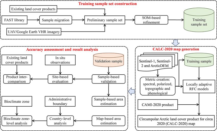
C. Liu et al.: CALC-2020                                                                                                           139

Figure 3. Illustration of the SOM-based training sample refinement procedure.

RFC is more robust in mapping large-area land cover and               site, the dominant land cover type was determined by refer-
can accommodate high dimension input features (Zhu et al.,            ring to its metadata as well as the near-surface camera images
2012; Gong et al., 2020b; X. Zhang et al., 2021). For the             (if available). The third evaluation method is the comparison
purpose of balancing classification accuracy and computa-             of CALC-2020 with three widely used global fine-resolution
tional efficiency, we parameterized RFC with 500 decision             land cover products: ESA WorldCover V100 (Zanaga et al.,
trees and the square root of the total number of input vari-          2021), ESRI Global Land Cover (Karra et al., 2021) and Glo-
ables as the number of variables to split each node (Liu et al.,      beLand30 V2020 (Chen et al., 2015). These products were
2019). RFC model training and prediction were performed               selected because (1) they have consistent data epochs and ad-
individually for each country using the “smileRandomFor-              equate spatial resolutions that make them comparable to the
est” API in GEE.                                                      CALC-2020 map and (2) they include the majority of land
                                                                      cover types used in CALC-2020 legend; thus the comparing
                                                                      results can be more robust and less affected by the classi-
2.4   Mapping performance evaluation
                                                                      fication scheme discrepancy. It should be noted that neither
We designed three methods to evaluate the performance of              selected land cover products nor CALC-2020 is considered
CALC-2020. First, we implemented a stratified random sam-             ground truth. Instead, the inter-comparison provides an over-
pling (Fig. S3) for assessing the accuracy and uncertainty            all insight of pixel-level agreement, both statistically and spa-
of our estimated land cover map, based on good practices              tially (Liu et al., 2020). At the per-pixel level, the paired land
by Olofsson et al. (2014). We used the CALC-2020 map it-              cover comparison result consists of four categories: agree-
self as the stratification of study area and set the validation       ment (AG), disagreement due to model prediction (DM), dis-
sample size to 6513 by specifying a target standard error             agreement due to scheme difference (DS) and disagreement
for overall accuracy (OA) of 0.5 %. We allocated 40–1872              due to data missing (DD). Table 2 offers the detailed defini-
sample units for each land cover class (see Sect. 3.1.1) and          tion of each paired land cover comparison category. As an
calculated error metrics including the user’s and producer’s          additional comparison to complement the inter-product eval-
accuracies (UA and PA), along with estimates of associated            uation, we used the validation sample shown in Fig. S3 to
95 % confidence intervals. The reference class label for each         calculate accuracy metrics of three global land cover prod-
sampled pixel was identified based on expert interpretation           ucts. To harmonize various classification legends to the leg-
of cloud-free Sentinel-2 images and Google Earth VHR im-              end of CALC-2020, the grass (ESA WorldCover and ESRI
agery data, as available. Sample pixels with disagreement             Global Land Cover) and wet tundra classes (GlobeLand30)
among experts were subsequently revisited until a consen-             were treated as equivalents of graminoid tundra and wetland,
sus was reached. In the second evaluation method, we exam-            respectively.
ined the CALC-2020 mapping performance using in situ data
obtained from ORNL DAAC’s MODIS/VIIRS Land Prod-                      2.5   Land cover area estimation
uct Subsets project (ORNL DAAC, 2017). We employed the
Fixed Sites Subsets Tool to select all field and flux tower sites     We performed land cover area estimation at two stages to
within our study area (55 sites in total; Table S2). For each         ensure the validity of all statistics reported throughout this

https://doi.org/10.5194/essd-15-133-2023                                                Earth Syst. Sci. Data, 15, 133–153, 2023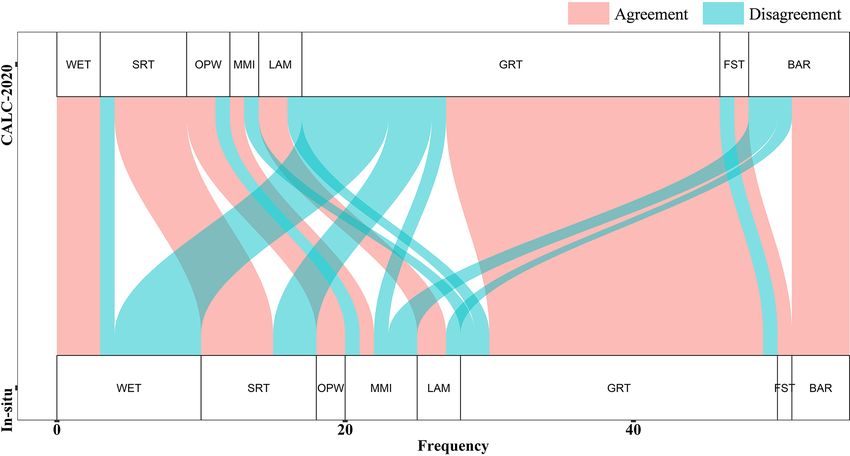
140                                                                                                         C. Liu et al.: CALC-2020

Table 2. Description of per-pixel level comparison categories between CALC-2020 and reference products.

              Category (abbreviation)                      Definition
              Agreement (AG)                               CALC-2020 and the compared land cover product display iden-
                                                           tical classification result
              Disagreement due to model prediction (DM)    CALC-2020 and the compared land cover product display dif-
                                                           ferent classification results, both of which are included in the
                                                           CALC-2020 map legend
              Disagreement due to scheme difference (DS)   The compared land cover product displays a classification result
                                                           which is not included in the CALC-2020 map legend
              Disagreement due to data missing (DD)        Unclassified or data missing exhibited by the compared land
                                                           cover product

study. At the first stage, we utilized the error matrix ob-             proportion; therefore they are inevitably different from those
tained from validation to produce “unbiased” circumpolar                derived from a traditional confusion matrix of sample counts.
Arctic land cover area estimations as well as their uncertain-          For example, the traditional confusion matrix-derived PA of
ties (95 % confidence interval). For each CALC-2020 class,              shrub tundra is 68.1 % (Table S3), whereas its stratified error-
the area estimator is based on the mapping stratum, the pro-            adjusted PA estimate is lower, due primarily to the influ-
portion estimated from the reference data and its standard              ence of estimation weights (area proportions of map classes).
error (Olofsson et al., 2014). Despite the potential of cor-            Given the generally large reflectance discrepancy between
recting area estimation biases, the sample-based area estima-           water and non-water covers, the less desirable performance
tion strategy is highly dependent on sample allocation, which           of CALC-2020 in water extraction may seem unexpected.
may unnecessarily limit its effectiveness in the Arctic be-             This highlights the distinctiveness of Arctic’s geographical
cause of the highly imbalanced sample availability among                environment that can affect the spectral signal of water in
countries and across bioclimate zones (Liu et al., 2022).               space and time (Gong et al., 2016). Specifically, shallow wa-
Therefore, at the second stage, we employed the conventional            ter bodies are easily confused with barren lands because of
pixel counting method (Gong et al., 2020b) to calculate area            the mixed pixel issue (Fig. S4a and b). Moreover, the em-
statistics directly from the CALC-2020 dataset. This map-               ployed satellite images may only capture the freezing stage
based area estimation strategy is straightforward and flexi-            for some water pixels, which were misclassified as ice/snow
ble at different spatial levels. We treated sample-based and            in the CALC-2020 map (Fig. S4c).
map-based area statistics as complementary metrics for bet-                To further evaluate the CALC-2020 mapping perfor-
ter describing the CALC-2020-derived land cover patterns at             mance over space, we divided the entire study area into
multiple levels.                                                        50 km × 50 km grids. Then the classification confidence in
                                                                        each grid was computed as the proportion of correctly clas-
                                                                        sified validation sample points (Fig. 4). Overall, we esti-
3     Results and discussion
                                                                        mated that the CALC-2020 classification confidence is 0.795
3.1     Reliability of CALC-2020 map                                    (±0.323, 1 standard deviation). Among 2037 grids that have
                                                                        at least one validation sample record, 1406 (60.9 %) show
3.1.1    Sample-based evaluation                                        confidence levels higher than 0.75. Theses grids are repre-
                                                                        sentative over space, by country and by continent. The dom-
Following good practices by Olofsson et al. (2014), we built
                                                                        inance of high-confidence grids mirrors small percentages
the error matrix and associated sample-based accuracy statis-
                                                                        held by those having low-confidence levels (less than 0.25).
tics of the CALC-2020 map based on 6513 validation points
                                                                        Spatially, hotspots of large classification uncertainty were
(Table 3). The OA of the CALC-2020 dataset for the cir-
                                                                        commonly detected in regions with a sparse validation sam-
cumpolar Arctic is 79.3 ± 1.0 % (95 % confidence interval).
                                                                        ple distribution (Fig. S3), such as the Greenland periphery,
At the biome level, we found the classifications of all land
                                                                        central Siberia and the American Arctic Archipelago.
cover types have reasonable accuracies, with UA ranging
from 74.0±2.7 % (ice/snow) to 95.9±5.6 % (man-made im-
pervious). Similarly, most biomes exhibit satisfactory PA re-           3.1.2   Land cover mapping performance in field and flux
sults (above 75 %), except for shrub tundra (47.1 ± 5.7 %),                     tower sites
open water (62.7 ± 2.7 %) and barren (62.2 ± 5.9 %) biomes
with less desirable results. It should be noted that all met-           Figure 5 displays the alluvial diagram of performance eval-
rics reported in Table 3 are based on an error matrix of area           uation for the CALC-2020 product in field and flux tower

Earth Syst. Sci. Data, 15, 133–153, 2023                                                 https://doi.org/10.5194/essd-15-133-2023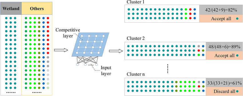
C. Liu et al.: CALC-2020                                                                                                                 141

Table 3. Error matrix of the CALC-2020 map based on the validation sample. UA, PA and OA indicate the user’s accuracy, producer’s
accuracy and overall accuracy, respectively. Reference classes are in columns. Land cover abbreviations are given in Table 1. Bold font
denotes correctly classified sample points.

  Class           CRO           FST          GRT          SRT         WET         OWT         LAM          MMI           BAR           IAS
  CRO                43             0            3            0            0          0            0            0            0            0
  FST                 0            30            2            8            0          0            0            0            0            0
  GRT                 0             0        1501            62           81         28         125             0           35            0
  SRT                 0             0           25         160             1          0            2            0            1            0
  WET                 0             0           35            5         375          14           30            0            4            0
  OWT                 0             0            2            0            0       458             0            0           17           12
  LAM                 0             0           22            0           10          1        1145             0         272            40
  MMI                 0             0            1            0            0          0            0           47            0            1
  BAR                 0             0            0            0            4         42         154             0         687            28
  IAS                 0             0            0            0            0       176            10            0           74         740
  UA (%)     93.5 ± 7.2   75.0 ± 13.6   81.9 ± 1.8   84.7 ± 5.1   81.0 ± 3.6 93.7 ± 2.2   76.8 ± 2.1   95.9 ± 5.6   75.1 ± 2.8   74.0 ± 2.7
  PA (%)           100            100   95.1 ± 1.0   47.1 ± 5.7   82.0 ± 2.9 62.7 ± 2.7   78.3 ± 2.0         100    62.2 ± 5.9   90.4 ± 1.9
  OA (%)                                                                79.3 ± 1.0

sites. Overall, our estimation is reasonably consistent with             classification agreements (area proportion of AG) range from
the in situ reports and outperforms three widely used global             23.1 % (ESRI Global Land Cover) to 45.4 % (GlobeLand30)
land cover products (Fig. S5). There are 37 out of 55 sites              by treating our estimates as the baseline. Spatially, large AG
showing consistent classification results, with an OA value              variations were also detected across biomes and among coun-
equal to 67.3 %. When the analysis is broken down into the               tries. The mapped disagreements were induced by multiple
biome level, the biggest error source comes from confusion               factors. First and foremost, the CALC-2020 classification
among different vegetation types. In particular, there are six           scheme is different from the schemes of compared land cover
wetland sites and three shrubland tundra sites that were mis-            products. This leads to considerable pixels being identified
takenly identified as graminoid tundra. These discrepancies              as DS, especially for ESA WorldCover (29.7 %) and ESRI
reflect the complex suite of factors that can obscure the cor-           Global Land Cover (56.5 %) in which the graminoid tundra
rect identification of Arctic biomes. For example, some wet-             class is absent. Another issue that can cause the inconsis-
land vegetation species are morphologically similar to grami-            tency is the difference of classification model prediction. For
neous plants, thus limiting the classification accuracy (Mag-            example, in the Canadian Arctic, a latitudinal north (high)–
nússon et al., 2021). The relatively poor mapping perfor-                south (low) contrast in land cover mapping agreement is ev-
mance of Arctic vegetation could also be attributed to the               ident when comparing our map to the GlobeLand30 dataset.
short growing season (typically ranging from 50 to 60 d),                Such a discrepancy is primarily due to the misclassification
in which satellite coverage is commonly spatially and tem-               of lichen/moss as graminoid tundra by GlobeLand30. Con-
porally uneven (Beamish et al., 2020). Considerable mis-                 sistently across all countries, DD plays a minor role with
classifications were also observed in some sites dominated               very limited area occupation (less than 5 %). Using the same
by man-made impervious surfaces, suggesting the technical                sample-based evaluation approach applied to CALC-2020,
challenge of capturing small-scale artificial imperviousness             we reported limited classification accuracies of three global
using the CALC-2020 map. It is important to point out that               land cover products for the circumpolar Arctic (Fig. 7), with
the field and flux tower sites used in the present work are              OAs ranging from 48.5 % to 71.2 %. In the meantime, these
not evenly distributed over space and across biomes. Some                global-scale datasets exhibit wide PA and UA variations, im-
land cover types (e.g. forest and lichen/moss) have very lim-            plying imbalanced mapping performances across different
ited sites after data screening, making them less representa-            Arctic land cover types (Liang et al., 2019).
tive for mapping performance evaluation. This situation will                Figure 8 further compares multiple land cover datasets by
be improved as more ground and near-surface reference data               selecting four subregions, each of which represents one typi-
become available in the future (Richardson et al., 2018; Pas-            cal landscape across the terrestrial Arctic. The Google Earth
torello et al., 2020).                                                   image of each subregion is also displayed for assisting map-
                                                                         ping performance evaluation. All land cover products are dis-
                                                                         played with their corresponding classification schemes. In
3.1.3     Comparison with existing land cover products                   Keewatin (Canada), all the products correctly capture most
                                                                         open water areas. Compared to other land cover datasets, the
Figure 6 displays the spatial patterns and statistics of agree-          CALC-2020 map is more similar to GlobeLand30 in terms
ment/discrepancy between the CALC-2020 map and three                     of the overall land cover composition and distribution. In
global land cover products. At the circumpolar Arctic scale,

https://doi.org/10.5194/essd-15-133-2023                                                    Earth Syst. Sci. Data, 15, 133–153, 2023
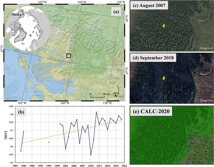
142                                                                                                          C. Liu et al.: CALC-2020

Figure 4. Map of CALC-2020 classification confidence calculated at a 50 km × 50 km tile scale. The grey grid denotes no validation sample
point distribution. The bar plot shows the statistical distribution of six broad classification confidence intervals.

North Slope (Alaska), our estimation detects the coexistence           ESRI Global Land Cover, on the other hand, show greater
of graminoid tundra and shrub tundra, with their distributions         wetland estimates. Moreover, CALC-2020 is the only land
highly related to topographic characteristics. This heteroge-          cover product that fully depicts the distribution of man-made
nous land cover pattern, however, is not observed in the other         impervious surfaces (oil/gas deposits and traffic pavements).
three products. The reasonable performance of the CALC-                In Nenets, major forest clusters are correctly identified by
2020 map for North America was also confirmed by refer-                the three datasets with a finer resolution of 10 m, includ-
ring to two national-scale land cover products: NLCD and               ing CALC-2020, ESA WorldCover and ESRI Global Land
Land Cover of Canada, both of which exhibit a high agree-              Cover. However, the latter two products are not able to isolate
ment of the land cover distribution pattern with CALC-2020             graminoid plants from wetlands, both of which are clearly
in their level-1 classification schemes (Fig. S6). For the Rus-        displayed by our mapping result. In summary, our estima-
sian Arctic, the largest mapping discrepancy among different           tions capture more subtle polar biome patterns than three
mapping results is found in Yamal Peninsula, where more                global land cover products, although they were generated to
than half of the landmass is covered by thermokarst lakes.             depict general-purpose land cover at global scales.
Our dataset is generally consistent with GlobeLand30 but
provides many more spatial details. ESA WorldCover and

Earth Syst. Sci. Data, 15, 133–153, 2023                                                 https://doi.org/10.5194/essd-15-133-2023
C. Liu et al.: CALC-2020                                                                                                             143

Figure 5. CALC-2020 map performance in 55 field and flux tower sites. The block width represents the frequency (site number) identified
by our estimation and in situ reports, respectively. Land cover abbreviations are given in Table 1.

3.2   Spatial patterns and composition of circumpolar                     is the result of persistent disturbances from industrial infras-
      Arctic land cover                                                   tructure development and traffic pavements (Bartsch et al.,
                                                                          2021; Xu et al., 2022b).
The CALC-2020 product provides the first spatially contin-                   By disaggregating land cover composition at multiple
uous map of circumpolar Arctic land cover at 10 m resolu-                 scales, the CALC-2020 map offers mechanistic insights into
tion (Fig. 9a). Based on this map, we calculated the distri-              potential controls on biome distribution within the Arctic
bution densities of all land cover types at the 1◦ × 1◦ tile              (Fig. 10). We found that land cover compositions are un-
scale (Fig. 9b–k), as well as their total area statistics through-        evenly distributed across countries (Fig. 10a). The largest
out the terrestrial Arctic using the error-adjusted area esti-            area proportion of vegetated coverage occurs in Alaska
mation strategy (Olofsson et al., 2014) (Fig. 9l). Among all              (85.8 %), which is comparable to Russia (80.4 %). In con-
land cover classes, the graminoid tundra occupies the largest             trast, Canada and three Nordic countries/regions (Green-
Arctic land area (1 473 011 ± 33 972 km2 , 24.9 %), closely               land, Iceland and Norway) have more non-vegetated areas
followed by the lichen/moss class (1 368 916 ± 23 115 km2 ,               covered by open water bodies, barren lands and snow/ice
23.2 %). In contrast, croplands and man-made impervious                   grounds. Consistently among all countries, stress-tolerant
surfaces play a very minor role with limited area occupa-                 biomes (graminoid tundra and lichen/moss) play a more
tion (less than 1000 km2 ). Spatially, clustered hotspots of for-         prominent role than the other vegetated classes. In addition,
est and shrub tundra are only found in Alaska and southern                Alaska is the only statistical unit with over 20 % landmass
Nenets in Russia. Stress-tolerant biomes (i.e. graminoid tun-             occupied by woody plants (shrub tundra and forest).
dra and lichen/moss), on the other hand, occupy the most                     To investigate the climate effect on land cover compo-
parts of the terrestrial Arctic, although the latter exhibits a           sition, we further divided the entire terrestrial Arctic into
northward distribution shift. For Arctic wetlands, a latitudi-            five bioclimate zones (Walker et al., 2005; Raynolds et al.,
nal north (less)–south (more) contrast in fractional coverage             2019) defined by the summer warmth index (SWI; the sum
is evident, which closely corresponds to the distribution of              of monthly mean air temperatures greater than 0 ◦ C) (Jia et
open water areas. Conversely, barren and ice/snow coverage                al., 2003). We found a clear transition in land cover compo-
is more frequently detected in middle- to high-Arctic regions,            sition from bioclimate zone A to E (Fig. 10b). The overall
such as the Greenland periphery, Svalbard archipelago, and                area proportion loss in snow/ice and bare land mirrors vege-
Canadian Arctic Archipelago. Our map also provides obser-                 tation cover gain, together confirming that warm conditions
vational evidence of human activity on Arctic landscapes,                 are generally optimal for Arctic plant growth (Keenan and
primarily via man-made imperviousness encroachment. This

https://doi.org/10.5194/essd-15-133-2023                                                      Earth Syst. Sci. Data, 15, 133–153, 2023
144 C. Liu et al.: CALC-2020
Figure 6. Spatial distributions of the classification consistency between the CALC-2020 map and three global land cover products including
ESA WorldCover V100 (a),ESRI Global Land Cover (b), and GlobeLand30 V2020 (c). The bar plot in each panel shows the pixel frequency
distributions (%) of the four categories: classification agreement (AG), classification disagreement due to model prediction (DM), classifica-
tion disagreement due to scheme difference (DS) and classification disagreement due to data missing (DD). Statistics less than 1 % are not
displayed.
Figure 7. Accuracy statistics of three global land cover products for the circumpolar Arctic based on the validation sample. Grass (ESA
WorldCover and ESRI Global Land Cover) and wet tundra classes (GlobeLand30) are treated as equivalents of graminoid tundra and wetland,
respectively. Striped blocks represent the absence or less than 0.25 % area proportion of a specific class(es).
Riley, 2018). Within various vegetation classes, graminoid 3.3 Methodological and scientific implications
plants exhibit the largest area increase as SWI gradually in-
creases. Fine-resolution mapping of circumpolar Arctic land cover is
a challenging task from almost every aspect of satellite re-
mote sensing. Our study highlighted the necessity of includ-
ing both active and passive Earth observations to create a
Earth Syst. Sci. Data, 15, 133–153, 2023 https://doi.org/10.5194/essd-15-133-2023C. Liu et al.: CALC-2020 145 Figure 8. Comparison of CALC-2020 mapping results with three land cover products in typical subregions. (a) Keewatin in Canada, centred at 65.3◦ N, 99.1◦ W. (b) North Slope in Alaska, centred at 69.5◦ N, 156.0◦ W. (c) Yamal Peninsula in Russia, centred at 67.9◦ N, 75.5◦ E. (d) Nenets in Russia, centred at 66.6◦ N, 47.2◦ E. © Google Earth. seamless land cover map across the entire terrestrial Arctic within countries, reflecting the existence of local ecological (Bartsch et al., 2016). We observed high cloud contamina- forces that can affect the land cover pattern. In this study, we tion (clear Sentinel-2 observation percentage less than 40 %) found that Sentinel-1-derived features are more effective than in over half of the Arctic landmass (Fig. 2), where Sentinel- those from Sentinel-2. This result highlights the necessity of 1 SAR images can be particularly helpful to improve spa- including all-weather capable SAR data for identifying cir- tial integrity of the resultant map. The utilization of multi- cumpolar Arctic land surface information (Lönnqvist et al., source features also has the benefit of distinguishing land 2010; Zhang et al., 2020). Another factor probably obscuring cover types that are difficult to classify from the spectral do- spectral features’ usage is that some of them only have sub- main alone. Figure 11 displays the feature importance, quan- stantial impacts on certain land covers (Friedl et al., 2010; tified by the total decrease in the Gini impurity index over Huang et al., 2022). For example, phenometrics can have the all trees in the RFC model. Consistently across all countries, benefit of classifying different vegetation types; yet they are topography is the most helpful feature domain, which is in less effective when distinguishing man-made imperviousness line with previous studies and supports the idea that, at high from barren land. latitudes of the Northern Hemisphere, the land cover com- The land cover legend should reflect the information con- position and distribution are highly subject to terrain condi- tent of the study area to be interpreted (Wulder et al., 2018; tions (Walker et al., 2005; Jin et al., 2017). Meanwhile, topo- Song et al., 2018; X. Zhang et al., 2021). Currently, debate graphic features show large importance variations among and still exists on the determination of the classification scheme https://doi.org/10.5194/essd-15-133-2023 Earth Syst. Sci. Data, 15, 133–153, 2023
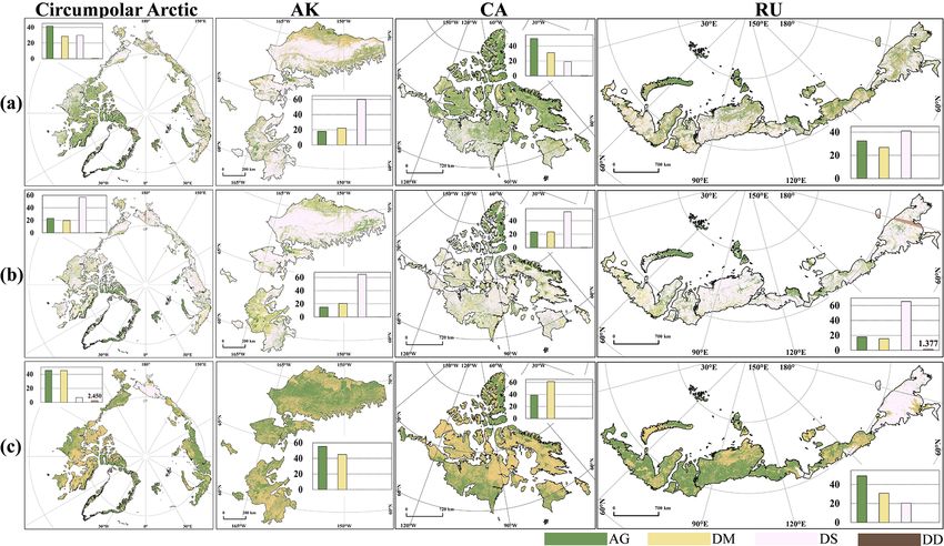
146                                                                                                               C. Liu et al.: CALC-2020

Figure 9. Circumpolar Arctic land cover estimated by the CALC-2020 map. (a) Land cover distribution at the 10 m pixel scale. Panels
(b)–(k) display the biome-specific area proportion in each 1◦ × 1◦ land tile. Panel (l) shows area statistics of all land cover types across the
terrestrial Arctic (unit of 103 km2 ). Error bars represent 95 % confidence intervals.

system over the terrestrial Arctic (Bartsch et al., 2016). For            polar Arctic Vegetation Map (CAVM) (Walker et al., 2005;
example, the widely used IGBP classification system (Friedl               Raynolds et al., 2019), thus carrying the potential for dis-
et al., 2010; Loveland and Belward, 1997) contains 17 cat-                criminating Arctic plant communities at a fine spatial resolu-
egories, but very few of them appear at the northern high                 tion. However, it is worth noting that some biomes exhibit
latitudes (Liang et al., 2019). By contrast, some well-known              very strong intra-class variability in physiognomy, which
polar biomes (e.g. graminoid tundra and lichen/moss) are ab-              makes the proposed classification scheme less desirable. For
sent in existing global land cover products (Fig. 8), mak-                example, a short shrubland tundra environment is a funda-
ing the description of complex landscape oversimplified.                  mentally different ecosystem from a tall one, and this influ-
In the present study, we designed a 10-category classifica-               ences a vast array of biotic and abiotic processes (Walker et
tion scheme that is generally consistent with the Circum-                 al., 2005). With updates of more multi-source Earth observa-

Earth Syst. Sci. Data, 15, 133–153, 2023                                                      https://doi.org/10.5194/essd-15-133-2023
C. Liu et al.: CALC-2020                                                                                                          147

Figure 10. Circumpolar Arctic land cover composition disaggregated at country (a) and bioclimate zone (b) scales using the map-based
area estimation strategy. Subzones A–E correspond to the following SWI sections: SWI < 6, 6 ≤ SWI < 9, 9 ≤ SWI < 12, 12 ≤ SWI < 20
and SWI ≥ 20 (in units of ◦ C). Country abbreviations are given in Sect. 2.1.

Figure 11. Box plots showing the contribution variation among different feature domains at the country level. The feature importance is
measured by the total decrease in the Gini impurity index over all trees in the RFC model.

tion data in the future (e.g. vegetation height), the develop-             Generating reliable training and validation data has al-
ment of a version 2 CALC product will become a possible                 ways been a critical constraint on land cover mapping ap-
topic, which is expected to have a hierarchical classification          plications. Traditionally, training samples can either be col-
scheme and improved mapping performances for some spe-                  lected from field surveys (Gong et al., 2020a) or interpreted
cific biomes (e.g. shrub tundra).                                       from remotely sensed images (Liu et al., 2019; Brown et al.,

https://doi.org/10.5194/essd-15-133-2023                                                     Earth Syst. Sci. Data, 15, 133–153, 2023
148                                                                                                         C. Liu et al.: CALC-2020

Figure 12. Satellite-observed afforestation in the Arctic. (a) Location of afforestation centred at 67.1◦ N, 160.2◦ W. (b) Annual median
Landsat NDVI time series from 1984 to 2021. (c, d) Comparison of two VHR images acquired in 2007 and 2018, respectively (© Google
Earth). (e) Forest extent derived from the CALC-2020 map. The topographic map was generated using the ESRI basemap layer product.

2020; Potapov et al., 2022). These approaches, however, are           unbiased information for land cover mapping accuracy as-
laborious or even unrealistic in remote and inaccessible ar-          sessment (Gong, 2008). Unfortunately, these networks are
eas, such as the Arctic. Alternatively, several studies demon-        currently sparse in the Arctic, and the site number of some
strated the potential of deriving training samples from pre-          land cover types is very limited (Table S2, Fig. 5), making
existing knowledge (Gray and Song, 2013; Hakkenberg et                them less representative for pan-Arctic applications. Com-
al., 2020). Building on this premise, our study developed a           paring the CALC-2020 map with existing global land cover
ready-for-use training sample by leveraging the FAST library          products is complementary to the sample/in situ evaluation
and pre-existing land cover datasets for supervised classifi-         in characterizing pixel-level agreement, and we found mul-
cation model development. This sample migration strategy              tiple factors (DM, DS and DD) that can cause the mapping
can be applied to various ecological zones and is particu-            inconsistency (Table 2, Fig. 6). Along with these factors, DM
larly useful in ecoregions where land cover reference data            represents the only common algorithm mechanism across all
are not available. In addition to the sample-based validation,        compared products. Rather than adopting a universal predic-
we also evaluated the CALC-2020 product with other two                tive framework for the entire study area, the land cover class
assessment data sources: in situ records and contemporary             prediction of the CALC-2020 map was derived from locally
land cover products. With precisely known locations and rel-          adaptive (country-specific) RFC models, so the unfavourable
atively homogeneous biome footprints, near-ground site net-           impacts incurred by geographical variability can be largely
works (e.g. FLUXNET and PhenoCam) provide the most                    reduced (X. Zhang et al., 2021; Huang et al., 2022). However,

Earth Syst. Sci. Data, 15, 133–153, 2023                                                https://doi.org/10.5194/essd-15-133-2023
C. Liu et al.: CALC-2020                                                                                                          149

the use of country-specific RFC models inevitably caused          on a ready-for-use training sample set derived from mul-
the spatial discontinuity issue in borderlands of neighbouring    tiple sources, the CALC-2020 map was generated through
countries, which requires further methodological improve-         a locally adaptive machine-learning classification proce-
ments in the future.                                              dure. Accuracy assessments reveal the reliability of CALC-
   Arctic ecosystem function is highly dependent on land          2020, as well as its representativeness for characterizing
cover composition and distribution; yet both of them remain       the Arctic ecosystem in ways that are not well represented
poorly understood (A’Campo et al., 2021; Wang and Friedl,         by pre-existing products. According to our estimation, the
2019; Beamish et al., 2020). We expect that the CALC-2020         graminoid tundra and lichen/moss occupy the largest Arc-
product will help fill the scientific gap by providing the most   tic land area, and the latitudinal shift of land cover composi-
recent circumpolar biophysical conditions in the Northern         tion is generally consistent with the SWI gradient profile. Our
Hemisphere. For example, accurate land cover data are key         mapping results also offer the evidence of woody encroach-
inputs for projecting biogeochemical cycles under current         ment, especially in Alaska and southern Nenets, Russia. We
and future scenarios, thus guiding local, national and global     concluded that the new CALC-2020 map can be used to aug-
efforts of climate change mitigation (Horvath et al., 2021;       ment the modelling of both biotic and abiotic processes, thus
Y. Zhang et al., 2021). Previous studies have found a pole-       enlightening innovative Arctic management.
ward movement of the Arctic treeline (the northernmost edge
of the habitat where trees are capable of growing). Our esti-
mation that circumpolar Arctic forest cover reaches approxi-      Supplement. The supplement related to this article is available
mately 32 000 km2 suggests woody encroachment as the cli-         online at: https://doi.org/10.5194/essd-15-133-2023-supplement.
mate warms and is thus consistent with the forest growth
trend (Harsch et al., 2009; Rees et al., 2020). However, our
results differ from previous studies by identifying the subtle    Author contributions. ChL, CaL and HH carried out the analy-
distribution pattern of trees with a much finer spatial resolu-   sis and wrote the manuscript. XX and XF helped with the data pro-
                                                                  cessing and the accuracy assessment. XC conceived the study. All
tion (Fig. 12). Finally, using the CALC-2020 product as the
                                                                  authors helped revise the manuscript.
baseline, along with decades of a wealth of satellite observa-
tion, circumpolar land cover change monitoring can possibly
be crafted, which will advance our understanding of a contin-
                                                                  Competing interests. The contact author has declared that none
uously changing Arctic and its global environmental impacts.      of the authors has any competing interests.

4   Data availability
                                                                  Disclaimer. Publisher’s note: Copernicus Publications remains
The CALC-2020 product generated in this paper is available        neutral with regard to jurisdictional claims in published maps and
                                                                  institutional affiliations.
through the Science Data Bank repository. The registered
database DOI is https://doi.org/10.57760/sciencedb.01869
(Xu et al., 2022a). Across the entire Arctic, the CALC-2020
                                                                  Special issue statement. This article is part of the special issue
product consists of six files in GeoTIFF format with a 10 m
                                                                  “Extreme environment datasets for the three poles”. It is not associ-
spatial resolution (EPSG: 6931). Each land cover map file is      ated with a conference.
named based on the following rule: “CALC-2020-X.tif”. The
“X” in the file name represents its mapping country (AK,
CA, GR, IC, NO, RU). Country abbreviations are given in           Acknowledgements. We acknowledge the Google Earth Engine
Sect. 2.1 of this paper. The valid values for circumpolar Arc-    platform, which makes circumpolar Arctic-scale geospatial map-
tic land cover types are 1–10. The CALC-2020 product was          ping and analysis possible at fine spatial resolutions. We are also
generated on the GEE platform using the JavaScript language       grateful to all data providers that have been used in this study. The
developed by the authors. All other data used in this study are   authors would like to thank the topical editor, Xiao Zhang and one
available from the corresponding authors upon reasonable re-      anonymous referee for their constructive and insightful comments
quest.                                                            on an earlier draft of this paper.

5   Conclusions                                                   Financial support. The   research was supported by the
                                                                  Open Research Program of the International Research Cen-
A thorough understanding of the Arctic terrestrial surface        ter of Big Data for Sustainable Development Goals (grant
requires information about both the composition and the           no. CBAS2022ORP04), the National Key R&D Program of
distribution of land cover. In this study, we developed a         China (grant nos. 2018YFC1407103, 2019YFC1509105 and
circumpolar Arctic land cover product for circa 2020 us-          2019YFC1509104), Guangdong Natural Science Foundation (grant
ing fine-resolution multi-source remote sensing data. Based       no. 2022A1515010924) and the Major Key Project of PCL.

https://doi.org/10.5194/essd-15-133-2023                                             Earth Syst. Sci. Data, 15, 133–153, 2023
You can also read