The fate of upwelled nitrate off Peru shaped by submesoscale filaments and fronts
←
→
Page content transcription
If your browser does not render page correctly, please read the page content below
Biogeosciences, 18, 3605–3629, 2021
https://doi.org/10.5194/bg-18-3605-2021
© Author(s) 2021. This work is distributed under
the Creative Commons Attribution 4.0 License.

The fate of upwelled nitrate off Peru shaped by submesoscale
filaments and fronts
Jaard Hauschildt1 , Soeren Thomsen1,2 , Vincent Echevin2 , Andreas Oschlies1 , Yonss Saranga José1 , Gerd Krahmann1 ,
Laura A. Bristow3,4 , and Gaute Lavik3
1 GEOMAR    Helmholtz Centre for Ocean Research Kiel, Kiel, Germany
2 Laboratoired’Océanographie et du Climat, Expérimentations et Approches Numériques (LOCEAN), Institut de Recherche
pour le Développement (IRD), Institut Pierre-Simon Laplace (IPSL), Université Pierre et Marie Curie (UPMC), Paris, France
3 Department of Biogeochemistry, Max Planck Institute for Marine Microbiology, Bremen, Germany
4 Department of Biology/Nordcee, University of Southern Denmark (SDU), Odense, Denmark

Correspondence: Jaard Hauschildt (jhauschildt@geomar.de)

Received: 27 March 2020 – Discussion started: 14 April 2020
Revised: 24 February 2021 – Accepted: 18 March 2021 – Published: 17 June 2021

Abstract. Filaments and fronts play a crucial role for a net       fying further analysis of nitrate uptake and subduction us-
offshore and downward nutrient transport in Eastern Bound-         ing the model. Virtual Lagrangian floats were released in the
ary Upwelling Systems (EBUSs) and thereby reduce regional          subsurface waters along the shelf and biogeochemical vari-
primary production. Most studies on this topic are based on        ables tracked along the trajectories of floats upwelled near
either observations or model simulations, but only seldom          the coast. In the submesoscale-permitting (1/45◦ ) simula-
are both approaches are combined quantitatively to assess          tion, 43 % of upwelled floats and 40 % of upwelled nitrate are
the importance of filaments for primary production and nu-         subducted within 20 d after upwelling, which corresponds to
trient transport. Here we combine targeted interdisciplinary       an increase in nitrate subduction compared to a mesoscale-
shipboard observations of a cold filament off Peru with            resolving (1/9◦ ) simulation by 14 %. Taking model biases
submesoscale-permitting (1/45◦ ) coupled physical (Coastal         into account, we give a best estimate for subduction of up-
and Regional Ocean Community model, CROCO) and bio-                welled nitrate off Peru between 30 %– 40 %. Our results sug-
geochemical (Pelagic Interaction Scheme for Carbon and             gest that submesoscale processes further reduce primary pro-
Ecosystem Studies, PISCES) model simulations to (i) evalu-         duction by amplifying the downward and offshore export of
ate the model simulations in detail, including the timescales      nutrients found in previous mesoscale studies, which are thus
of biogeochemical modification of the newly upwelled wa-           likely to underestimate the reduction in primary production
ter, and (ii) quantify the net effect of submesoscale fronts       due to eddy fluxes. Moreover, this downward and offshore
and filaments on primary production in the Peruvian up-            transport could also enhance the export of fresh organic mat-
welling system. The observed filament contains relatively          ter below the euphotic zone and thereby potentially stimulate
cold, fresh, and nutrient-rich waters originating in the coastal   microbial activity in regions of the upper offshore oxygen
upwelling. Enhanced nitrate concentrations and offshore ve-        minimum zone.
locities of up to 0.5 m s−1 within the filament suggest an off-
shore transport of nutrients. Surface chlorophyll in the fil-
ament is a factor of 4 lower than at the upwelling front,
while surface primary production is a factor of 2 higher. The      1   Introduction
simulation exhibits filaments that are similar in horizontal
and vertical scale compared to the observed filament. Ni-          The eastern margins of the subtropical oceans are character-
trate concentrations and primary production within filaments       ized by upwelling of cold and nutrient-rich subsurface wa-
in the model are comparable to observations as well, justi-        ters, caused by persistent along-shore winds that drive an off-
                                                                   shore Ekman transport. The nutrients supplied to the sunlit

Published by Copernicus Publications on behalf of the European Geosciences Union.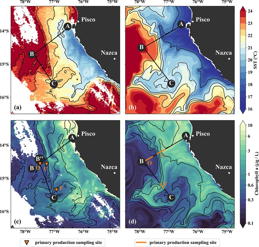
3606                              J. Hauschildt et al.: The fate of upwelled nitrate off Peru shaped by filaments and fronts

surface ocean subsequently fuel high phytoplankton growth,         to play a role in limiting primary production in the PCUS
which supports a rich ecosystem (Pennington et al., 2006).         (Hutchins et al., 2002; Bruland et al., 2005; Browning et al.,
These Eastern Boundary Upwelling Systems (EBUSs) are               2018). Furthermore, most of these studies are purely based
found in all major ocean basins and are named after the Ca-        on models, and comparison to observations has proven diffi-
nary, Benguela, California, and Peru–Chile current systems.        cult due to the difficulties of observing vertical velocities. Re-
The Peru–Chile upwelling system (PCUS) is the most pro-            gional simulations are often primarily validated using surface
ductive EBUS in the global ocean, accounting for 10 % of           chlorophyll maps derived from ocean color, which does not
the global fish catch while occupying only 0.1 % of the ocean      allow the resolution of the underlying physical (e.g., subduc-
surface (Chavez et al., 2008). The Peru upwelling ecosys-          tion) and biogeochemical processes (e.g., primary produc-
tem and the fisheries that depend on it have immense eco-          tion, hereafter PP). When attempting to quantify the effect
nomical importance for the local population. Furthermore,          of subduction on biogeochemistry using models, we need to
the high productivity and export of organic matter and its         ensure that the timescales of PP and subduction are realis-
subsequent remineralization at depth result in high rates of       tic: for instance, if the timescale of nitrate uptake by PP was
oxygen consumption (Kalvelage et al., 2015; Loginova et al.,       shorter than the subduction timescale, more organic matter
2019). In combination with poor ventilation by sluggish cur-       (produced in the surface layer) than nitrate would be sub-
rents, this leads to the presence of the shallowest and most       ducted. If it was longer, the opposite would be true. When
intense oxygen minimum zone (OMZ) in the global ocean              attempting to quantify the effect of subduction on biogeo-
(Wyrtki, 1962; Paulmier et al., 2006; Karstensen et al., 2008;     chemistry using models, we therefore need to ensure that the
Stramma et al., 2010). Besides being regions of high produc-       timescales of PP and subduction are realistic. Dedicated stud-
tivity, EBUSs are also globally relevant as natural sources of     ies combining multi-disciplinary observations with modeling
greenhouse gases to the atmosphere such as N2 O (Friederich        efforts at the meso- and submesoscale are key to advance
et al., 2008; Arévalo-Martínez et al., 2015) and CO2 (Chavez       our understanding of complex physical–biogeochemical in-
et al., 2007; Gruber, 2015; Köhn et al., 2017; Brady et al.,       teractions (Oschlies et al., 2018). Evaluating the models at
2019).                                                             these scales allows trust in the simulation of submesoscale
   Mesoscale eddies have in the past been assumed to gen-          processes to be gained to assess the associated uncertainties
erally enhance biological productivity in the open ocean by        and possible systematic biases.
either exposing nutrient-rich subsurface water to the well-lit        The degree to which dynamical processes of a certain
euphotic zone or by lateral advection of nutrients (Falkowski      scale are represented in a simulation depends on the ef-
et al., 1991; Oschlies and Garçon, 1998; Oschlies, 2002).          fective horizontal resolution of the numerical model (Capet
Conversely, in the highly productive EBUS, eddies and fil-         et al., 2008a; Soufflet et al., 2016). So far, coupled physical–
aments have been shown to decrease productivity by export-         biogeochemical model simulations focusing on eddy fluxes
ing nutrients and organic matter offshore and downward be-         of biogeochemical tracers (e.g., Nagai et al., 2015, for the
low the euphotic zone (Rossi et al., 2008, 2009; Lathuilière       California EBUS) have been limited to a horizontal resolu-
et al., 2010; Gruber et al., 2011; Nagai et al., 2015). Such       tion of ∼ 5 km in mid-latitudes, which is not sufficient to rep-
features are ubiquitous in the PCUS (Penven et al., 2005; Co-      resent submesoscale dynamics as the effective resolution of a
las et al., 2012; Thomsen et al., 2016a, b; Pietri et al., 2013;   model is much lower due to strong kinetic-energy dissipation
McWilliams et al., 2009). As the upwelling front meanders          at the smallest resolved scales (Soufflet et al., 2016). Various
and eventually becomes unstable, an ageostrophic secondary         purely physical model simulations (Capet et al., 2008b; Co-
circulation develops in order to restore geostrophic balance       las et al., 2012) and idealized biogeochemical simulations
(Thomas et al., 2008; McWilliams et al., 2009, 2015). This         (Lathuilière et al., 2010) suggest that an increase in the hor-
ageostrophic flow field can drive large vertical velocities and    izontal resolution leads to further enhancement of horizontal
thus impact the physical–biogeochemical coupling by mod-           and vertical fluxes.
ifying vertical and lateral transports of nutrients and organic       In this study, we focus on filaments and fronts which con-
matter (Lapeyre and Klein, 2006; Lévy et al., 2012; Mahade-        stitute the upper end of the submesoscale variability spec-
van, 2015). The downward fluxes can be understood as sub-          trum with length scales of O(1–10) km (McWilliams, 2016).
duction of surface water along isopycnals.                         A quantification of the net effect of filaments and subme-
   Previous studies have attempted to quantify the fluxes of       soscale frontal processes on the offshore and downward nu-
biogeochemical tracers related to eddies and filaments in          trient transport and PP off Peru is missing so far. Therefore,
EBUSs using biogeochemical models of various complex-              we address the following questions:
ity (e.g., in the California EBUS – Nagai et al., 2015; in the
                                                                     1. What is the fate of the upwelled nitrate? In particular,
PCUS – Frenger et al., 2018; Montes et al., 2014; Betten-
                                                                        what is the amount of nitrate subduction, and how does
court et al., 2015; and José et al., 2017; in the Canary EBUS –
                                                                        it impact PP?
Lovecchio et al., 2018; in the Benguela EBUS – Schmidt and
Eggert, 2016). One aspect previous model studies have not            2. What is the impact of horizontal model resolution on
addressed are the eddy fluxes of iron, a tracer which is known          subduction and PP?

Biogeosciences, 18, 3605–3629, 2021                                                   https://doi.org/10.5194/bg-18-3605-2021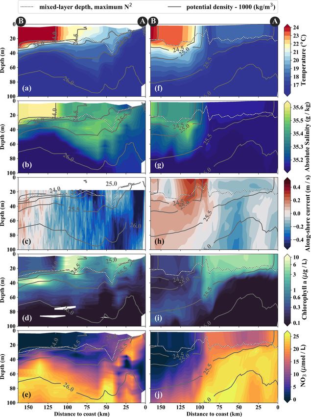
J. Hauschildt et al.: The fate of upwelled nitrate off Peru shaped by filaments and fronts                                3607

   To address these questions, we evaluate the model based        a northwest direction (BIO, BIO2). A dense sampling strat-
on physical and biogeochemical observations of a cold fil-        egy with 8–10 km horizontal spacing between stations and
ament. To assess the timescale of phytoplankton growth in         5–10 m vertical spacing between samples was applied on the
our model, we will compare PP and nutrient concentrations         biogeochemical transects. The physically underway transects
in a modeled filament with observational data. Then, we will      (PHY, PHY2) were completed overnight in under 8 h, sam-
quantify how much of the upwelled nitrate off Peru is sub-        pling with a horizontal spacing of under 1 km, similar to
ducted below the euphotic zone without being utilized by bi-      the resolution of the binned acoustic Doppler current pro-
ology.                                                            filer (ADCP) data. These physical data thus closely represent
   This paper is structured as follows: in Sect. 2 the filament   a synoptic view of the surface ocean. Sampling on the bio-
survey, the coupled physical–biogeochemical model, and all        geochemical transects (BIO, BIO2) was done during daytime
other data sources as well as analysis methods are described.     following each physical transect. Wind speed and direction
In Sect. 2.8 the model performance with respect to the rele-      on R/V Meteor were measured at 35.5 m height with a tem-
vant physical and biogeochemical quantities and their hori-       poral resolution of 1 min and corrected to 10 m height fol-
zontal variability is evaluated. In Sect. 3.1 and 3.2 the mean    lowing Smith (1988), similar to the procedure used by Köhn
horizontal variability in the upwelling structure and cold fil-   et al. (2017).
aments is characterized in detail in both observations and
model simulations. In Sect. 3.3 the simulation is used to an-     2.2   Oceanographic biophysical measurements
alyze pathways and timescales of nitrate export, subduction,
and uptake and to compare model results against estimates         Hydrographic data were obtained from lowered conductiv-
from observations. In Sect. 3.4 the effect of submesoscale-       ity, temperature, and pressure (CTD) measurements using a
permitting vs. mesoscale model resolution with respect to the     SeaBird SBE 9-plus CTD system equipped with two sets of
simulated mean biogeochemical tracer fields is analyzed. Fi-      pumped sensors. Water samples for oxygen, nutrients, and
nally, the results are discussed in the context of the existing   salinity were taken using 24 Niskin bottles (10 L) mounted
literature in Sect. 4, which also includes a detailed discus-     on a General Oceanics rosette. Salinity samples were an-
sion of the limitations of our approach. Concluding remarks       alyzed on board with a Guildline Autosal 8 model 8400B
follow in Sect. 5.                                                salinometer to calibrate conductivity measurements to prac-
                                                                  tical salinity (PSS-78) with an uncertainty of 0.003 g kg−1 .
                                                                  Practical salinity was converted to absolute salinity (TEOS-
2     Data and methods                                            10) using routines of the Gibbs Seawater toolbox (https:
                                                                  //github.com/TEOS-10/GSW-Python, last access: 7 Septem-
2.1    Filament survey                                            ber 2020). The CTD was also equipped with an oxygen sen-
                                                                  sor and a WET Labs (USA) fluorometer. The oxygen sen-
A survey designed to investigate the biophysical coupling at      sor was calibrated to an accuracy of 1.5 µmol using Winkler
a cold filament near 14◦ S off the coast of Peru was carried      titration. As Winkler titration is not reliable in the core of
out on 12–17 April 2017 using an adaptive sampling strat-         the OMZ and tends to result in too high values (Revsbech
egy guided by real-time satellite images. The fieldwork was       et al., 2009; Kalvelage et al., 2013; Thomsen et al., 2016b),
conducted during R/V Meteor cruise M136, which started            a concentration of 0 µmol L−1 was assumed in the core of
on 11 April and ended on 29 April 2017 in Callao, Peru            the OMZ and the profiles corrected accordingly following
(Dengler and Sommer, 2017; Lüdke et al., 2020). The mea-          Langdon (2010). To determine chlorophyll a concentrations
surements were carried out in the framework of the interdis-      from the measured chlorophyll fluorescence, the original fac-
ciplinary collaborative research center SFB 754 “Climate–         tory calibration provided by the sensor manufacturer WET
Biogeochemistry Interactions in the Tropical Ocean” funded        Labs (USA) was used. For more details on the calibration
by the Deutsche Forschungsgemeinschaft (DFG). The cruise          of chlorophyll fluorescence measurements, the reader is re-
track during the survey consisted of five transects (Fig. 1a).    ferred to Loginova et al. (2016). Underway subsurface tem-
The first transect (CROSS) mapped the upwelling region            perature and salinity were measured using a Teledyne Ocean-
in the cross-shore direction with conductivity, temperature,      science (Poway, USA) RapidCAST system acquiring profiles
and depth (CTD) measurements, including biogeochemical            of the upper 70 m of the water column every 2 min, resulting
parameters (O2 , NO−        −      +
                     3 , NO2 , NH4 ) determined from water        in a horizontal resolution of 790 ± 240 m depending on the
samples. On subsequent along-shore transects, a cold fila-        vessel speed. Subsurface current velocities on R/V Meteor
ment present ∼ 100 km southeast of transect CROSS was             were recorded by a vessel-mounted acoustic Doppler current
crossed by R/V Meteor four times in a zigzag pattern: twice       profiler (vmADCP). The system used was a Teledyne RD In-
with high-resolution underway CTD measurements of physi-          struments OceanSurveyor 75 kHz ADCP capable of reaching
cal parameters heading in a southeast direction (PHY, PHY2)       a maximum depth of ∼ 700 m. The shallowest velocity mea-
and two more times with station-based lowered CTD mea-            surements were acquired in a bin centered 18 m below the
surements including biogeochemical parameters heading in          sea surface. During the filament crossing, the vessel speed

https://doi.org/10.5194/bg-18-3605-2021                                                 Biogeosciences, 18, 3605–3629, 2021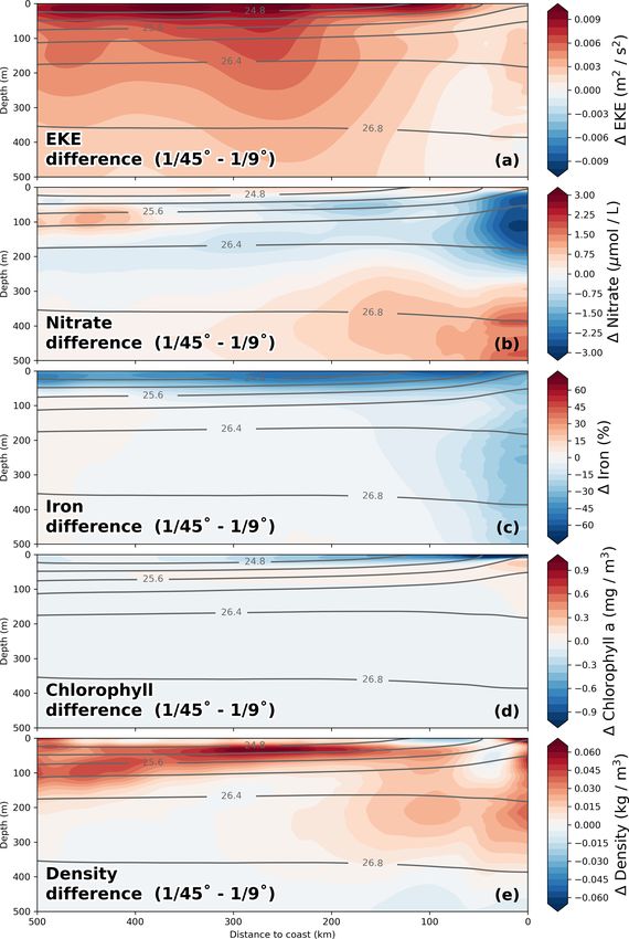
3608                             J. Hauschildt et al.: The fate of upwelled nitrate off Peru shaped by filaments and fronts

was kept nearly constant at ∼ 5 m s−1 to obtain high-quality     sampling depth. Incubations were terminated after 24 h by
velocity measurements with a vertical resolution of 8 m and a    filtration onto 25 mm pre-combusted (450 ◦ C, 4 h) GF/F fil-
horizontal resolution of 290 ± 26 m, which was subsequently      ters (Whatman), which were dried onboard (50 ◦ C, 12 h) and
averaged in 1 km bins. Nutrient concentrations were deter-       stored at room temperature until analysis. Prior to analysis,
mined onboard by a QuAAtro autoanalyzer (SEAL Analyti-           GF/F filters were acidified over fuming HCl overnight in a
cal, Southampton, UK) using standard photometric methods         dessicator, dried, and pelletized in tin cups. Samples were
(Grasshoff et al., 1983).                                        analyzed for particulate organic carbon and isotopic compo-
   During M136 a self-contained ultraviolet SUNA (sub-           sition using continuous-flow isotope ratio mass spectrometry
mersible ultraviolet nitrate analyzer) nitrate sensor manufac-   coupled to an elemental analyzer. PP rates were calculated
tured by Sea-Bird Scientific was attached to the CTD–rosette     from the incorporation of 13 C into biomass as described in
system similar to Alkire et al. (2010). SUNA sensors de-         Großkopf et al. (2012).
termine the concentration of nitrate by measuring the ab-
sorption of UV light over a fixed path length. The SUNA
                                                                 2.4   Data products
data have been reprocessed with the concurrent CTD pres-
sure, temperature, and salinity (for bromide absorption) data
to eliminate their effects on the absorption and the result-     To guide the shipboard measurements and put them into
ing nitrate concentrations (Sakamoto et al., 2009, 2017). The    a regional context, MODIS (Moderate Resolution Imaging
resulting SUNA nitrate concentrations have been extracted        Spectroradiometer) Level 2 along-track sea-surface temper-
for the times at which bottles were closed on the water sam-     ature (SST) and chlorophyll a products with an approximate
pler. These concentrations have then been compared to the        resolution of 1 km from the TERRA and AQUA satellites
nitrate and nitrite concentrations measured with the autoan-     were used (https://oceandata.sci.gsfc.nasa.gov/, last access:
alyzer. SUNA nitrate values correlated highly with the au-       23 May 2017). We restricted our analysis to daylight im-
toanalyzer values (r squared: 0.9972, with the 10 % most         ages of SST and used the cloud mask based on ocean color
deviating samples removed). SUNA values were also com-           because of obvious deficiencies of the cloud mask based
pared to the combined autoanalyzer concentrations of ni-         on infrared SST data alone. SST data from AVHRR (Ad-
trate and nitrite, but the resulting correlation was somewhat    vanced Very High Resolution Radiometer; Saha et al., 2018)
weaker (r squared: 0.9964, with the 10 % most deviating          at 25 km resolution were provided by the NOAA (National
samples removed). The SUNA measurements were thus cor-           Oceanic and Atmospheric Administration; ftp://eclipse.ncdc.
rected to match the nitrate (NO3 ) concentration by applying     noaa.gov/pub/OI-daily-v2/NetCDF/, last access: 1 Decem-
the following correction term, where NO3, old is the origi-      ber 2020). For evaluating the model performance with re-
nal measurement, and NO3, new is the final corrected value:      spect to PP, we used estimates of ocean net primary produc-
NO3, new = 1.2813 + 1.0576 × NO3, old . We applied this cal-     tion (NPP) which were derived from both MODIS and Sea-
ibration to all SUNA nitrate concentrations.                     WIFS chlorophyll a using the Vertically Generalized Produc-
   All observational datasets mentioned above (Krahmann,         tion Model (VGPM; Behrenfeld and Falkowski, 1997; http:
2018; Dengler et al., 2019a, b; Tanhua and Visbeck, 2018)        //sites.science.oregonstate.edu/ocean.productivity/, last ac-
are published at the world data center PANGAEA follow-           cess: 1 December 2020). Sea-surface height (SSH) data
ing the SFB 754 data policy (https://www.pangaea.de, last        from DUACS/AVISO (Data Unification and Altimeter Com-
access: 1 December 2020; see “Code and data availability”        bination System; Archiving, Validation and Interpretation
section).                                                        of Satellite Oceanographic data) satellite altimeter product
                                                                 (SEALEVEL_GLO_PHY_L4_REP_OBSERVATIONS_008
2.3    Incubations                                               _047) used for model evaluation were produced and dis-
                                                                 tributed at 0.25◦ resolution by the Copernicus Marine
Seawater samples were filled into 2 L polycarbonate bottles      and Environment Monitoring Service (CMEMS; https:
and were stored in the dark until tracer additions were made,    //marine.copernicus.eu, last access: 1 December 2020).
which was always within 2 h of collection. Following the         A global mixed-layer depth (MLD) climatology with
method outlined in Großkopf et al. (2012), incubations were      2◦ × 2◦ resolution based on a 0.2 ◦ C temperature cri-
started with the addition of sodium bicarbonate (NaH13 CO3 ;     terion was provided by IFREMER (de Boyer Mon-
> 98 atom %, Sigma Aldrich) to yield a final enrichment of       tégut et al., 2004; http://www.ifremer.fr/cerweb/deboyer/
approximately 3.2 at. %. At each depth sampled, three bot-       mld/Surface_Mixed_Layer_Depth.php, last access: 1 De-
tles received a 13 C addition, and a fourth bottle received no   cember 2020). Annual mean temperature and nitrate fields
13 C and acted as an untreated control, allowing the natural     for model evaluation were provided at 1/2◦ resolution by the
abundance 13 C to be determined at each depth. All bottles       CARS climatology (CSIRO Atlas of Regional Seas, Ridg-
were placed into on-deck incubators with surface seawater        way et al., 2002; http://www.marine.csiro.au/atlas/, last ac-
flow-through and shaded with 20 %, 10 %, or 1 % surface ir-      cess: 1 December 2020). Annual mean gridded chlorophyll a
radiance (Lee Filters, Seattle, WA, USA), depending on the       products from the MODIS and SeaWIFS satellite-based in-

Biogeosciences, 18, 3605–3629, 2021                                                https://doi.org/10.5194/bg-18-3605-2021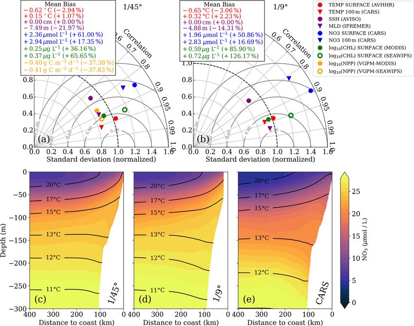
J. Hauschildt et al.: The fate of upwelled nitrate off Peru shaped by filaments and fronts                                  3609

struments were downloaded from NOAA (https://oceandata.           Data Set) (Worley et al., 2005) climatology relaxed to
sci.gsfc.nasa.gov/, last access: 1 December 2020).                AVHRR (Advanced Very High Resolution Radiometer; ftp://
                                                                  eclipse.ncdc.noaa.gov/pub/OI-daily-v2/NetCDF/) daily SST
2.5   Physical model (CROCO)                                      according to

We employed CROCO (Coastal and Regional Ocean Com-                                 dQ
munity model) to study the circulation in the PCUS                Q = QCOADS +        · (SSTCROCO − SSTAVHRR ),               (1)
                                                                                   dT
at submesoscale-permitting resolution. CROCO is a free-
surface, terrain-following coordinate ocean modeling system          where dQdT represents the additional heat flux that is im-
built upon ROMS_AGRIF (Penven et al., 2006; Shchepetkin           posed per degree of temperature difference between model
and McWilliams, 2009) and a non-hydrostatic kernel (not           SST and observed SST. This heat flux correction is a func-
used in this study). CROCO solves the primitive equations         tion of atmospheric parameters and assumes values of −30–
using the Boussinesq approximation and a hydrostatic verti-       35 W/m2 /◦ C (Barnier et al., 1995). The model was forced
cal momentum balance. The nonlocal K-profile parameteri-          with surface wind stress derived from the daily level 2 wind
zation (KPP) scheme is used to handle unresolved processes        product provided by the advanced scatterometer (ASCAT)
related to vertical mixing. For a complete description of the     (https://podaac.jpl.nasa.gov/dataset/ASCATB-L2-25km).
model numerical schemes the reader can refer to Shchep-
etkin and Mcwilliams (2005). The code used in the present         2.6   Biogeochemical model (PISCES)
study is the CROCO v1.0 version, which is very similar to
ROMS_AGRIF version v3.1.                                          The CROCO model was coupled to the PISCES (Pelagic In-
   The model was configured as a nested set of two spatial        teraction Scheme for Carbon and Ecosystem Studies) bio-
domains (Fig. 1b) using an offline one-way embedding pro-         geochemical model, which simulates the biogeochemical cy-
cedure (Mason et al., 2010). The outer domain has a reso-         cles of carbon and the main nutrients (P, N, Si, Fe). It in-
lution 1/9◦ over a region of 2207 km in the zonal direction       cludes two phytoplankton compartments (nanophytoplank-
by 2911 km in the meridional direction (24.4 ◦ × 26.2 ◦ ), and    ton and diatoms), two zooplankton size classes (microzoo-
the inner domain has a resolution of 1/45◦ over a region of       plankton and mesozooplankton), two detritus classes, and a
918 km in the zonal direction by 973 km in the meridional         description of the carbonate chemistry. A detailed model de-
direction (8.69 ◦ × 8.76 ◦ ). Since the Peruvian upwelling sys-   scription is given in Aumont et al. (2015). In the following
tem is located relatively close to the Equator, the Rossby ra-    we outline only the equations that are relevant for our analy-
dius is about 70 km in our study area (Chelton et al., 1998),     sis of the local temporal nitrate changes.
more than an order of magnitude larger than our model res-           The evolution of nitrate in PISCES is determined by
olution (∼ 2.5 km). The Rossby radius effectively represents      Eq. (2), with the right-hand side terms representing nitrate in-
the limit of mesoscale dynamics, and we can thus consider         crease due to nitrification and nitrate loss due to small phyto-
our model submesoscale-permitting as it resolves the up-          plankton growth, large phytoplankton growth, and denitrifi-
per range of the submesoscale variability spectrum. There         cation (we omitted the physical transport and mixing terms):
are 32 sigma levels, and the vertical resolution varies with
water depth. Here we focus on the upper 200 m of the wa-          ∂NO3
                                                                       = nitrification − µPNO3 P − µD
                                                                                                    NO3 D − denitrification.
ter column, where the vertical resolution near the surface is      ∂t
1–2 m (5 m) on the shelf (offshore). The model topography                                                                 (2)
was derived from the GEBCO (General Bathymetric Chart
                                                                    The nitrate uptake rate of small phytoplankton P , µPNO3 is
of the Oceans; http://www.gebco.net) product, interpolated
                                                                  defined by Eq. (3) as follows:
onto the model grid and smoothed to reduce pressure gradi-
ent errors.                                                                        LPNO3
   The lateral open-boundary conditions of the outer do-          µPNO3 = µP                   .                              (3)
main for temperature, salinity, velocities, and sea level were                 LPNO3 + LPNH4
provided at 1/12 ◦ resolution by the MERCATOR PSY4V2
                                                                  The limitation term for nitrate LPNO3 is described by Eq. (4):
model (Lellouche et al., 2018), which assimilated in situ data
transmitted from R/V Meteor during the research cruises                                     P NO
                                                                                           KNH   3
M135 (large-scale mapping off the OMZ; Tanhua and Vis-            LPNO3 =                     4
                                                                             P K P + K P NO + K P NH
                                                                                                                   .          (4)
beck, 2018) and M136 (Krahmann, 2018) and from ARGO                         KNO3 NH4  NH4  3   NO3   4
floats (http://www.argo.ucsd.edu/) as well as satellite SST
and sea-level measurements. No assimilation or “nudging”          The limitation term for ammonium LPNH4 is similar to Eq. (4)
was done inside the model domain except for a restoring           but with the product of ammonium concentration NH4 and
                                                                                            P
                                                                  half-saturation constant KNO    in the numerator. The half-
term on the surface heat flux. The net surface heat flux Q is                                   3
given by the COADS (Comprehensive Ocean–Atmosphere                saturation constants for nitrate KNOP   and for ammonium
                                                                                                        3

https://doi.org/10.5194/bg-18-3605-2021                                                    Biogeosciences, 18, 3605–3629, 2021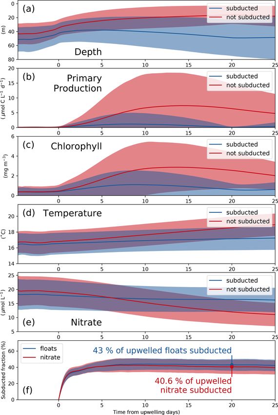
3610                                  J. Hauschildt et al.: The fate of upwelled nitrate off Peru shaped by filaments and fronts

Figure 1. (a) Observed SST (MODIS) on 14 April 2017 with cruise track and section names superimposed. (b) Model SST on 14 April 2017
in the coarse- (1/9 ◦ ) and high-resolution (1/45 ◦ ) CROCO simulations superimposed on AVHRR satellite SST. Black rectangles indicate
the respective model domains.

  P
KNH   set the concentrations at which the limiting effect of         these nutrients are added before calculating the total nutri-
    4
each nutrient would result in half the maximum uptake rate.          ent limitation term. The equations for the nitrate uptake rate
The growth rate for small phytoplankton P , µP is described          of large phytoplankton D, µD   NO3 (see Eq. 2) have an identi-
by Eq. (5):                                                          cal structure to Eqs. (3)–(6) and are therefore omitted here.
                                                                     Primary production is proportional to the sum of the small
µP = µ0max f1 (T )f2 (Lday , zmxl )                                  phytoplankton biomass P and large phytoplankton biomass
                                                                     D, multiplied by their respective growth rates µP and µD .
                                         !!
                −α P θ chl,P PARP
       1 − exp                                LPlim ,         (5)       The open-boundary conditions for oxygen, nitrate, phos-
               Lday µ0max f1 (T )LPlim
                                                                     phate, and silicate were provided at 1/2◦ resolution by the
where µ0max is the maximum growth rate at 0 ◦ C, f1 is a func-       CARS climatology (CSIRO Atlas of Regional Seas; Ridg-
tion describing the dependence on the temperature T of the           way et al., 2002) as the sum of an annual mean and both
growth rate, and PAR is photosynthetically available radia-          annual and semi-annual cycles. For the variables not avail-
tion. The function f2 introduces additional dependencies of          able from data climatologies (iron, dissolved organic and in-
the growth rate on the length of day Lday and the mixed-layer        organic carbon, total alkalinity), a climatology derived from
depth zmxl in case it exceeds the euphotic zone. The term in-        model output of a global NEMO-PISCES (Nucleus for Eu-
side the parentheses is defined so that it increases exponen-        ropean Modelling of the Ocean, Pelagic Interaction Scheme
tially with the amount of absorbed light given by the prod-          for Carbon and Ecosystem Studies) simulation at 2◦ resolu-
uct of a constant parameter α P , the variable chlorophyll-to-       tion was used (Aumont et al., 2015).
carbon ratio θ chl,P , and the photosynthetically available radi-       After a spinup of 14 years for the 1/9◦ simulation, the 1/9◦
ation PARP . The total nutrient limitation term LPlim is defined     and 1/45◦ simulations were started from this model state and
by Eq. (6):                                                          run from January 2013 until April 2017. Only model data
                                                                     from March 2014 onwards have been used in the analysis to
                                                                   allow for an additional spinup of the submesoscale dynamics
LPlim = min LPPO4 , LPNO3 + LPNH4 , LPFe ,                    (6)    in the 1/45◦ nest. The model output frequency was set to 1 d
                                                                     for the 1/45◦ simulation and to 3 d for the 1/9◦ simulation.
where LPPO4 , LPNO3 , LPNH4 , and LPFe are the respective indi-      For the Lagrangian analysis we generated additional output
vidual limitation terms for phosphate, nitrate, ammonium,            at a 4-hourly frequency from both simulations. The higher
and iron (see Aumont et al., 2015, for details). The nutrient        frequency allows for a more precise offline calculation of the
with the smallest individual limitation term (i.e., the small-       float trajectories.
est concentration relative to its half-saturation constant) is
taken to be the limiting nutrient and controls phytoplankton
growth. Since phytoplankton can use both nitrate and ammo-
nium as a nitrogen source, the individual limitation terms for

Biogeosciences, 18, 3605–3629, 2021                                                     https://doi.org/10.5194/bg-18-3605-2021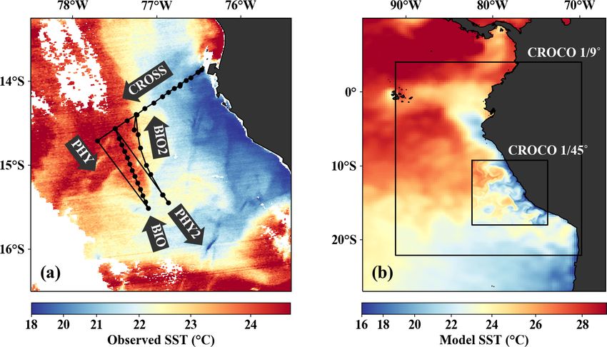
J. Hauschildt et al.: The fate of upwelled nitrate off Peru shaped by filaments and fronts                                  3611

2.7   Virtual Lagrangian float experiments                          welled floats yields the nitrate subduction ratio. Using this
                                                                    ratio we can account for the reduction in nitrate during the
To study the temporal evolution of biogeochemical proper-           time period that the subducted floats stay in the euphotic
ties in the upwelled water, an ensemble of 20 float experi-         zone. A timescale of 20 d was chosen because the number
ments was conducted. The ensemble consists of five experi-          of upwelled floats below the euphotic zone appears to have
ments, each performed in April of the years 2014–2017 and           stabilized after this time (Fig. 6f below).
initialized on day 1, 6, 11, 16, and 21. For each of these ex-
periments, 250 000 virtual Lagrangian floats were advected          2.8   Model evaluation of the annual mean fields
by the 4 h average model flow field for 35 d using the ROMS
offline tool (Capet et al., 2004; Carr et al., 2008). Virtual       In this section, we verify that the two simulations realisti-
floats were released between the coast and ∼ 250 km offshore        cally reproduce the annual mean physical and biogeochem-
over the upper 150 m, and biogeochemical variables were             ical structures. The model evaluation focuses here on the
tracked along float trajectories. Following Thomsen et al.          horizontal variability over a 2-year averaging period (2015–
(2016a) we subsampled the trajectories of all floats that were      2016). The comparison of the most relevant physical and
upwelled near the coast. We consider floats to be upwelled          biogeochemical variables with observations is summarized
when they (1) are in the euphotic zone at any given time,           in Taylor diagrams for both the 1/45◦ and 1/9◦ simulations
(2) were below the euphotic zone for at least 1 d before that       (Fig. 2a, b). The corresponding mean horizontal fields are
and at the time of release, (3) have a density higher than          shown in Figs. S1–S6.
25 kg m−3 , and (4) are located between 13 and 16◦ S. The eu-          The simulated SST shows a negative bias (∼ −0.6 ◦ C)
photic zone is defined as the upper layer of the ocean, where       relative to satellite observations for both simulations. This
photosynthetically available radiation is larger than 1 % of        negative bias is a ubiquitous feature of EBUS simulations
its surface value. The duration of 1 d was chosen somewhat          (e.g., Dufois et al., 2012) attributed partly to overly strong
arbitrarily to exclude floats that have their source at the sur-    wind-driven upwelling near the coast (Fig. S1). The spatial
face and are simply subject to relatively short, alternating        patterns of simulated and observed mean SST are highly cor-
vertical motions while they enter the upwelling patch. This         related (r = 0.95). This is expected since SST observations
is justified as the upwelling implies a source at the subsur-       are used to calculate the restoring term on the model surface
face, and the results are not sensitive to this parameter choice.   heat flux, thus partly constraining the model SST. At 100 m
The density criterion (3) is imposed to restrict our analysis to    depth, a weak positive temperature bias is found in both the
the trajectories that surface inshore of the upwelling front,       1/9◦ simulation (0.32 ◦ C) and the 1/45◦ simulation (0.15 ◦ C)
where the densest isopycnals outcrop. The regional criterion        with respect to CARS. The correlation between the model
(4) ensures that the upwelled floats originate close to the cen-    and observations at this depth is high (r > 0.9).
ter of the model domain and will only rarely reach the open            The model mixed layer is slightly shallower (−4.88 m)
boundaries during the experiment. It also serves the purpose        than the observed IFREMER climatology mixed-layer depth
of maintaining comparability with the observational data that       (de Boyer Montégut et al., 2004) in the 1/9◦ simulation,
were collected in this region.                                      while the MLD bias is slightly larger (−7.49 m) in the 1/45◦
   To analyze the fate of upwelled nitrate in more detail, we       simulation (Fig. 2a, b). The spatial variability in the mean
used the subsampled float trajectories to compute the frac-         for both simulations is well reproduced (r > 0.95), display-
tion of upwelled nitrate that is subducted. We computed a           ing a shallower mixed layer near the coast due to the shoal-
“subduction ratio” as follows:                                      ing of isotherms (Fig. S4). Note that the coarse resolution of
                                                                    the gridded MLD climatology (2◦ × 2◦ ) is a limitation for
        PNsubducted                                                 the MLD evaluation. The SSH bias for both simulations is
           i=1        NO3 i,t20
ratio = PN                        ,                          (7)    equal to zero by construction as the time-averaged and spa-
           upwelled
                      NO3 i,t0                                      tially averaged sea level has been subtracted from each time
            i=1
                                                                    series (Fig. 2a, b). Subtracting a reference value has no ef-
   where Nupwelled is the total number of upwelled floats,          fect on the pressure gradients which drive the dynamics. The
Nsubducted is the total number of subducted floats, NO3 t0 is       spatial SSH variations are only slightly underestimated in the
the nitrate concentration of each float at the time of up-          simulations (∼ −10 %), and the spatial correlation between
welling, and NO3 t20 is nitrate concentration of each float 20 d    simulated and observed SSH fields is high (r ≈ 0.8; Fig. 2a,
after upwelling. We first save the nitrate concentration for        b).
each individual float at the time of upwelling. If a float is          The simulated eddy kinetic energy (EKE) calculated from
below the euphotic zone – defined as 0.1 % surface inten-           SSH and surface geostrophy is overestimated relative to
sity PAR – 20 d after upwelling, we consider this float sub-        AVISO satellite observations for both simulations (Fig. S6).
ducted and also save the nitrate concentration at this time.        The overestimation of EKE amounts to ∼ 37 % for the 1/9◦
The sum of the nitrate concentration over the subducted floats      simulation and 100 % for the 1/45◦ simulation. There are
divided by the sum of the nitrate concentration over all up-        several possible reasons for this mismatch: firstly, the open

https://doi.org/10.5194/bg-18-3605-2021                                                   Biogeosciences, 18, 3605–3629, 2021
3612 J. Hauschildt et al.: The fate of upwelled nitrate off Peru shaped by filaments and fronts Figure 2. Taylor diagrams for (a) 1/45◦ and (b) 1/9◦ simulations, respectively. The statistics were computed from temporally averaged 2-year-mean fields (see Fig. S1) and therefore represent their spatial variability. Due to the strongly skewed distributions of chlorophyll a and PP, these variables were logarithmized prior to computing correlation and standard deviation to approximate normally distributed variables, while the mean bias was calculated using the original values. Gray concentric circles centered around unity-normalized standard deviation and correlation indicate the normalized root mean square error (NRMSE). The analysis for the 1/9◦ simulation was restricted to the extent of the 1/45◦ domain to facilitate direct comparison. Primary-production rates were not saved for the 1/9◦ simulation and could therefore not be evaluated. (c–e) Along-shore-averaged sections of mean nitrate concentrations with temperature contours superimposed for the (c) 1/45◦ simulation, (d) 1/9◦ simulation, and (e) CARS climatology. The CARS climatology was interpolated onto the 1/45◦ model grid before computing the along-shore average. boundaries of the relatively small 1/45◦ domain likely do We now evaluate the model biogeochemical fields. The not allow sufficient removal of EKE by westward propaga- model surface chlorophyll is too high in both simulations tion of eddies. Furthermore, the 2-year averaging period used relative to satellite observations, while the spatial variabil- for this model evaluation is short, and the comparison to ob- ity in chlorophyll is well reproduced (Fig. 2a,b). The positive servations is difficult due to freely evolving turbulence in the bias is reduced in the 1/45◦ simulation by a factor of 2 com- simulations. Lastly, the SSH observations are acquired along pared to the 1/9◦ simulation. Despite the positive chl bias, satellite tracks, and the mapping of this spatially and tem- the modeled PP in the 1/45◦ simulation is underestimated porally uneven data on a uniform grid can introduce biases. with respect to PP estimates derived from ocean color (bias For a fair comparison of simulated and observed EKE, the ∼ −37 %). Our in situ measurements generally suggest an sampling and processing of the satellite data would need to underestimation of PP in the simulations as well, with the be reproduced with model data. This analysis is beyond the exception of the surface values at the upwelling front (Ta- scope of this study, and we can therefore not be certain of the ble 1). extent to which the EKE in our simulations is overestimated. Biogeosciences, 18, 3605–3629, 2021 https://doi.org/10.5194/bg-18-3605-2021
J. Hauschildt et al.: The fate of upwelled nitrate off Peru shaped by filaments and fronts 3613
The model tends to overestimate nitrate at surface at the coast (σθ = 25.5 kg m−3 ) descends to 50 m depth 75–
(bias ∼ +2 µmol L−1 ) and subsurface (bias ∼ +3 µmol L−1 ) 100 km offshore. The predominant water mass along the den-
levels in both simulations (Fig. 2a, b), while the spatial pat- sity surfaces that supply the coastal upwelling is the Equa-
terns are well reproduced (Fig. S1). In general, nitrate is torial Subsurface Water (ESSW; e.g., Silva et al., 2009)
slightly improved in the 1/45◦ simulation compared to the at a density of about σθ = 26.0 kg m−3 and a salinity of
1/9◦ simulation. The modeled cross-shore vertical structure 35.2 g kg−1 (Fig. 4b), which is transported poleward along
of temperature and nitrate is also evaluated using along- the shelf by the Peru–Chile Undercurrent (PCUC; Gun-
shore-averaged mean sections from the two simulations and ther, 1936; Fonseca, 1989; Montes et al., 2010). The maxi-
from the CARS climatology (Figs. 2c–e). Above 100 m mum poleward velocities of ∼ 0.5 m s−1 are observed within
depth, the simulated isotherms compare well with the cli- 50 km from the coast at 20–100 m depth (Fig. 4c).
matology but are slightly steeper within 200 km from the The observed physical variability in the upwelling re-
coast and less steep farther offshore, suggesting a slightly too gion gives rise to biogeochemical variability on similar
strong coastal upwelling and too weak offshore upwelling scales (Figs. 3c, 4d, e). Surface chlorophyll concentrations
by Ekman suction in the simulations. Below 100 m depth, are enhanced inshore of the upwelling front (∼ 5 mg m−3 )
the isotherms slope downward towards the coast, indicative compared to offshore (∼ 0.3 mg m−3 ) due to nutrient-rich
of the Peru–Chile Undercurrent. Nitrate isolines roughly fol- subsurface waters (15–20 µmol L−1 NO3 ) that are brought
low isotherms. Modeled nitrate values are too high along the to the surface in the coastal upwelling (Figs. 3c, 4d,
continental slope above 250 m depth. Despite this bias, the e). Surface NO3 concentrations decrease continuously by
horizontal and vertical nitrate gradients above 100 m depth about 0.1 µmol L−1 per kilometer cross-shore distance to
compare well with the CARS climatology (Fig. 2c–e). We 5 µmol L−1 inshore of the upwelling front (Fig. 4e). Note
can therefore assume that the model realistically represents that a local chlorophyll maximum occurs on the cold side
the nitrate fluxes associated with upwelling and subduction, of the upwelling front (∼ 10 mg m−3 ; Figs. 3c, 4d). Off-
which occur predominantly in this depth range. Further de- shore of the upwelling front surface nutrients are depleted
tails on the model evaluation can be found in Hauschildt (< 1 µmol L−1 NO3 ), and a strong vertical gradient of up to
(2017). 2 µmol L−1 NO3 m−1 is present across the base of the mixed
layer (Fig. 4e). As a result, the maxima in chlorophyll (7–
10 mg m−3 ; Fig. 4d, Table 1) and PP (∼ 9 µmol C L−1 d−1 ,
3 Results Table 1) occur below the mixed layer, where nutrients are
abundant (20 µmol L−1 NO3 ; Fig. 4e). Below 80 m depth
3.1 Physical and biogeochemical upwelling structure in chlorophyll concentrations are low (< 0.2 mg m−3 ) every-
observations and simulations where in the study area (Fig. 4d). Due to low subsur-
face chlorophyll concentrations in the source waters on the
The filament survey (Sec. 2.1) was carried out during shelf, surface chlorophyll concentrations remain relatively
the transition from austral summer to fall during 12– low (∼ 1 mg m−3 ) within 20–30 km from the upwelling cen-
17 April 2017. Being typical for the season, moderate south- ter and only peak (4–6 mg m−3 ) farther offshore (Figs. 3c,
easterly along-shore winds between 5–6 m s−1 near the coast 4d). This illustrates that despite the clear inverse relationship
and 11–14 m s−1 offshore were observed throughout the sur- of chlorophyll and SST on larger scales, small-scale chloro-
vey, which represents upwelling-favorable conditions (not phyll variability is more complex and not consistently related
shown). The most intense upwelling is often found in dis- to SST.
tinct cells near headlands and capes, indicated by along- From the model simulation, we chose one particular event
shore minima of sea-surface temperature (SST). A well- that reproduces physical conditions similar to those of the
known upwelling cell off Peru can be identified near 15 ◦ S survey and assessed the ability of the model to capture the
by its relatively low SST (18 ◦ C) in a satellite image taken dynamics observed in situ. The characteristic structure of
on 14 April 2017, 18:25 UTC (Fig. 3a). A strong cross-shore coastal upwelling in the physical fields for this particular
SST gradient exists between this coastal minimum and the event is well reproduced in our simulations, but some differ-
warm offshore waters (24.5 ◦ C). The maximum SST gradi- ences exist (Figs. 4a–c, f–h). The location of the upwelling
ent (0.15 ◦ C/km) is found 110–130 km offshore along the front 100 km offshore and the corresponding 1 SST maxi-
23 ◦ C isotherm and marks the location of the upwelling mum of 0.2 ◦ C km−1 agrees well with both satellite images
front. The offshore increase in SST is accompanied by an in- and in situ measurements (Figs. 3a, b, 4a, f). The temper-
crease in salinity from 35.3 to 36.25 g kg−1 and an increase in ature and salinity distributions are, overall, similar to ob-
mixed-layer depth from 5 to 30 m, approximately following servations in the simulation, apart from a cold and fresh
the σθ = 25 kg m−3 isopycnal (Fig. 4a). Offshore of the up- bias of the surface waters inshore of the upwelling front
welling front, a sharp thermocline with vertical temperature (Figs. 4a, b, f, g). Due to this bias the σθ = 25 kg m−3 isopy-
gradients of up to 0.4 ◦ C m−1 across the base of the mixed cnal outcrops 100 km offshore in the simulation and near
layer is found (Fig. 4a). The deepest isopycnal that outcrops the coast in the observations. The average mixed-layer depth
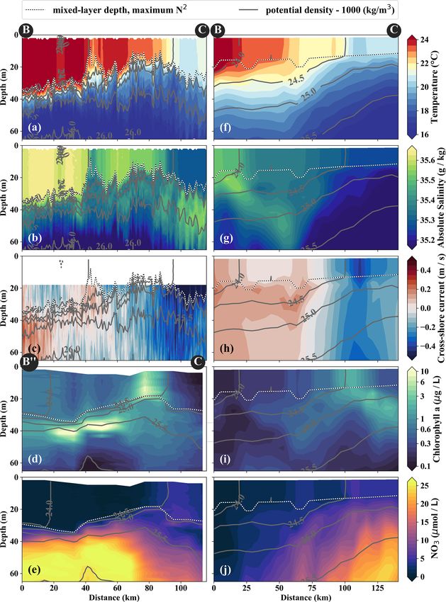
https://doi.org/10.5194/bg-18-3605-2021 Biogeosciences, 18, 3605–3629, 20213614 J. Hauschildt et al.: The fate of upwelled nitrate off Peru shaped by filaments and fronts Figure 3. (a, b) Sea-surface temperature and (c, d) surface chlorophyll in (a, c) observations on 14 April 2017 and in (b, d) the model simulation on 5 April 2017. Locations of vertical sections are superimposed (see Figs. 4, 5). Orange triangles in (c) indicate three sampling locations – offshore (O), at the upwelling front (U), and in the filament (F) – where primary production was measured. Orange lines in (d) indicate the corresponding locations used for comparison in the simulation. The simulated fields represent 1 d averaged model output. in the simulation is ∼ 20 m, very close to observed values PCUC, which is close to the observed velocity (∼ 14 cm s−1 ; offshore of ∼ 100 km. However, the observed mixed-layer Chaigneau et al., 2013). depth decreases to only ∼ 5 m in the coastal upwelling patch, In the simulation, the upwelling structure also dominates whereas such a shallow mixed layer is not seen in the sim- the variability in the biogeochemical fields (Figs. 3d, 4i, ulation (Fig. 4a, f). The southward velocities of ∼ 0.3 m s−1 j). Chlorophyll concentrations above 0.2 mg m−3 are found inshore of the upwelling front in the simulation that are as- down to 80 m (100 m) in the observations (simulation), show- sociated with the surfacing undercurrent are similar to ob- ing overall good agreement (Fig. 4d, i). Maximum surface servations (Fig. 4c, h). However, the strongest southward chlorophyll values in the observations (> 10 mg m−3 ) and flow (∼ 0.3 m s−1 ) in the simulation is weaker than observed in the simulation (∼ 8 mg m−3 ) are also reasonably similar. (∼ 0.5 m s−1 ) and not located at the shelf but 55 km off- However, the cross-shore and vertical gradients of surface shore. This is likely related to differences in mesoscale vari- chlorophyll reveal notable differences between the observa- ability since an anticyclone is present immediately offshore tions and the simulation: local maxima of up to 10 mg m−3 of the upwelling patch in the simulation compared to a cy- are present along the nutricline and at the upwelling front lo- clonic eddy at approximately the same position in the obser- cated more than 100 km offshore in the observations, while vations (not shown). Averaging over the period 2015–2016 chlorophyll concentrations in the simulation show no such yields an alongshore velocity of 13 cm s−1 in the core of the maxima, are inversely related to SST, and decrease almost Biogeosciences, 18, 3605–3629, 2021 https://doi.org/10.5194/bg-18-3605-2021
J. Hauschildt et al.: The fate of upwelled nitrate off Peru shaped by filaments and fronts                                                   3615

Figure 4. Cross-shore sections of (a, f) temperature, (b, g) salinity, (c, h) along-shore current, (d, i) chlorophyll, and (e, j) nitrate in obser-
vations (a–e) and model simulations (f–j). Potential-density contours are shown in gray, and mixed-layer depth is represented by the broken
white–black line. Letters A and B indicate the section endpoints marked in Fig. 3. The model sections represent 1 d averaged output on
14 April 2017.

https://doi.org/10.5194/bg-18-3605-2021                                                               Biogeosciences, 18, 3605–3629, 2021
3616                             J. Hauschildt et al.: The fate of upwelled nitrate off Peru shaped by filaments and fronts

continuously offshore and with depth (Fig. 3, 4d, i). Lastly,     contains recently upwelled water, which is transported to the
it is a common feature in satellite images of chlorophyll         open ocean by an offshore flow of up to 0.5 m s−1 within the
that concentrations remain relatively low (< 1 mg m−3 ) in        mixed layer (Figs. 5c). The subsurface flow is mainly off-
recently upwelled waters near the coast (30 km) and only          shore at the southern end of transect PHY as opposed to on-
increase to > 3 mg m−3 farther offshore (Fig. 3c). This be-       shore flow at its northern end, which is related to a cyclonic
havior is to some degree reproduced in the simulation but         mesoscale eddy (not shown). Weak stratification below the
only within a much narrower (∼ 10 km) region along the            filament between the 24.5 and 25 kg m−3 isopycnals (not
coast (Fig. 3d). The observed nutricline – here defined as the    shown) points to water that has been in the mixed layer re-
10 µmol L−1 nitrate contour – is located between 20 and 50 m      cently and could indicate subduction by submesoscale frontal
depth in the open ocean and intersects the surface near the       processes. Low-salinity anomalies (35.3 g kg−1 ) in the same
coast where upwelling occurs (Fig. 4e). The modeled nutri-        density range below the filament support this hypothesis
cline locally reaches depths of 100 m in the open ocean and       (Fig. 5b).
also reaches the surface near the coast (Fig. 4j). Surface ni-       Along with the physical properties, the filament creates
trate maxima of 5 µmol L−1 associated with filaments in the       along-shore variability in the biogeochemical parameters (ni-
simulation are comparable to the observations.                    trate, chlorophyll) by advecting recently upwelled water off-
   In brief, the observed near-surface cross-shore gradients      shore into the open ocean (Fig. 5d, e). Nutrient concen-
of temperature, nitrate, and chlorophyll are well represented     trations in the mixed layer are enhanced in the filament
in the simulations. In the following section we see how both      (4–7 µmol L−1 NO3 ) compared to the surrounding waters
observed and modeled cold filaments give rise to along-shore      (< 1 µmol L−1 NO3 ), while the highest nitrate concentrations
variability by advection across these gradients.                  are found near the filament’s northern edge (Fig. 5e). A lo-
                                                                  cal NO3 maximum is located at the base of the mixed layer
3.2    Physical and biogeochemical characterization of            (Fig. 5e). Despite elevated nutrient concentrations, chloro-
       observed and modeled filaments                             phyll concentrations are very low (< 0.1 mg m−3 ) within the
                                                                  filament, comparable to those found below the euphotic zone
In the observations, cold filaments dominate the along-shore      (Fig. 5d). PP in the filament is still relatively high, with a
variability in physical and biogeochemical parameters near        maximum (7.5 µmol C L−1 d−1 ) at 10 m depth within a 35 m
the surface (Figs. 3a, c, 5a–e). Two cold filaments with          deep mixed layer (Table 1). High chlorophyll concentrations
temperatures of 21.5 and 20.5 ◦ C in their respective centers     (∼ 8 mg m−3 ) are only found at the northern edge of the fil-
extend offshore from the upwelling center, separated by a         ament 75 km along transect BIO (Fig. 5d). Outside the fila-
∼ 30 km wide intrusion of 1 ◦ C warmer water (Fig. 3a). Their     ment, surface waters are nutrient-depleted (< 0.2 µmol L−1 ),
along-shore position matches with two SST minima (19 ◦ C)         while high nutrient concentrations (25 µmol L−1 NO3 ) are
at the coast, suggesting that they carry recently upwelled wa-    present just below the mixed layer (Fig. 4e). The maxima in
ter. In the following we focus on the relatively narrow (10–      chlorophyll (> 10 mg m−3 ) and PP (9.4 µmol C L−1 d−1 ; Ta-
20 km) northern filament at 15.25◦ S, 77◦ W because of mul-       ble 1) are therefore located below the mixed layer (∼ 40 m),
tiple available physical and biogeochemical measurements.         where nutrients are abundant (Fig. 5d, e; Table 1). Below
The filament can be identified in satellite SST images already    80 m depth, chlorophyll concentrations are low everywhere
on 22 March. It changed its position only by O(10) km un-         along the transect (< 0.1 mg m−3 ), and primary production
til it was sampled on 15 April (not shown). The associated        is low (< 0.1 µmol C L−1 d−1 ) at the upwelling front, off-
SST fronts are present the entire time but vary in strength       shore, and in the filament (Figs. 3c, 4d; Table 1). Notably,
and position. The physical structure of the filament and the      surface PP is a factor of 2 higher in the filament than at the
distribution of the biogeochemical parameters are character-      upwelling front (3.6 µmol C L−1 d−1 ), while the latter domi-
ized in the following.                                            nates the offshore chlorophyll variability in satellite images,
   The cold filament is associated with along-shore variabil-     with surface chlorophyll concentrations about a factor of 4
ity in the physical and biogeochemical fields in the mixed        higher than in the filament (Fig. 3c).
layer (Fig. 5a–e). It is characterized by a pronounced mini-         The position and shape of simulated filaments are deter-
mum in temperature (20 ◦ C) and salinity (35.2 g kg−1 ) in the    mined largely by the mesoscale eddy field, which evolves
mixed layer at the southern end (110 km) of transect PHY          freely in the simulation and can therefore not be expected
(Fig. 5a, c). The minimum temperature found in the filament       to correspond to the variability in the real ocean at any
on transect PHY is at least 1.5 ◦ C colder than suggested by      given time. The occurrence of major upwelling events and
the satellite SST (Figs. 3a, 5a). This mismatch is likely re-     their effect on the variability in fronts and filaments, how-
lated to the diurnal cycle of solar insolation and differential   ever, are closely related to the wind forcing of the model,
heating as PHY crossed the filament in the early morning,         which was derived from satellite-based, daily ASCAT scat-
but the SST image was recorded the day before shortly af-         terometer winds. We therefore picked simulated filaments
ter noon. The low salinity is characteristic of ESSW along        that were as close as possible in space and time to the ob-
the shelf (see Sect. 3.1) and thus indicates that the filament    servations, which were then taken as representative of the

Biogeosciences, 18, 3605–3629, 2021                                                 https://doi.org/10.5194/bg-18-3605-2021
J. Hauschildt et al.: The fate of upwelled nitrate off Peru shaped by filaments and fronts 3617 Figure 5. Same variables as in Fig. 4. Note the slightly different endpoints of the physical and biogeochemical section in the observations (see B and B” in Fig. 3). The model sections represent 1 d averaged model output on 14 April 2017, which was chosen for the horizontal and vertical gradients to be as sharp as possible and directly comparable to observations. https://doi.org/10.5194/bg-18-3605-2021 Biogeosciences, 18, 3605–3629, 2021
You can also read