In situ cosmogenic 10Be-14C-26Al measurements from recently deglaciated bedrock as a new tool to decipher changes in Greenland Ice Sheet size - CP
←
→
Page content transcription
If your browser does not render page correctly, please read the page content below
Clim. Past, 17, 419–450, 2021
https://doi.org/10.5194/cp-17-419-2021
© Author(s) 2021. This work is distributed under
the Creative Commons Attribution 4.0 License.

In situ cosmogenic 10 Be–14 C–26 Al measurements from recently
deglaciated bedrock as a new tool to decipher changes in
Greenland Ice Sheet size
Nicolás E. Young1 , Alia J. Lesnek2 , Josh K. Cuzzone3 , Jason P. Briner4 , Jessica A. Badgeley5 ,
Alexandra Balter-Kennedy1 , Brandon L. Graham4 , Allison Cluett4 , Jennifer L. Lamp1 , Roseanne Schwartz1 ,
Thibaut Tuna6 , Edouard Bard6 , Marc W. Caffee7,8 , Susan R. H. Zimmerman9 , and Joerg M. Schaefer1
1 Lamont–Doherty   Earth Observatory, Columbia University, Palisades, NY 10964, USA
2 Department  of Earth Sciences, University of New Hampshire, Durham, NH 03824, USA
3 Department of Earth System Science, University of California Irvine, Irvine, CA 92697, USA
4 Department of Geology, University at Buffalo, Buffalo, NY 14260, USA
5 Department of Earth and Space Sciences, University of Washington, Seattle, WA 98195, USA
6 CEREGE, Aix-Marseille University, CNRS, IRD, INRAE, Collège de France,

Technopôle de l’Arbois, Aix-en-Provence, France
7 Department of Physics and Astronomy, PRIME Lab, Purdue University, West Lafayette, IN 47907, USA
8 Department of Earth, Atmospheric, and Planetary Sciences, Purdue University, West Lafayette, IN 47907, USA
9 Center for Accelerator Mass Spectrometry, Lawrence Livermore National Laboratory, Livermore, CA 94550, USA

Correspondence: Nicolás E. Young (nicolasy@ldeo.columbia.edu)

Received: 28 August 2020 – Discussion started: 30 September 2020
Revised: 8 January 2021 – Accepted: 14 January 2021 – Published: 17 February 2021

Abstract. Sometime during the middle to late Holocene          history in the KNS region with additional geologic records
(8.2 ka to ∼ 1850–1900 CE), the Greenland Ice Sheet (GrIS)     from southwestern Greenland and recent model simulations
was smaller than its current configuration. Determining the    of GrIS change to constrain the timing of the GrIS minimum
exact dimensions of the Holocene ice-sheet minimum and         in southwest Greenland and the magnitude of Holocene in-
the duration that the ice margin rested inboard of its cur-    land GrIS retreat, as well as to explore the regional climate
rent position remains challenging. Contemporary retreat of     history influencing Holocene ice-sheet behavior. Our 10 Be–
the GrIS from its historical maximum extent in southwest-      14 C–26 Al measurements reveal that (1) KNS retreated behind

ern Greenland is exposing a landscape that holds clues re-     its modern margin just before 10 ka, but it likely stabilized
garding the configuration and timing of past ice-sheet min-    near the present GrIS margin for several thousand years be-
ima. To quantify the duration of the time the GrIS margin      fore retreating farther inland, and (2) pre-Holocene 10 Be de-
was near its modern extent we develop a new technique for      tected in several of our sample sites is most easily explained
Greenland that utilizes in situ cosmogenic 10 Be–14 C–26 Al    by several thousand years of surface exposure during the last
in bedrock samples that have become ice-free only in the       interglaciation. Moreover, our new results indicate that the
last few decades due to the retreating ice-sheet margin at     minimum extent of the GrIS likely occurred after ∼ 5 ka, and
Kangiata Nunaata Sermia (n = 12 sites, 36 measurements;        the GrIS margin may have approached its eventual historical
KNS), southwest Greenland. To maximize the utility of this     maximum extent as early as ∼ 2 ka. Recent simulations of
approach, we refine the deglaciation history of the region     GrIS change are able to match the geologic record of ice-
with stand-alone 10 Be measurements (n = 49) and traditional   sheet change in regions dominated by surface mass balance,
14 C ages from sedimentary deposits contained in proglacial–   but they produce a poorer model–data fit in areas influenced
threshold lakes. We combine our reconstructed ice-margin       by oceanic and dynamic processes. Simulations that achieve

Published by Copernicus Publications on behalf of the European Geosciences Union.
420                                                   N. E. Young et al.: In situ cosmogenic 10 Be–14 C–26 Al measurements

the best model–data fit suggest that inland retreat of the ice   extant glaciers and ice sheets to bedrock is logistically
margin driven by early to middle Holocene warmth may have        challenging, expensive, and can only be done after lengthy
been mitigated by increased precipitation. Triple 10 Be–14 C–    site consideration (e.g., Spector et al., 2018). Nonetheless,
26 Al measurements in recently deglaciated bedrock provide       groundbreaking measurements of cosmogenic in situ 10 Be
a new tool to help decipher the duration of smaller-than-        and 26 Al in bedrock beneath the GISP2 borehole revealed
present ice over multiple timescales. Modern retreat of the      that the GrIS likely disappeared on several occasions during
GrIS margin in southwest Greenland is revealing a bedrock        the Pleistocene (Schaefer et al., 2016).
landscape that was also exposed during the migration of the         Contemporary retreat of the GrIS margin from its histori-
GrIS margin towards its Holocene minimum extent, but it has      cal maximum extent is exposing a fresh bedrock landscape,
yet to tap into a landscape that remained ice-covered through-   and inventories of cosmogenic nuclides in this newly ex-
out the entire Holocene.                                         posed bedrock can provide clues to past ice-sheet minima
                                                                 without having to drill through ice. Abundant geological ev-
                                                                 idence reveals that sometime during the middle Holocene,
1   Introduction                                                 the GrIS was slightly smaller than today (e.g., Weidick et al.,
                                                                 1990; Long et al., 2011; Lecavalier et al., 2014; Larsen et al.,
The Greenland Ice Sheet (GrIS) has expanded and contracted       2015; Young and Briner, 2015; Lesnek et al., 2020). The mid-
repeatedly throughout the Quaternary. During glaciations the     Holocene minimum was forced by regional temperatures that
GrIS margin extends onto the continental shelf, whereas dur-     were likely as warm or warmer than today, and elucidating
ing interglaciations, the dimensions of the GrIS are often       the behavior of the GrIS during this interval can provide key
similar to or smaller than today (de Vernal and Hillaire-        insights into GrIS behavior in a warming world. Bedrock
Marcel, 2008; Hatfield et al., 2016; Knutz et al., 2019). Di-    emerging today from beneath the GrIS margin was poten-
rect evidence of former GrIS maxima is found in offshore         tially ice-free during the middle Holocene, and cosmogenic
sedimentary deposits (e.g., Ó Cofaigh et al., 2013; Knutz        nuclides in these surfaces can constrain the magnitude and
et al., 2019), and the pattern of retreat from the most recent   duration of inland GrIS retreat.
ice-sheet maximum can be reconstructed in detail through            Here, we present in situ cosmogenic 10 Be–14 C–26 Al mea-
a combination of well-dated marine and terrestrial sedimen-      surements from recently exposed bedrock surfaces (n = 12
tary archives (Bennike and Bjork, 2002; Funder et al., 2011;     sites) in the Kangiata Nunaata Sermia (KNS) forefield,
Kelley et al., 2013; Hogan et al., 2016; Jennings et a., 2017;   southwestern Greenland (Figs. 1 and 2). Triple 10 Be–14 C–
Young et al., 2020a). Reconstructing the size and timing of      26 Al measurements have, to the best of our knowledge, rarely

ice-sheet minima, however, is extremely challenging because      been made (e.g., Miller et al., 2006; Briner et al., 2014)
terrestrial evidence relating to ice-sheet minima has been       and have not been utilized in any systematic fashion in re-
overrun and destroyed by subsequent glacier re-expansion         cently deglaciated environments. To aid interpretation of our
or resides in a largely inaccessible environment beneath         10 Be–14 C–26 Al measurements, we refine the early Holocene

modern glacier footprints. In place of direct terrestrial evi-   deglaciation history of the landscape immediately outboard
dence, sediment-based proxy records contained in offshore        of the historical GrIS maximum extent and constrain when
depocenters are used to infer the dimensions and timing of       the GrIS retreated inboard of its present position through a
paleo-GrIS minima (Colville et al., 2011; Reyes et al., 2014;    combination of stand-alone 10 Be measurements (n = 49) and
Bierman et al., 2016; Hatfield et al., 2016). These sediment-    traditional 14 C-dated sediment sequences from proglacial–
based approaches are not able to provide direct constraints      threshold lakes. We combine our new results with previously
on the magnitude or timing of GrIS minima, but they have         published records of deglaciation in southwestern Greenland
the advantage of generally providing continuous records of       to estimate when the GrIS was behind its present position and
inferred ice-sheet change.                                       reached its minimum extent. We compare geologic records
   Cosmogenic isotope measurements from recently                 of ice-sheet change to recent model simulations of Holocene
deglaciated bedrock surfaces or those still residing under       GrIS change to further assess the timing and magnitude of
ice provide key constraints on the timing and magnitude of       mid-Holocene GrIS retreat.
glacier and ice-sheet minima (e.g., Goehring et al., 2011;
Schaefer et al., 2016; Pendleton et al., 2019). These bedrock
                                                                 2     Settings and methods
surfaces serve as fixed benchmark locations, and nuclide
accumulation can only occur under extremely thin ice (e.g.,      2.1    Overview
in situ 14 C) or, more commonly, in the absence of ice cover
when surfaces are exposed to the atmosphere (i.e., a direct      The study region is characterized by mountainous terrain
ice-margin constraint). The primary caveat of this method,       dissected by a dense fjord network in which KNS re-
however, is that measured nuclide inventories have non-          sides (Fig. 1). Bedrock in the region consists primarily of
unique solutions and only provide a measure of integrated        Archean gneiss (Henriksen et al., 2000). Decades of research
surface exposure and burial. Moreover, drilling through          have resulted in a robust record of regional deglaciation.

Clim. Past, 17, 419–450, 2021                                                        https://doi.org/10.5194/cp-17-419-2021
N. E. Young et al.: In situ cosmogenic 10 Be–14 C–26 Al measurements                                                                       421

Figure 1. (a) Southwestern Greenland, with the locations of proglacial–threshold lakes discussed in the text. Map data: © Google Maps,
Landsat, US Geological Survey; jaks: Jakobshavn Isbræ (Sermeq Kujalleq); new: Newspaper Lake (Cronauer et al., 2015); lo: Lake Lo
(Håkansson et al., 2014); sov: South Oval Lake, il: Ice Boom Lake, mer: Merganzer Lake, rav: Raven Lake, goo: Goose Lake, loo: Loon
Lake, et: Eqaluit taserssuat (Briner et al., 2010); kt: Kuussuup Tasia, tv: Tininnillik Valley (Kelley et al., 2012); fh: Four Hare Lake (Lesnek
et al., 2020); luc: Lake Lucy, spo: Sports Lake (Young and Briner, 2015; Lesnek et al., 2020); bl: Baby Loon Lake, ts: Tasersuaq (Lesnek
et al., 2020); 09379, fl: Frederikshåb Isblink (Larsen et al., 2015). (b) The Nuuk (N) region with existing radiocarbon ages (red dots) and
10 Be ages (yellow dots) in ka (before 1950 CE) that constrain the timing of regional deglaciation. The Kapisigdlit stade moraines are shown
in pink, and historical moraines are in blue (modified from Pearce et al., 2018). For figure clarity we only show the mean deglaciation age at
each location without uncertainties; see Table S1 (radiocarbon) and Table S2 (10 Be) for details. Also shown are the locations of proglacial–
threshold lakes discussed in the text (orange dots) and the location of marine bivalves reworked into the historical maximum (blue star) near
Ujarassuit Paavat (up; Weidick et al., 2012; rw indicates reworked). The dotted line marks the flowline used to assess model–data fit in Fig. 18
– is1, is9, and is12 (Levy et al., 2017); car: Caribou Lake, gf: Goose Feather Lake (Lesnek et al., 2020); mr: Marshall Lake (this study); dec:
Deception Lake, ow: One-way Lake (Lesnek et al., 2020); Kan01 (Larsen et al., 2015); Kap01 (Larsen et al., 2014 and this study; b: bulk
sediments; m: macrofossils). Glaciers are as follows – kns: Kangiata Nunaata Sermia; kas: Kangaasarsuup Sermia; aks: Akullersuup Sermia;
qms: Qamanaarsuup Sermia; nrs: Narsap Sermia; sqs: Saqqap Sermia.

Minimum-limiting radiocarbon ages and 10 Be ages reveal                   dick et al., 2012; Larsen et al., 2014; Table S1). Following
that initial coastal deglaciation occurred at ∼ 11.2–10.7 ka              early Holocene deglaciation, retreat of the GrIS continued in-
and the inner fjord region was ice-free by ∼ 10.5–10.0 ka                 board of its current margin before readvancing during the late
(Fig. 1; Tables S1 and S2 in the Supplement). Punctuat-                   Holocene. In the study area, the GrIS reached its historical
ing early Holocene deglaciation was deposition of an exten-               maximum extent during the early to mid-18th century (Wei-
sive moraine system during a period locally referred to as                dick et al. 2012), which is marked by a prominent moraine
the Kapisigdlit stade. Although no direct moraine ages ex-                and trimline (Weidick et al., 2012; Figs. 1 and 2). In some
ist, deposition of the Kapisigdlit stade moraines likely oc-              locations the GrIS still resides at or near its historical maxi-
curred sometime between ∼ 10.4 and 10.0 ka based on the                   mum extent (Kelley et al., 2012), whereas in the KNS fore-
timing of deglaciation from regional radiocarbon and 10 Be                field, GrIS retreat from the historical maximum is slightly
constraints and a single maximum-limiting radiocarbon age                 more pronounced and has exposed fresh bedrock surfaces.
of 10.17±0.34 cal ka from reworked marine sediments (Wei-

https://doi.org/10.5194/cp-17-419-2021                                                                     Clim. Past, 17, 419–450, 2021
422 N. E. Young et al.: In situ cosmogenic 10 Be–14 C–26 Al measurements
Figure 2. Kangiata Nunaata Sermia with the Kapisigdlit stade moraines (pink) and the historical maximum extent (blue), which is marked
by prominent moraines and trimlines. The dashed line marks the 1920 CE stade. For figure clarity, we only show 10 Be ages (ka ± 1 SD)
that constrain deposition of the Kapisigdlit stade moraine and do not include outliers; see Fig. 7 and Table S3 for a detailed view and the
complete 10 Be dataset. For bedrock samples located inside the historical maximum extent, 10 Be ages (ka ± 1 SD) are shown in blue text, and
the corresponding in situ 14 C age from the same sample is in orange text (ka ± 1 SD). 10 Be ages influenced by isotopic inheritance are in
italics with black boxes. More detailed views of the bedrock sampling locations and the corresponding 26 Al/10 Be ratios are shown in Figs. 9
and 13. Map data: © Google Maps, Maxar Technologies.
2.2 Field methods Sample locations and elevations were recorded with a hand-
held GPS device with a vertical uncertainty of ±5 m, and
Fieldwork was completed in 2017 CE and was primarily con- topographic shielding was measured using a handheld cli-
centrated in the KNS forefield and north of KNS at Qa- nometer. GPS units were calibrated to a known elevation
manaarsuup Sermia (Figs. 1–3). In addition, we collected each day, either sea level or the stated elevation of a lake
samples for 10 Be dating near Narsap Sermia, located ∼ derived from topographic maps.
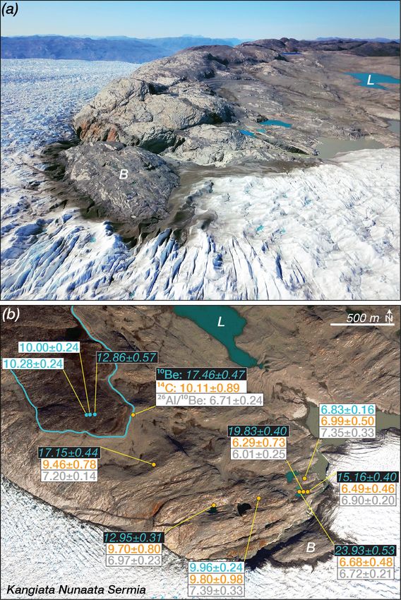
55 km north of KNS, and near Kangaasarsuup Sermia lo- Sediment cores from two proglacial–threshold lakes at Qa-
cated ∼ 20–25 km southwest of KNS (Lesnek et al., 2020; manaarsuup Sermia were collected using a universal percus-
Fig. 1). Moraine crests were mapped prior to fieldwork and sion corer and a Nesje-style percussion–piston coring de-
updated in the field. This mapping follows previous efforts vice (Fig. 3). Goose Feather Lake (informal name) is located
(Weidick, 1974; Weidick et al., 2012; Pearce et al., 2018), ∼ 2 km from the GrIS margin and currently receives GrIS
with the exception that we distinguish between early to mid- meltwater. We collected two piston cores at a water depth
dle Holocene moraines and moraines marking the GrIS his- of 12.60 m (17GOOF-A3 and 17GOOF-A4; 64.45328◦ N,
torical maximum extent (Figs. 2 and 3). Across the broader 49.44373◦ W). Marshall Lake (informal name) is located
KNS region, the distinction is obvious. Moraines and trim- ∼ 1 km from the GrIS margin and does not presently re-
lines attributed to the historical maximum extent of the GrIS ceive meltwater from the GrIS. We collected two cores from
are close to the modern ice margin and are fresh in appear- Marshall Lake with the universal percussion corer system
ance due to a lack of vegetation and lichen cover. Early at a water depth of 5.95 m (17MAR-A2 and 17MAR-C1;
Holocene moraines are typically located well outboard of the 64.46361◦ N 49.44373◦ W).
historical moraines and have extensive lichen cover. The key
exceptions to this spatial relationship are regions where ice
2.3 10 Be and 26 Al geochemistry and accelerator mass
is topographically confined near small outlet glaciers (Figs. 1
spectrometric measurements
and 3). In these locations, the historical maximum and early
Holocene moraines are closely stacked yet are still easily We completed 61 10 Be and 12 26 Al measurements; 54 of the
distinguishable based on their morphologies and degree of 10 Be samples and all of the 26 Al samples were processed
lichen cover (Figs. 3 and 4). at the Lamont–Doherty Earth Observatory (LDEO) cosmo-
Samples for cosmogenic nuclide analysis were collected genic dating laboratory (Tables S3, S4, and S5 in the Supple-
using a Hilti brand AG500-A18 angle grinder–circular saw ment). The remaining seven 10 Be samples were processed
with diamond bit blades, as well as a hammer and chisel. at the University at Buffalo Cosmogenic Isotope Laboratory
Clim. Past, 17, 419–450, 2021 https://doi.org/10.5194/cp-17-419-2021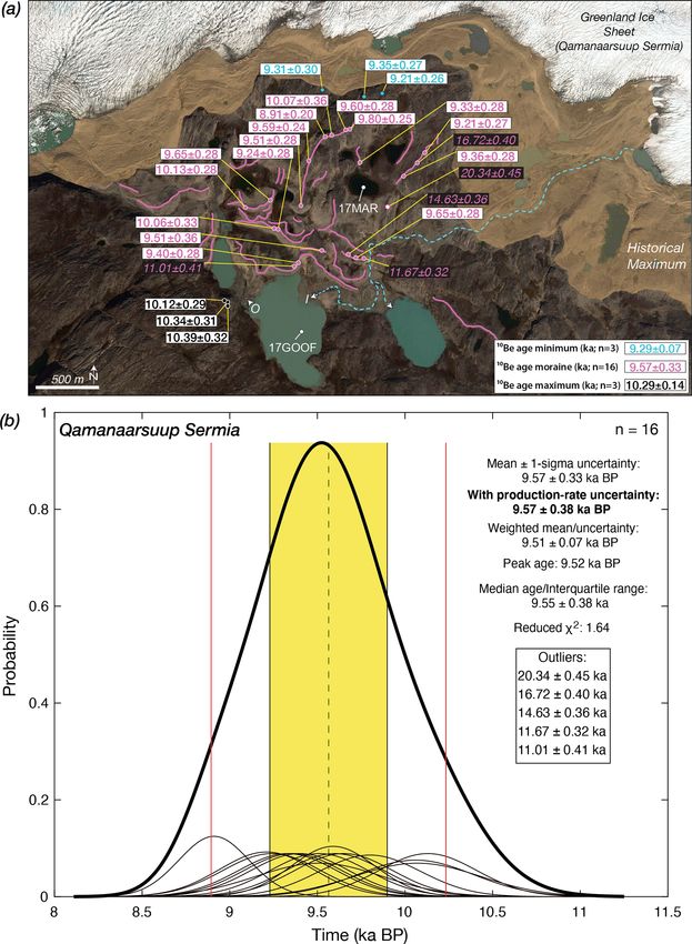
N. E. Young et al.: In situ cosmogenic 10 Be–14 C–26 Al measurements                                                                  423

Figure 3. (a) Qamanaarsuup Sermia region depicting the Kapisigdlit stade moraines (pink) and retreat since from the historical maximum
extent (brown shading); moraines were mapped in the field. 10 Be ages (ka ± 1 SD) are from three morphostratigraphic groups: (1) erratic
boulders perched on bedrock outboard of the Kapisigdlit stade moraines (black symbols and text), (2) Kapisigdlit stade moraine boulders
(pink symbols and text), and (3) erratic boulders perched on bedrock inside the Kapisigdlit stade moraines (blue symbols and text). 10 Be
ages influenced by isotopic inheritance are in italics with black boxes. Also shown are the sediment coring locations in Goose Feather Lake
(17GOOF) and Marshall Lake (17MAR). The dashed blue line marks the route of meltwater from the GrIS to the Goose Feather Lake inflow
(I). The outflow (O) for Goose Feather Lake routes meltwater back towards the GrIS. Map data: © Google Maps, Maxar Technologies. (b)
Normal density estimates for the Kapisigdlit stade moraines from panel (a). The age in bold includes the production-rate uncertainty.

(Tables S3 and S4). In both laboratories, quartz separation             27 Al was achieved (Table S5). Total 27 Al was quantified after

as well as Be and Al isolation followed well-established pro-           sample digestion using inductively coupled plasma optical
tocols (Schaefer et al., 2009). We quantified the amount of             emission spectrometry analysis of replicate aliquots. Accel-
native 27 Al in each quartz aliquot and then added varying              erator mass spectrometric analysis for 10 Be samples was split
amounts of 27 Al carrier to ensure that ∼ 1400–1750 mg of               between the Purdue Rare Isotope Measurement (PRIME)

https://doi.org/10.5194/cp-17-419-2021                                                                 Clim. Past, 17, 419–450, 2021
424                                                          N. E. Young et al.: In situ cosmogenic 10 Be–14 C–26 Al measurements

                                                                        of 2.7 % ± 0.5 % (n = 36; Table S3), and the 1σ analytical
                                                                        error for 26 Al measurements ranged from 1.9 % to 5.0 %
                                                                        with an average of 3.8 % ± 0.9 % (n = 12; Table S5). For
                                                                        10 Be samples measured at LLNL-CAMS, 1σ analytical error

                                                                        ranged from 1.6 % to 4.2 %, with an average of 2.3 %±0.8 %
                                                                        (n = 25; Table S3). Process blank corrections for all 10 Be and
                                                                        26 Al samples were applied by taking the batch-specific blank

                                                                        value (expressed as the number of atoms) and subtracting this
                                                                        value from the sample atom count (Tables S4 and S5). In ad-
                                                                        dition, we propagate through a 1.5 % uncertainty in the car-
                                                                        rier concentration when calculating 10 Be concentrations. We
                                                                        assume half-lives of 1.387 and 0.705 Ma for 10 Be and 26 Al
                                                                        (Chmeleff et al., 2010; Nishiizumi, 2004).

                                                                        2.4   In situ 14 C measurements
                                                                        We completed 12 in situ 14 C extractions at the LDEO cos-
                                                                        mogenic dating laboratory following well-established LDEO
                                                                        extraction procedures (Lamp et al. 2019; Table S6). All mea-
                                                                        sured fraction modern values are converted to 14 C concen-
                                                                        trations following Hippe and Lifton (2014). The LDEO in
                                                                        situ 14 C extraction laboratory has historically converted sam-
                                                                        ples to graphite prior to measurement by accelerator mass
                                                                        spectrometry and LLNL-CAMS; however, we have recently
                                                                        transitioned to gas-source measurements with the AixMI-
                                                                        CADAS instrument at CEREGE, which can directly mea-
                                                                        sure ∼ 10–100 µg C and largely removes the need for the
                                                                        addition of a carrier gas added to typical in situ 14 C sam-
                                                                        ples (Bard et al., 2015; Tuna et al., 2018). Here, two samples
                                                                        underwent traditional graphitization and were measured at
                                                                        LLNL-CAMS (Table S6), whereas the remaining 10 samples
                                                                        were measured with the CEREGE AixMICADAS instrument
Figure 4. (a) View to the northeast in the Qamanaarsuup Sermia          (Table S6). Both sets of samples underwent the same in situ
region (Fig. 3). In the foreground is a Kapisigdlit stade moraine       14 C extraction and 14 C sample gas clean-up procedures, with
crest resting directly adjacent to the historical maximum extent of
this sector of the GrIS (dashed line). The GrIS is in the background,
                                                                        only the samples measured at LLNL-CAMS undergoing an
and there has been minimal retreat from the historical maximum          additional graphitization procedure (Lamp et al., 2019). Be-
extent here. (b) View to the southwest in the Qamanaarsuup Sermia       cause we use two different measurement approaches and our
region showing Marshall Lake and Goose Feather Lake. Note the           extraction efforts span the transition between sample graphi-
color contrast between the two lakes. Marshall Lake currently does      tization and gas-source measurements, we briefly discuss our
not receive meltwater from the GrIS. Goose Feather Lake is cur-         data reduction methods for both sets of measurements (Ta-
rently a proglacial lake that receives silt-laden GrIS meltwater; the   ble S6).
lake catchment currently extends beneath the modern GrIS footprint         Samples 17GRO-14 and 17GRO-74 were measured at
(Figs. 3a and 6).                                                       LLNL-CAMS with 1σ analytical uncertainties of 2.2 % and
                                                                        3.0 % (Table S6). In situ 14 C concentrations were blank-
                                                                        corrected using a long-term mean blank value of 116 894 ±
Laboratory (n = 36) and the Center for Accelerator Mass                 37 307 14 C atoms with the uncertainty in the blank correction
Spectrometry at Lawrence Livermore National Laboratory                  propagated in quadrature (n = 27; updated from Lamp et al.,
(LLNL-CAMS; n = 25); all 26 Al samples were measured at                 2019). In addition, we propagate an additional 3.6 % uncer-
PRIME.                                                                  tainty in 14 C concentrations based on the long-term scatter in
   All 10 Be samples were measured relative to the 07KNSTD              internal graphite-based CRONUS-A standard measurements
standard with a 10 Be/9 Be ratio of 2.85 × 10⁻¹² (Nishiizumi            (698 109 ± 25 380 atoms g−1 ; n = 13; updated from Lamp
et al., 2007), and 26 Al samples were measured relative to the          et al., 2019); stated in situ 14 C concentrations for samples
KNSTD standard with the value of 1.82×10⁻¹² (Nishiizumi,                measured at LLNL-CAMS have total uncertainties of 7.7 %
2004). For 10 Be samples measured at PRIME, the 1σ an-                  and 10.4 %, respectively (Table S6).
alytical error ranged from 1.9 % to 3.9 % with an average

Clim. Past, 17, 419–450, 2021                                                               https://doi.org/10.5194/cp-17-419-2021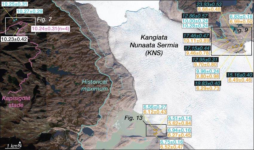
N. E. Young et al.: In situ cosmogenic 10 Be–14 C–26 Al measurements                                                              425

   Samples measured at CEREGE have 1σ analytical uncer-              lator found at https://hess.ess.washington.edu/ (last access:
tainties that range between 1.0 % and 2.8 % with a mean              27 August 2020), which implements an updated treatment of
of 1.4 % ± 0.5 % (n = 10; Table S6). For our gas-source              muon-based nuclide production (Balco et al., 2008; Balco,
measurements presented here and for future lab measure-              2017). We do not correct nuclide concentrations for snow
ments, we recharacterized our extraction and measurement             cover or subaerial surface erosion; samples are almost exclu-
procedure with a new set of process blank and CRONUS-A               sively from windswept locations, and many surfaces still re-
standard measurements (Table S6). We completed six pro-              tain primary glacial features. In addition, we make no correc-
cess blank gas-source measurements at CEREGE with val-               tion for the potential effects of isostatic rebound on nuclide
ues ranging from ∼ 73 000–175 000 14 C atoms (Table S6).             production because both the production-rate calibration sites
One blank measurement is anomalously high (174 813 ±                 and sites of unknown age have experienced similar exposure
3582 atoms; Table S6) and we suspect this blank was con-             and uplift histories (i.e., the correction is “built in”; Young
taminated by the atmosphere during collection in a break-            et al., 2020a, b). Individual 10 Be and in situ 14 C ages are pre-
seal. The remaining blank values have a mean of 85 768 ±             sented and discussed with 1σ analytical uncertainties, and
12 070 14 C atoms (n = 5), and we tentatively suggest that           moraine ages exclude the 10 Be production-rate uncertainty
removing the graphitization procedure may also remove a              when we compare them to other 10 Be-dated features. When
source of 14 C that was contributing to LDEO background              moraine ages are compared to independent records of cli-
14 C blank values. Here, we use running-mean blank val-              mate variability or ice-sheet change, the production-rate un-
ues of 81 094 ± 6972 (n = 4) and 85 768 ± 12 070 14 C atoms          certainty is propagated through in quadrature (1.8 %; Young
(n = 5) to correct sample 14 C concentrations and uncertain-         et al., 2013a). To allow for direct comparison to traditional
ties in the blank corrections are propagated in quadrature           radiocarbon constraints in the region, all 10 Be and in situ 14 C
(Table S6). In addition, we made five CRONUS-A standard              surface exposure ages are presented in thousands of years BP
measurements at CEREGE. Our CRONUS-A measurements                    (1950 CE); exposure ages relative to the year of sample col-
are remarkably consistent, with a mean value of 662 132 ±            lection can be found in the Supplement (2017 CE; Tables S3
9849 atoms g−1 (n = 5; 1.5 % uncertainty), and are compara-          and S6).
ble to our graphite-based value of 698 109±25 380 atoms g−1
(updated from Lamp et al., 2019). Nonetheless, despite the           2.6   Traditional 14 C ages from proglacial–threshold lakes
promising consistency of our gas-source CRONUS-A mea-
surements, we conservatively propagate through an addi-              Five radiocarbon ages from aquatic macrofossils were ob-
tional 3.6 % uncertainty in our sample concentrations based          tained from Marshall Lake (Figs. 3 and 4; Table S7 in
on the scatter in long-term LDEO CRONUS-A measure-                   the Supplement), and one radiocarbon age from an aquatic
ments. Total 14 C concentration uncertainties for samples            macrofossil was obtained from lake Kap01 (Fig. 1; Ta-
measured at CEREGE range from 4.3 % to 5.2 % with a mean             ble S7). In addition, we discuss two previously reported ra-
uncertainty of 4.6 % ± 0.2 % (Table S6).                             diocarbon ages from Goose Feather Lake, located adjacent
                                                                     to Marshall Lake (Lesnek et al., 2020; Table S7). Aquatic
                                                                     macrofossils were isolated from surrounding sediment us-
2.5 10 Be and in situ 14 C age calculations                          ing deionized water washes through sieves. Samples were
10 Be  and in situ 14 C surface exposure ages are calculated us-     freeze-dried and sent to the National Ocean Sciences Ac-
ing the Baffin Bay 10 Be production-rate calibration dataset         celerator Mass Spectrometry Facility (NOSAMS) at Woods
(Young et al., 2013a) and the West Greenland in situ 14 C            Hole Oceanographic Institution for age determinations. We
production-rate calibration dataset (Young et al., 2014). All        targeted aquatic macrofossils for dating because terrestrial
ages are presented using time-variant “Lm” scaling (Lal,             macrofossils may persist on the relatively low-energy Arc-
1991; Stone, 2000), which accounts for changes in the mag-           tic landscape for hundreds of years before washing into a
netic field, although these changes are minimal at this high         lake basin; dating terrestrial macrofossils could skew our
latitude (∼ 64◦ N); using “St” scaling, which does not ac-           interpretations. Hard-water effects on the 14 C ages, which
count for changes in the magnetic field, results in almost           could make age determinations erroneously old, are unlikely
identical ages (< 10 years) because the calibration sites are        in our study area because lake catchments are dominated by
all located at high latitudes. The 10 Be and in situ 14 C calibra-   Archean gneiss, and the study lakes are all well above local
tion datasets are both derived from sites in western Green-          marine limits. All new radiocarbon ages are calibrated us-
land with early Holocene exposure histories, and the in situ         ing CALIB 8.2 and the INTCAL20 dataset, and previously
14 C calibration measurements are derived from the same ge-          reported radiocarbon ages are recalibrated in the same man-
ologic samples as one of the 10 Be calibration sites (Young          ner using the INTCAL20 and MARINE20 datasets (Stuiver
et al., 2014). This combination of calibration datasets ensures      et al., 2020; Reimer et al., 2020; Heaton et al., 2020; Ta-
that the production rates and the 14 C/10 Be production ratio        bles S1 and S7).
are regionally constrained. All ages are calculated in MAT-
LAB using code from version 3 of the exposure age calcu-

https://doi.org/10.5194/cp-17-419-2021                                                              Clim. Past, 17, 419–450, 2021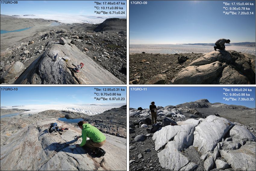
426                                                   N. E. Young et al.: In situ cosmogenic 10 Be–14 C–26 Al measurements

2.7   Ice-sheet model simulations of southwestern GrIS           temperature reconstructions due to uncertainty in the rela-
      change                                                     tionship between oxygen isotopes and surface air tempera-
                                                                 ture. Briner et al. (2020) pair three of the temperature recon-
We utilize recent paleo-simulations of southwestern GrIS         structions with each of the three precipitation reconstructions
change using the high-resolution Ice Sheet and Sea-level         to yield nine combinations that are used as transient climate
System Model (ISSM; Larour et al., 2012; Cuzzone et al.,         boundary conditions to force nine ice-sheet simulations. Two
2018, 2019; Briner et al., 2020). The model setup has been       of the five temperature reconstructions were not used because
previously described in Cuzzone et al. (2019) and Briner         they yield Younger Dryas ice-sheet margins that are inconsis-
et al. (2020), but here we briefly describe model attributes.    tent with geologic data.
The model domain extends from the present-day coastline             We use a positive degree day (PDD) method (Tarasov and
to the GrIS divide. The northern and southern boundaries of      Peltier, 1999) to compute the surface mass balance from tem-
the domain are far to the north and south of our study area.     perature and precipitation, and we use degree day factors of
The model resolution relies on anisotropic mesh adaptation       4.3 mm ◦ C−1 d−1 for snow and 8.3 mm ◦ C−1 d−1 for ice, with
to produce an unstructured mesh that varies based on bedrock     allocation for the formation of superimposed ice (Janssens
topography; bedrock topography is from BedMachine v3             and Huybrechts, 2000). We use a lapse rate of 6 ◦ C km−1
(Morlighem et al., 2017). For the southwestern GrIS, high        to adjust the temperature of the climate forcings to the ice-
horizontal model mesh resolution is necessary in areas of        surface elevation.
complex bed topography to prevent artificial ice-margin vari-
ability resulting from interaction with bedrock artifacts that
occur at coarser resolution (Cuzzone et al., 2019). Thus, the    3   Results
model mesh varies from 20 km in areas where gradients in
the bedrock topography are smooth to 2 km in areas where         Adjacent to Qamanaarsuup Sermia, 27 10 Be ages from
bedrock relief is high. In the KNS region the mesh varies        moraine boulders and boulders perched on bedrock range
from 2 to 8 km.                                                  from 20.34 ± 0.45 ka to 8.91 ± 0.20 ka (Figs. 3 and 5; Ta-
   The ice model applies a higher-order approximation (Blat-     ble S3). Sediments in Goose Feather Lake are composed of
ter 1995; Pattyn 2003) to solve the momentum balance             a lower gray silt unit overlain by organic sediments, which
equations and an enthalpy formulation (Ashwanden et al.,         is in turn overlain by gray silt (Lesnek et al., 2020). A sin-
2012), with geothermal heat flux from Shapiro and Ritz-          gle radiocarbon age from bulk sediments at the basal sedi-
woller (2004), to simulate the thermal evolution of the          ment contact is 8280 ± 90 cal yr BP, and a radiocarbon age
ice. Quadratic finite elements (P1 × P2) are used along the      from aquatic macrofossils at the upper contact between or-
z axis for the vertical interpolation, which allows the ice-     ganic and minerogenic sediments is 820 ± 80 cal yr BP. Sed-
sheet model to capture sharp thermal gradients near the bed,     iments in Marshall Lake display the same silt–organic–silt
while reducing computational costs associated with running       stratigraphy as sediments in Goose Feather Lake (Fig. 6).
a linear vertical interpolation with increased vertical layers   A radiocarbon age from aquatic macrofossils from the basal
(Cuzzone et al., 2018). Sub-element grounding-line migra-        sediment contact is 8720 ± 350 cal yr BP, and a radiocarbon
tion (Serrousi et al., 2013) is included in these simulations;   age from aquatic macrofossils at the uppermost contact is
however, due to prohibitive costs associated with running a      520±20 cal yr BP (Fig. 6). Three additional radiocarbon ages
higher-order ice model over paleoclimate timescales these        from aquatic macrofossils between the lowermost and upper-
simulations do not include calving parameterizations or any      most contacts are 7250±70, 3650±50, and 940±20 cal yr BP
submarine melting of floating ice.                               and are in stratigraphic order (Fig. 6).
   Nine ice-sheet simulations are forced with paleoclimate          In the KNS region, 27 10 Be ages from moraine boulders,
reconstructions from Badgeley et al. (2020), who used pa-        erratics perched on bedrock, and abraded bedrock surfaces
leoclimate data assimilation to merge information from pale-     range from 23.93 ± 0.53 to 5.38 ± 0.23 ka (Table S3), and 12
oclimate proxies and global climate models. The temperature      in situ 14 C ages from bedrock range from 10.11 ± 0.89 to
reconstructions rely on oxygen isotope records from eight        5.62 ± 0.84 ka (Table S6). In addition, 12 26 Al–10 Be ratios
ice cores; the precipitation reconstructions use accumulation    range from 7.35 ± 0.33 to 6.01 ± 0.25 (all bedrock). A sin-
records from five ice cores, and all are guided by spatial re-   gle radiocarbon age from aquatic macrofossils at the basal
lationships derived from the transient climate model simu-       contact between silt and organic sediments in lake Kap01 is
lation TraCE-21ka (Liu et al., 2009; He et al., 2013). The       9450 ± 440 cal yr BP (Fig. 1; Table S7).
climate reconstructions are shown to be in good agreement           North of Narsap Sermia near Caribou Lake (Fig. 1), three
with independent paleoclimate proxy data (Badgeley et al.,       10 Be ages from boulders perched on bedrock are 9.07±0.32,

2020, and references therein). Along with a main tempera-        8.66 ± 0.31, and 8.66 ± 0.31 ka (Fig. 1; Table S3). South
ture and precipitation reconstruction, Badgeley et al. (2020)    of KNS at Deception Lake, two 10 Be ages from boulders
provide two sensitivity precipitation reconstructions due to     perched on bedrock are 10.66 ± 0.34 and 9.52 ± 0.32 ka, and
uncertainty in the accumulation records and four sensitivity     near One-way lake, two 10 Be ages from boulders perched

Clim. Past, 17, 419–450, 2021                                                        https://doi.org/10.5194/cp-17-419-2021
N. E. Young et al.: In situ cosmogenic 10 Be–14 C–26 Al measurements 427
4 Deglaciation chronologies
4.1 Qamanaarsuup Sermia
A total of 27 10 Be ages from the Qamanaarsuup Sermia re-
gion range 20.34 ± 0.45 to 8.91 ± 0.20 ka (Figs. 3 and 5; Ta-
ble S3); however, the 10 Be ages are from three distinct mor-
phostratigraphic units. Here, the Kapisigdlit stade is marked
by numerous closely spaced moraine crests located immedi-
ately outboard of the historical moraines. Three 10 Be ages
from boulders resting on bedrock located outside the entire
Kapisigdlit moraine suite are 10.39±0.32, 10.34±0.31, and
10.12±0.29 ka, and they have a mean age of 10.29±0.14 ka,
which serves as a maximum-limiting age for the Kapisigdlit
stade moraines in the region. Three 10 Be ages from boulders
resting on bedrock immediately inboard of all Kapisigdlit
stade moraines, but outboard of the historical moraine, are
9.35 ± 0.27, 9.31 ± 0.30, and 9.21 ± 0.26 ka; they provide a
minimum-limiting age of 9.29 ± 0.07 ka (Fig. 3). Of the 21
10 Be ages from Kapisigdlit stade moraine boulders, 5 10 Be
ages are likely influenced by 10 Be inheritance as they are
older than the maximum-limiting 10 Be ages and similar in
age to deglacial constraints found ∼ 140 km west at the mod-
ern coastline (11.67±0.32 and 11.01±0.41 ka; Figs. 1 and 3;
Table S3), or they date to when the GrIS margin was likely
situated > 140 km to the west somewhere on the continen-
tal shelf (20.34 ± 0.45, 16.72 ± 0.40, and 14.63 ± 0.36 ka;
Figs. 1 and 3; Table S3). The remaining 16 10 Be ages from
the Kapisigdlit moraine set show no trend with distance from
the ice margin. These 10 Be ages overlap at 1σ uncertain-
ties with each other, the minimum-limiting 10 Be ages, or the
maximum-limiting 10 Be ages, suggesting that deposition of
this suite of moraine crests happened within dating resolu-
tion (i.e., we cannot resolve the ages of different moraine
crests). Combined, the 16 10 Be ages from moraine boul-
ders, excluding outliers, have a mean age of 9.57 ± 0.33 ka,
which is morphostratigraphically consistent with bracketing
maximum- and minimum-limiting 10 Be ages of 10.29 ± 0.14
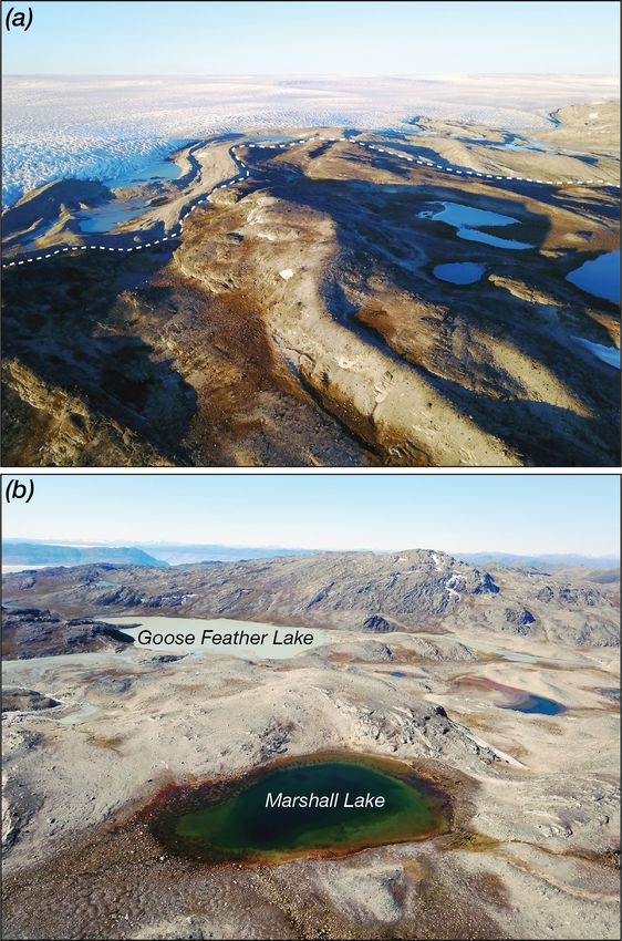
Figure 5. Representative boulder samples from the Qamanaar- and 9.29 ± 0.07 ka, respectively (Fig. 3). Including the un-
suup Sermia region (Fig. 3). Samples 17GRO-16, 17GRO-32, and
certainty in the 10 Be production-rate calibration, 10 Be ages
17GRO-39 are moraine boulder samples. 17GRO-25 is an erratic
from the Qamanaarsuup Sermia region reveal that the GrIS
boulder perched on bedrock inside the Kapisigdlit stade moraine
located only a few meters outboard of the historical maximum margin approached its modern extent at 10.29 ± 0.23 ka, de-
moraine, which can be seen in the background. Samples 17GRO- posited the Kapisigdlit stade moraines at 9.57 ± 0.38 ka, and
46 and 17GRO-47 are erratic boulders resting on bedrock located retreated behind the position of the historical maximum at
outboard of the Kapisigdlit stade moraine. 9.29 ± 0.18 ka.
Alternating silt–organic–silt sediment packages found in
Goose Feather and Marshall lakes are typical of those found
on bedrock are 16.43 ± 0.49 and 7.72 ± 0.26 ka (Fig. 1; Ta- in proglacial–threshold lakes in southwestern Greenland
ble S3). (Fig. 6; Briner et al., 2010; Larsen et al., 2015; Young and
Briner, 2015; Lesnek et al., 2020). Silt deposition occurs
when the GrIS margin resides within the lake catchment but
does not override the lake, feeding silt-laden meltwater into
the lake. Organic sedimentation occurs when the GrIS mar-
gin is not within the lake catchment and meltwater is diverted
elsewhere. Despite Goose Feather and Marshall lakes resid-
https://doi.org/10.5194/cp-17-419-2021 Clim. Past, 17, 419–450, 2021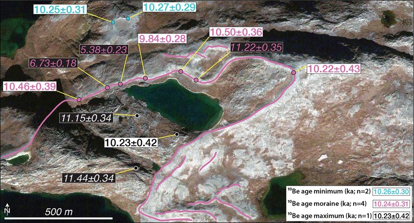
428                                                        N. E. Young et al.: In situ cosmogenic 10 Be–14 C–26 Al measurements

Figure 6. (a) Sediment cores and calibrated radiocarbon ages (±2σ ) from Marshall (MAR) and Goose Feather (GOOF) lakes. Note the
distinct color differences between silt and organic sediments (see Figs. 3 and 4). Details for radiocarbon ages can be found in Table S7. (b)
Sub-ice topography in the Qamanaarsuup Sermia region generated using the BedMachine v3 digital elevation model (Morlighem et al., 2017)
compared to our chronology of ice-margin change developed from 10 Be ages and radiocarbon-dated lake sediments (panel a). Shown is the
average 10 Be age from each feature on the landscape (including production-rate uncertainty; see Fig. 3) and basal radiocarbon ages from
panel (a). Deglaciation of the landscape just outboard of the Kapisigdlit stade moraines occurred at 10.29 ± 0.23 ka, followed by moraine
deposition at 9.57 ± 0.38 ka. Ice retreated behind the modern margin at 9.29 ± 0.18 ka, but the ice margin remained within the drainage
catchment of Goose Feather Lake until 8.28 ± 0.09 cal ka before retreating farther inland. The dashed line delimits the topographic threshold
(T) under the modern GrIS that the ice margin must cross in order for Goose Feather Lake to receive silt-laden meltwater. Inflow of meltwater
ceases when the GrIS margin retreats behind this topographic threshold, which rests ∼ 1 km behind the modern margin.

ing adjacent to each other on the landscape, their radiocarbon           and once ice thins below the valley edge, GrIS meltwater is
ages suggest slightly different ice-margin histories. Marshall           diverted elsewhere, likely indicating that the Goose Feather
Lake has a small and highly localized drainage catchment                 drainage divide resides near the modern ice margin (e.g.,
and does not receive GrIS meltwater at present. In contrast,             Young and Briner, 2015; Lesnek et al., 2020). Indeed, sub-
because Goose Feather Lake currently receives GrIS melt-                 ice topography in the Qamanaarsuup Sermia region reveals
water, its drainage catchment extends somewhere beneath                  that the topographic threshold dictating whether meltwater
the modern GrIS. Goose Feather Lake is fed by meltwater                  is diverted to Goose Feather Lake or elsewhere is located
sourced from an outlet glacier resting in an overdeepening,              within ∼ 1 km of the modern ice margin (Fig. 6). Despite the

Clim. Past, 17, 419–450, 2021                                                                  https://doi.org/10.5194/cp-17-419-2021
N. E. Young et al.: In situ cosmogenic 10 Be–14 C–26 Al measurements                                                         429

GrIS margin retreating behind the position of the historical      10.28 ± 0.24, and 10.00 ± 0.24 ka (Fig. 9). The 10 Be age of
maximum position at 9.29±0.18 ka, silt deposition in Goose        12.86 ± 0.57 ka is, again, almost certainly influenced by in-
Feather Lake until 8280 ± 90 cal yr BP indicates that the ice     heritance as this 10 Be age predates the timing of deglacia-
margin remained within ∼ 1 km of its present position be-         tion at the outer coastline. The remaining 10 Be ages of
tween ∼ 9.3 and 8.3 ka (Fig. 6).                                  10.28±0.24 and 10.00±0.24 ka are consistent with the 10 Be
                                                                  ages from inside the Kapisigdlit stade moraine (and outboard
4.2   Kangiata Nunaata Sermia
                                                                  of the historical maximum limit) on the west side of the fjord.
                                                                  Our new and previously published age constraints reveal that
A total of 15 10 Be ages in the KNS region constrain the          deposition of the Kapisigdlit stade moraine in the KNS fore-
timing of deposition of the Kapisigdlit stade moraines and        field occurred at ca. 10.4–10.2 ka, followed by retreat of the
the timing of when the GrIS retreated behind the eventual         GrIS within the historical maximum limit shortly thereafter
historical maximum limit (Figs. 2 and 7–9). West of the           (Fig. 2). Any possible moraine correlative with the ∼ 9.6 ka
KNS terminus, three 10 Be ages from erratic boulders perched      moraine found at Qamanaarsuup Sermia would have been
on bedrock located immediately outboard of the Kapisigdlit        overrun by the historical advance of KNS.
stade moraine are 11.44 ± 0.34, 11.15 ± 0.34, and 10.23 ±            Lastly, a basal minimum-limiting radiocarbon age of
0.42 ka. Seven 10 Be ages from moraine boulders range from        9450 ± 440 cal yr BP from Kap01 is, within uncertainties,
11.22 ± 0.35 to 5.38 ± 0.23 ka, and two 10 Be ages from er-       identical to a previously reported basal radiocarbon age of
ratic boulders perched on bedrock located immediately in-         9850 ± 290 cal yr BP from the same lake (Tables S1 and
side the moraine are 10.27±0.29 and 10.25±0.31 ka (Fig. 7).       S7; Larsen et al., 2014). We note that our new radiocar-
Deglaciation of the outer coast at Nuuk occurred at ∼ 11.2–       bon age is from aquatic macrofossils, whereas the previously
10.7 ka, suggesting that the single 10 Be age of 10.23±0.42 ka    published radiocarbon age is from bulk sediments (humic
from just outboard of the Kapisigdlit stade moraine is likely     acid extracts). Despite the risk of bulk sediments yielding
the closest maximum-limiting age on moraine deposition,           radiocarbon ages that are too old, basal radiocarbon ages
and 10 Be ages of 11.44 ± 0.34 and 11.15 ± 0.34 ka are likely     from Kap01 suggest that the offset between macrofossil-
influenced by a slight amount of inheritance (Figs. 1 and         and bulk-sediment-based radiocarbon ages is likely mini-
7). This maximum-limiting 10 Be age is consistent with a          mal during the initial onset of organic sedimentation follow-
maximum-limiting radiocarbon age of 10 170±340 cal yr BP          ing landscape deglaciation. We do not advocate for the use
from a bivalve reworked into Kapisigdlit stade till located       of bulk sediments to develop down-core chronologies, but
down-fjord (Weidick et al., 2012; Larsen et al., 2014; Fig. 1;    paired macrofossil–bulk sediment measurements from the
Table S1). The 10.23 ka age is also consistent with the 10 Be     same horizon often yield similar or indistinguishable radio-
age of boulders outboard of the Kapisigdlit stade moraines in     carbon ages in southwestern Greenland (e.g., Kaplan et al.,
the Qamanaarsuup Sermia study area of ∼ 10.29 ka. There is        2002; Young and Briner, 2015), suggesting that bulk sedi-
significant scatter in our moraine boulder 10 Be ages; the old-   ments will not produce significantly erroneous radiocarbon
est 10 Be age of 11.22 ± 0.35 ka is likely influenced by iso-     ages in this region. These similarities in southwestern Green-
topic inheritance, whereas the younger outliers of 6.73±0.18      land likely result from several factors: (1) a large fraction of
and 5.38 ± 0.23 ka reflect post-depositional boulder exhuma-      humic acid extracts are aquatic in origin (Wolfe et al., 2004);
tion (Fig. 7). The remaining 10 Be ages from the Kapisigdlit      (2) southwestern Greenland is composed almost entirely of
stade moraine have a mean age of 10.24 ± 0.31 ka (n = 4),         crystalline bedrock, thereby minimizing potential hard-water
which is supported by our minimum-limiting 10 Be ages of          effects; and (3) there is no significant accumulated carbon
10.27 ± 0.29 and 10.25 ± 0.31 ka from immediately inside          pool during the initial phase of ecosystem development (i.e.,
the moraine (Fig. 7). Indeed, 10 Be ages from erratic boulders    Wolfe et al., 2004). This latter point may be particularly in-
perched on bedrock located immediately inside moraines            fluential in southwestern Greenland because this region rests
across southwestern Greenland typically provide constraints       well inboard of the GrIS margin during glacial maxima (lo-
that are nearly identical to tightly clustered 10 Be ages from    cated on the continental shelf), resulting in a landscape that
moraine boulders (e.g., Young et al., 2011a, 2013b; Lesnek        is likely ice-covered for a significant fraction of each glacial
and Briner, 2018). Furthermore, our statistically identical       cycle. Furthermore, this sector of the GrIS is primarily warm-
10 Be ages from outboard and inboard of the Kapisigdlit stade     based and erosive, thereby further minimizing the likelihood
moraine, as well as from moraine boulders themselves, in-         of old carbon accumulating on the landscape at lower eleva-
dicate that moraine deposition occurred rapidly within the        tions.
resolution of our chronometer. Including the production-rate
uncertainty, we directly date the Kapisigdlit stade moraine to    4.3   Auxiliary sites
10.24 ± 0.36 ka, and all available supporting 10 Be and 14 C
ages further constrain moraine deposition to ∼ 10.4–10.2 ka.      At our site near Narsap Sermia, located ∼ 55 km north of
   On the east side of KNS, three 10 Be ages from immedi-         KNS, three 10 Be ages from boulders perched on bedrock
ately outboard of the historical maximum are 12.86 ± 0.57,        located outboard of the GrIS historical maximum and in-

https://doi.org/10.5194/cp-17-419-2021                                                          Clim. Past, 17, 419–450, 2021
430 N. E. Young et al.: In situ cosmogenic 10 Be–14 C–26 Al measurements Figure 7. Kapisigdlit stade moraine located just west of KNS (Fig. 2). 10 Be ages (ka ± 1 SD) are from three morphostratigraphic groups: (1) outboard of the moraine (black text and symbols), (2) moraine boulders (pink text and symbols), and (3) inside the moraine (blue text and symbols). 10 Be ages that are considered outliers are in black boxes with italics. Map data: © Google Maps, Maxar Technologies. Figure 8. Representative boulder samples related to the Kapisigdlit stade moraine west of KNS. 17GRO-64 and 17GRO-66 are moraine boulders, whereas 17GRO-67 and 17GRO-70 are erratic boulders resting on bedrock located immediately inboard and outboard of the Kapisigdlit stade moraine. board of the Kapisigdlit stade limit have a mean age of existing 10 Be and traditional 14 C age of 9.95 ± 0.19 ka (n = 8.80 ± 0.24 ka (8.80 ± 0.29 ka including the production-rate 2) and 8790 ± 190 cal yr BP from locations slightly more dis- uncertainty; Table S3), consistent with a minimum-limiting tal from the ice sheet suggest that our age of 10.66±0.34 ka is basal radiocarbon age of 7460 ± 110 cal yr BP (Lesnek et al., perhaps influenced by a small amount of isotopic inheritance 2020; Fig. 1; Table S1). Near Kangaasarsuup Sermia, located (Larsen et al., 2014; Fig. 1; Tables S2 and S3). The remaining ∼ 35 km south of KNS, two 10 Be ages from boulders perched age of 9.52 ± 0.32 ka is consistent with a minimum-limiting on bedrock outboard of the historical limit and inboard of the basal radiocarbon age of 9210 ± 190 cal yr BP from Decep- Kapisigdlit stade limit are 10.66±0.34 and 9.52±0.32 ka. An tion Lake (Fig. 1; Lesnek et al., 2020). Lastly, south of Kan- Clim. Past, 17, 419–450, 2021 https://doi.org/10.5194/cp-17-419-2021
N. E. Young et al.: In situ cosmogenic 10 Be–14 C–26 Al measurements                                                               431

                                                                        of early Holocene ice-margin change and historical observa-
                                                                        tions to quantify the maximum duration of Holocene expo-
                                                                        sure our bedrock samples sites could have experienced. First,
                                                                        we use 10 Be ages from immediately outboard of the historical
                                                                        limit on the northeastern side of KNS and 10 Be ages from just
                                                                        inboard of the Kapisigdlit stade moraine on the southwestern
                                                                        side of KNS to define the potential onset of Holocene ex-
                                                                        posure at our 10 Be–14 C–26 Al bedrock sites. 10 Be ages from
                                                                        outboard of the historical limit overlap at 1σ uncertainties
                                                                        (n = 4; excluding one outlier), and we calculate a mean age
                                                                        of 10.20 ± 0.14 ka (10.20 ± 0.23 ka with production-rate un-
                                                                        certainty) as the earliest onset of exposure at our inboard
                                                                        bedrock sites (Fig. 2). This age represents the timing of
                                                                        deglaciation immediately outboard of the historical limit and,
                                                                        assuming the continued retreat of the GrIS margin, the initial
                                                                        timing of exposure for the inboard bedrock sites (e.g., Young
                                                                        et al., 2016). Next, we capitalize on historical observations in
                                                                        the KNS region that constrain ice-margin change beginning
                                                                        in the 18th century (Weidick et al., 2012; Lea et al., 2014,
                                                                        and references therein). Based on scattered first-person ob-
                                                                        servations, the advance towards the eventual historical max-
                                                                        imum extent likely began by 1723–1729 CE and culminated
                                                                        in ca. 1750 CE, with initial ice-margin thinning taking place
                                                                        at ca. 1750–1800 CE (Weidick et al., 2012). Broadly sup-
                                                                        porting this record of ice-margin migration is an early pho-
                                                                        tograph by Danish geologist Hinrich Rink dated to sometime
                                                                        in the 1850s (Fig. 10). The photograph depicts the front of
                                                                        KNS as seen from the northwest and clearly delineates an
                                                                        existing historical maximum trimline, indicating that the lo-
                                                                        cal GrIS historical maximum was achieved and initial thin-
                                                                        ning from this maximum began prior to 1850 CE (Fig. 10;
Figure 9. (a) Oblique aerial view to the northwest depicting re-        Weidick et al., 2012). Additional first-person descriptions in-
cently deglaciated bedrock that rests between the historical maxi-      dicate that the KNS ice margin was more extended than to-
mum extent and the modern ice margin on the northeastern side of        day between ca. 1850 CE and at least 1948 CE, punctuated
KNS. (b) 10 Be and in situ 14 C ages (ka ± 1 SD), along with mea-       by the 1920 CE stade, which marks a significant readvance
sured 26 Al/10 Be ratios, at each bedrock sample site. 10 Be ages in-   of the ice margin (Fig. 2). Aerial photographs reveal that the
fluenced by inheritance are in black boxes with italics. The histori-   ice margin was only a few tens of meters east of our bedrock
cal maximum extent of KNS is marked in blue. To orient the reader,      sites on the western side of KNS at 1968 CE, suggesting site
L and B mark the same feature in each panel. Map data: © Google
                                                                        deglaciation shortly beforehand (Weidick et al., 2012). Our
Maps, Maxar Technologies.
                                                                        eastern ice-marginal bedrock sites were likely ice-free in ca.
                                                                        2000 CE based on satellite imagery.
                                                                           The majority of our bedrock sites are directly adjacent to
gaasarsuup Sermia near One-way Lake, two 10 Be ages from
                                                                        the ice margin, and we assume that pre-imagery historical
boulders perched on bedrock outboard of the historical limit
                                                                        observations of ice-margin change apply to both sampling
are 16.43 ± 0.49 and 7.72 ± 0.26 ka (Fig. 1; Table S3). The
                                                                        regions because any differences in ice-covered and ice-free
older of these two 10 Be ages is influenced by isotopic inheri-
                                                                        intervals between the two sampling sites are likely negligible
tance, leaving a single 10 Be age of 7.72 ± 0.26 ka as the only
                                                                        for our purposes. The available historical constraints indicate
estimate for the timing of local deglaciation.
                                                                        that our bedrock sites became ice-covered in ca. 1725 CE
                                                                        (historical maximum advance phase), and our sites on the
5   10 Be–14 C–26 Al    measurements from the KNS                       western side of KNS likely became ice-free in ca. 1968 CE;
    forefield                                                           ice-marginal sites on the east side of KNS became ice-free
                                                                        in ca. 2000 CE. These observations indicate that the west-
Prior to interpreting triple 10 Be–14 C–26 Al measurements in           ern bedrock sites experienced 243 years of historical ice
abraded bedrock located between the historical maximum                  cover, whereas the eastern sites experienced 275 years of
extent and the current ice margin, we use our new chronology            ice cover. With the earliest possible onset of exposure oc-

https://doi.org/10.5194/cp-17-419-2021                                                                Clim. Past, 17, 419–450, 2021
432 N. E. Young et al.: In situ cosmogenic 10 Be–14 C–26 Al measurements
of the well-constrained maximum possible exposure duration
provided by geologic constraints and historical observations,
here isotopic inheritance refers to exposure ages older than
10.20 ± 0.23 ka (i.e., pre-Holocene exposure).
5.1 Apparent in situ 10 Be and 14 C surface exposure
ages
Apparent 10 Be ages from abraded bedrock surfaces on the
northeastern side of KNS, listed from just inboard of the
historical maximum limit towards the modern ice margin,
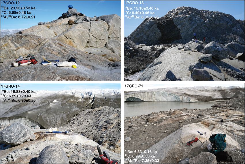
are 17.46 ± 0.47, 17.15 ± 0.44, 12.95 ± 0.31, 9.96 ± 0.24,
19.83 ± 0.40, 23.93 ± 0.53, 15.16 ± 0.40, and 6.83 ± 0.16 ka
(Figs. 2, 9, 11, and 12; Table S3). On the southwestern
side of KNS adjacent to the modern ice margin, 10 Be ages
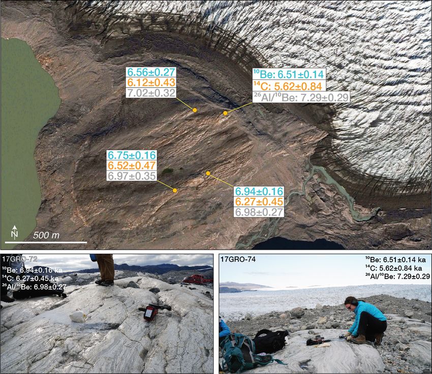
from abraded bedrock surfaces are 6.94 ± 0.16, 6.75 ± 0.16,
6.56 ± 0.27, and 6.51 ± 0.14 ka, all roughly at equal distance
from the present ice margin (Figs. 2 and 13; Table S3). Along
our northeastern transect, six of the eight apparent 10 Be ages
exceed the maximum allowable Holocene exposure duration
(10.20 ± 0.23 ka). Apparent 10 Be ages greater than this in-
dicate the presence of inherited 10 Be accumulated from a
period of pre-Holocene exposure and insufficient subglacial
erosion during the last glacial cycle to reset the cosmogenic
clock. Of the two remaining 10 Be ages not influenced by
isotopic inheritance, the 10 Be age of 9.96 ± 0.24 ka is sta-
tistically identical to the maximum allowable duration of
Holocene exposure for the landscape located between the
historical moraine and the modern ice margin. In addition,
Figure 10. (a) Photograph looking up-fjord towards KNS taken a 10 Be age of 6.83 ± 0.16 ka directly adjacent to the mod-
some time in the 1850s by Danish geologist Hinrich Rink (Weidick ern margin is suggestive of less exposure and more burial (or
et al., 2012). Our northeastern KNS field site (Fig. 9) is located on
more erosion; see Sect. 5.2) at this site, and it is also statisti-
the distal side of Nunaatarsuk. (b) Close-up of Akullersuaq (A) and
cally identical to apparent 10 Be ages from the southwestern
Nunaatarsuk (N) that captures the trimline marking the historical
maximum extent of KNS. The photograph is housed in the archives side of KNS, indicating similar Holocene exposure histories.
of the National Museum in Copenhagen. A digital copy was gra- Although the maximum amount of allowable Holocene
ciously provided by O. Bennike. exposure is well-constrained, we pair our 10 Be measure-
ments with in situ 14 C measurements to (1) further assess
the magnitude of isotopic inheritance in our bedrock samples
and (2) constrain post-10 ka fluctuations of the GrIS margin.
curring at 10.20 ± 0.23 ka as constrained by our 10 Be ages, Whereas long-lived nuclides such as 10 Be must be removed
we assume that the maximum duration of Holocene surface from the landscape via sufficient subglacial erosion, the rela-
exposure at all of our sites is 10.0 kyr. We do note, how- tively short half-life of 14 C (t1/2 = 5700 years) allows previ-
ever, that three of our bedrock sampling sites on the north- ously accumulated in situ 14 C to decay to undetectable lev-
eastern side of KNS are at a higher elevation and lie closer els after ∼ 30 kyr of simple burial of a surface by ice; with
to the historical maximum limit than the sites adjacent to the aid of subglacial erosion, in situ 14 C can reach unde-
the modern ice margin (Figs. 2 and 9). These high-elevation tectable levels more quickly. In contrast to our apparent 10 Be
sites almost certainly experienced shorter historical ice cover ages, which display varying degrees of Holocene exposure
than our lower-elevation ice-marginal sites, likely on the or- and isotopic inheritance, in situ 14 C measurements are con-
der of ∼ 150–200 years. But considering the uncertainties sistent with Holocene-only exposure histories. On the south-
in our chronology and analytical detection limits, we as- western side of KNS, four apparent in situ 14 C ages range
sume they have the same maximum Holocene exposure du- from 6.59±0.47 to 5.62±0.84 ka, and paired 10 Be–14 C mea-
ration of 10 kyr. Lastly, samples could inherit cosmogenic surements yield concordant exposure ages (Fig. 13). Within
nuclides from an earlier exposure (i.e., inheritance), and in our northeastern bedrock transect, the two highest-elevation
the strictest sense, the most recent period of exposure for our samples near the historical maximum limit with 10 Be ages of
bedrock sites equates to only the last few decades. Because 17.46 ± 0.47 and 17.15 ± 0.44 ka have significantly younger
Clim. Past, 17, 419–450, 2021 https://doi.org/10.5194/cp-17-419-2021You can also read