A new methodological framework for geophysical sensor combinations associated with machine learning algorithms to understand soil attributes
←
→
Page content transcription
If your browser does not render page correctly, please read the page content below
Geosci. Model Dev., 15, 1219–1246, 2022
https://doi.org/10.5194/gmd-15-1219-2022
© Author(s) 2022. This work is distributed under
the Creative Commons Attribution 4.0 License.

A new methodological framework for geophysical sensor
combinations associated with machine learning algorithms
to understand soil attributes
Danilo César de Mello1 , Gustavo Vieira Veloso1 , Marcos Guedes de Lana1 , Fellipe Alcantara de Oliveira Mello2 ,
Raul Roberto Poppiel2 , Diego Ribeiro Oquendo Cabrero3 , Luis Augusto Di Loreto Di Raimo4 ,
Carlos Ernesto Gonçalves Reynaud Schaefer1 , Elpídio Inácio Fernandes Filho1 , Emilson Pereira Leite4 , and
José Alexandre Melo Demattê2
1 Department  of Soil Science, Federal University of Viçosa, Viçosa, Brazil
2 Department  of Soil Science, Luiz de Queiroz College of Agriculture, University of São Paulo,
Av. Pádua Dias, 11, CP 9, Piracicaba, SP 13418-900, Brazil
3 Geography Department of Federal University of Mato Grosso do Sul, Av. Ranulpho Marques Leal, no. 3484,

Distrito Industrial CEP 79610-100 Três Lagoas/MS, Brazil
4 Department of Geology and Natural Resources, Institute of Geosciences, University of Campinas,

Rua Carlos Gomes, 250, Cidade Universitária, CEP 13083-855, Campinas/SP, Brazil

Correspondence: José Alexandre Melo Demattê (jamdemat@usp.br)

Received: 13 May 2021 – Discussion started: 16 July 2021
Revised: 13 December 2021 – Accepted: 16 December 2021 – Published: 10 February 2022

Abstract. Geophysical sensors combined with machine               collected data, without any sample preparation, for most of
learning algorithms were used to understand the pedosphere        the tested predictors (R 2 values ranging from 0.20 to 0.50).
system and landscape processes and to model soil attributes.      Also, the use of four regression algorithms proved to be im-
In this research, we used parent material, terrain attributes,    portant since at least one of the predictors used one of the
and data from geophysical sensors in different combinations       tested algorithms. The performance values of the best algo-
to test and compare different and novel machine learning al-      rithms for each predictor were higher than those obtained
gorithms to model soil attributes. We also analyzed the im-       with the use of a mean value for the entire area comparing the
portance of pedoenvironmental variables in predictive mod-        values of root mean square error (RMSE) and mean absolute
els. For that, we collected soil physicochemical and geo-         error (MAE). The best combination of sensors that reached
physical data (gamma-ray emission from uranium, thorium,          the highest model performance was that of the gamma-ray
and potassium; magnetic susceptibility and apparent elec-         spectrometer and the susceptibilimeter. The most important
tric conductivity) by three sensors (gamma-ray spectrome-         variables for most predictions were parent material, digital
ter, RS 230; susceptibilimeter KT10, Terraplus; and conduc-       elevation, standardized height, and magnetic susceptibility.
tivimeter, EM38 Geonics) at 75 points and analyzed the data.      We concluded that soil attributes can be efficiently modeled
The models with the best performance (R 2 0.48, 0.36, 0.44,       by geophysical data using machine learning techniques and
0.36, 0.25, and 0.31) varied for clay, sand, Fe2 O3 , TiO2 ,      geophysical sensor combinations. This approach can facili-
SiO2 , and cation exchange capacity prediction, respectively.     tate future soil mapping in a more time-efficient and envi-
Modeling with the selection of covariates at three phases         ronmentally friendly manner.
(variance close to zero, removal by correction, and removal
by importance) was adequate to increase the parsimony. The
results were validated using the method “nested leave-one-
out cross-validation”. The prediction of soil attributes by ma-
chine learning algorithms yielded adequate values for field-

Published by Copernicus Publications on behalf of the European Geosciences Union.

1220                                                                       D. Mello et. al.: A new methodological framework

1   Introduction                                                    Herrmann, 2019), soil texture (Taylor et al., 2018), miner-
                                                                    alogy (Wilford and Minty 2006; Barbuena et al. 2013), pH
The pedosphere is composed of soils and their connec-               (Wong and Harper, 1999), and organic carbon (Priori et al.,
tions with the hydrosphere, lithosphere, atmosphere, and bio-       2016).
sphere (Karpachevskii, 2011). Soils are the result of sev-             Soil magnetic susceptibility (κ) can be defined as the de-
eral processes and factors and their interactions, resulting        gree to which soil particles can be magnetized (Rochette et
in specific soil types or horizons. The main soil processes         al., 1992). The κ is related to several pedoenvironmental fac-
are weathering and pedogenesis (Breemen and Buurman,                tors, such as soil mineralogy, lithology, and geochemistry
2003; Schaetzl and Anderson, 2005), and the soil-forming            of ferrimagnetic secondary minerals, such as magnetite and
factors are parent material, relief, climate, organisms, and        maghemite (Ayoubi et al., 2018). Also, the κ parameter can
time (Jenny, 1994). Their interactions during soil genesis re-      be related to other soil secondary minerals, like ferrihydrite
sults in different soil attributes such as texture, mineralogy,     and hematite (Valaee et al., 2016). The great potential of this
color, structure, base saturation, and clay activity, among oth-    technique is related to geological studies (Shenggao, 2000;
ers.                                                                Correia et al., 2010), soil texture, and organic carbon stud-
   In recent decades, there has been a growing demand for           ies (Camargo et al., 2014; Jiménez et al., 2017), soil surveys
soil resource information worldwide (Amundson et al., 2015;         (Grimley et al., 2004), and pedogenesis and pedogeomorpho-
Montanarella et al., 2015). Soils are recognized as having          logical processes (Viana et al., 2006; Sarmast et al., 2017;
a key influence on global issues such as water availability,        Mello et al., 2020).
food security, sustainable energy, climate change, and envi-           Apparent electrical conductivity (ECa) is the ability of
ronmental degradation (Amundson et al., 2015; Pozza and             the soil to conduct an electrical current, expressed in mil-
Field, 2020). Therefore, understanding the role of spatial          lisiemens per meter. This soil property is related to the pres-
variations in surface and subsurface soil is fundamental for        ence/amount of solutes in the soil solution, whose concen-
its sustainable use as well as for other connected environ-         tration in 1 dS m−1 is equivalent to 10 meq L−1 (Richards,
mental resources and monitoring (Agbu et al., 1990). In this        1954). Concerning the geophysical methods, the ECa is a
sense, it is necessary to increase the acquisition of informa-      geotechnology for identifying the soil physicochemical at-
tion on the functional attributes of soils, and to achieve this,    tributes and their spatial variation (Corwin et al., 2003). Var-
relevant and reliable soil information, applicable from local       ious different soil attributes are related to the ECa, such as
to global scales, is required (Arrouays et al., 2014).              soil salinity (Narjary et al., 2019), soil texture (Domsch and
   The acquisition of soil data and their attributes is generally   Giebel, 2004), cation exchange capacity (Triantafilis et al.,
achieved by traditional soil survey techniques. However, new        2009), mineralogy, pore size distribution, temperature, and
geotechnologies have emerged in recent decades, allowing            soil moisture (McNeill, 1992; Rhoades et al., 1999; Bai et
the acquisition of data at shorter times, with non-invasive and     al., 2013; Farzamian et al., 2015; Cardoso and Dias, 2017).
accurate methods such as reflectance spectroscopy, satellite           As various sensors scan only the soil surface, disregard-
imagery, and geophysical techniques (Mello et al., 2020; De-        ing the entire soil tridimensional profile (Xu et al., 2019), a
mattê et al., 2017, 2007; Fioriob, 2013; Fongaro et al., 2018;      single sensor may not be able or be the best solution to quan-
Mello et al., 2021; Terra et al., 2018). Among these technolo-      tify multiple soil attributes. In this context, the concept and
gies, geophysical sensors have been recently used in pedol-         use of multi-sensor data acquisition and analysis is a comple-
ogy to understand pedogenesis and the relationship between          mentary way to offer more robust and accurate estimations
these processes and soil attributes (Son et al., 2010; Schuler      of a number of soil attributes (Xu et al., 2019; Javadi et al.,
et al., 2011; Beamish, 2013; McFadden and Scott, 2013; Sar-         2021). The analysis of soil data acquired by multiple sensors
mast et al., 2017; Reinhardt and Herrmann, 2019). Among             requires a careful interpretation and a mathematical model,
these geophysical techniques used, we highlight gamma-ray           which can be considered the base of the observed variation
spectrometry, magnetic susceptibility (κ), and apparent elec-       and provides the basis for generalization, prediction, and in-
trical conductivity (ECa).                                          terpretation (Heuvelink and Webster, 2001).
   Gamma-ray spectrometry can be defined as the measure-               Recently, many models have been used to estimate soil at-
ments of natural gamma radiation emission from natural              tributes and their spatial distribution from geophysical data
emitters, such as 40 K; the daughter radionuclides of 238 U         (gamma ray, κ, and ECa) and soil attributes, including ma-
and 232 Th; and total emissions from all elements in soils,         chine learning algorithms, such as the support vector ma-
rocks, and sediments (Minty, 1988). Weathering and pedo-            chine (SVM; Priori et al., 2014; Heggemann et al., 2017; Li
genesis, concomitantly with the geochemical behavior of             et al., 2017; Leng et al., 2018; Zare et al., 2020), random for-
each radionuclide, determine their distribution and concen-         est (Lacoste et al., 2011; Viscarra Rossel et al., 2014; Harris
tration in the pedosphere (Dickson and Scott, 1997; Wilford         and Grunsky, 2015; Sousa et al., 2020), KNN and artificial
and Minty, 2006; Mello et al., 2021). Therefore, gamma-ray          neural network (ANN) (Dragovic and Onjia, 2007), and Cu-
spectrometry can provide important information for the com-         bist (Wilford and Thomas, 2012) methods.
prehension of soil processes and attributes (Reinhardt and

Geosci. Model Dev., 15, 1219–1246, 2022                                             https://doi.org/10.5194/gmd-15-1219-2022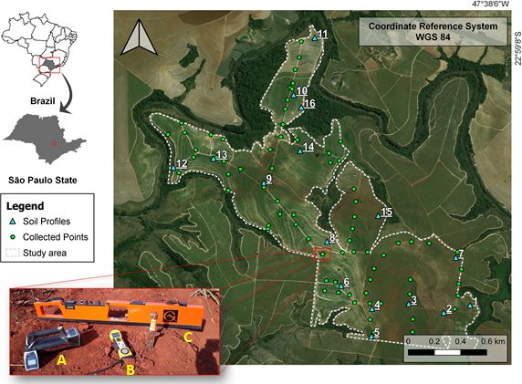
D. Mello et. al.: A new methodological framework 1221
According to Batty and Torrens (2001), the best models 22◦ 580 53.9700 S and 53◦ 390 47.8100 to 53◦ 370 25.6500 W), in
are those capable of explaining the same phenomena us- the Capivari River catchment, part of the Paulista Periph-
ing the smallest number of variables without loss of per- eric Depression geomorphological unit (Fig. 1). The lithol-
formance, following the principle of parsimony – Occam’s ogy is mainly composed of Paleozoic sedimentary rocks,
razor. Models that use fewer variables usually optimize the dominated by Itararé formation (siltites/meta-siltites) crossed
modeling process, making it easier to explain the influence by intrusive diabase dykes of the Serra Geral Formation.
of the variables on the modeling process and providing re- The lowlands are covered by Quaternary alluvial sediments
sults that are easier to interpret. In addition, this facilitates deposited by the Capivari River in ancient fluvial terraces
the understanding and the faster computer processing of the (Fig. 2a).
data (Brungard et al., 2015). In this context, the recursive fea- The heterogeneity of the landform and the parent materials
ture elimination (RFE) algorithm may be used for the back- drove the formation of several soil types (Fig. 2b). Previous
ward selection of optimal subsets of variables, while main- soil surveys and mapping have been performed in the study
taining a satisfactory model performance (Vašát et al., 2017; area by expert pedologists (Bazaglia Filho et al., 2013; Nanni
Hounkpatin et al., 2018). and Demattê, 2006), in which the main soil classes mapped
Some of geophysical sensors can detect soil attributes in were as follows: Cambisols, Phaeozems, Nitisols, Acrisols,
the upper soil layers (0–0.50 m for gamma-ray spectrometry and Lixisols (IUSS Working Group WRB, 2014). Besides the
by the RS230 model, 0.02 m for the magnetic susceptilimeter soil profiles, 75 subsamples from 75 points (0–20 cm layer)
KT10 Terraplus model, and 1.5 m for the conductivimeter via were collected with an auger for physicochemical analyses,
the EM38 model, for example), which are explained by nat- according to Fig. 1.
urally occurring soil processes and formation by soil factors According to the Köppen classification the region’s cli-
(Mello et al., 2020, 2021). However, there is still a knowledge mate is subtropical, mesothermal (Cwa), with an average
gap regarding the identification of the best covariables and temperature from 18 ◦ C (July–winter) to 22 ◦ C (February–
their possible combinations to deepen our knowledge of soil summer), and a mean annual precipitation between 1100 and
weathering, genesis, and their relation to soil attributes. A 1700 mm (Alvares et al., 2013).
standard approach to selecting the best input data to soil pre-
diction models has yet to be developed (Levi and Rasmussen,
2.2 Laboratory physicochemical analysis
2014), mainly for geophysical sensors, which are little used
in soil science. The identification of such covariates may im-
prove the understanding of the interplays between soil pro- For soil physical analyses, the soil samples were first air-
cesses and attributes, allowing an enhanced comprehension dried, ground, and sieved through a 2 mm mesh, followed by
of soils from the punctual to the landscape scale, supporting granulometric analysis. After that, clay, silt, and sand con-
digital soil mapping and better soil use and management. tents were determined by the densimeter method (Camargo
In this context, this study aimed to (i) develop a new et al., 1986). Using the granulometry data, the textural groups
methodological framework on modeling soil attributes us- were determined following the EMBRAPA (2011) method-
ing combined data from three different geophysical sensors ology.
at five different sensor combinations, (ii) assess the use of The exchangeable cations aluminum, calcium, and mag-
different machine learning algorithms and test the nested nesium (Al3+ , Ca2+ , and Mg2+ ) were determined using KCl
leave-one-out cross-validation (LOOCV) method for predic- solution (1 mol L−1 ) and quantified by titration (Teixeira et
tion and selection of suitable models for each soil attribute al., 2017). A Mehlich-1 solution was used to extract K+ ,
evaluated, and (iii) evaluate the results and the importance of which was quantified by flame photometry. Potential acidity
the variables and relate them to pedogeomorphological pro- (H+ + Al3 ) was determined using a calcium acetate solution
cesses. Our main hypothesis is that the combined use of three (0.5 mol L−1 ) at pH 7.0; for the pH in water determination,
geophysical sensor data enables a better prediction of soil the soil-to-solution ratio of 1 : 2.5 was used (Teixeira et al.,
attributes by different machine learning algorithms and bet- 2017). More details about the analysis methods can be found
ter model performance. This study can provide an important elsewhere (Teixeira et al., 2017). Soil organic carbon was
background for geoscience studies and the improvement of determined using the Walkley–Black method via oxidation
geophysical and soil survey procedures. with potassium (Teixeira et al., 2017; Pansu and Gautheyrou,
2006). The total iron content was determined using selective
dissolution in sulfuric acid (Teixeira et al., 2017; Lim and
2 Material and methods Jackson, 1983). The resulting extract was used to determine
the contents of silicon dioxide (SiO2 ) and titanium dioxide
2.1 Study area (TiO2 ), using the EMBRAPA methodology (2017). All other
chemical parameters, such as base sum (BS) cation exchange
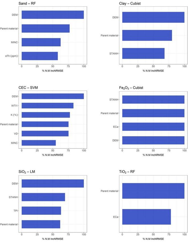
The study area was located on a sugarcane farm covering capacity (CEC), base saturation (V %), and aluminum satu-
184 ha, located in São Paulo state, Brazil (23◦ 00 31.3700 to ration (m %), were determined using the analytical data ob-
https://doi.org/10.5194/gmd-15-1219-2022 Geosci. Model Dev., 15, 1219–1246, 2022
1222                                                                           D. Mello et. al.: A new methodological framework

Figure 1. Study area, collection points, and geophysical sensors. A: gamma-ray spectrometer (Radiation Solution, RS 230);
B: susceptibilimeter (KT-10 Terraplus); C: Geonics Ground Conductivity Meter (EM 38).

tained previously, following the methodology described else-           ation Solutions, 2009). The measurements of radionuclides
where (Teixeira et al., 2017).                                         were taken in the “assay-mode” of the highest precision for
                                                                       quantification, in which the GM was kept at the soil sur-
2.2.1   Radionuclides and gamma-ray spectrometry data                  face for 2 min in each sampling point (79 total collection
                                                                       points) (Fig. 1). The geographic position was taken by a GPS
                                                                       coupled to the GM (GPS, Radiation Solution Inc., Ontario,
The total radionuclide 40 K amount was measured by the ab-
                                                                       Canada; precision of 1 m). The data collected from all points
sorption energy (1.46 MeV). Thorium (232 Th) and uranium
                                                                       were concatenated with their respective information from the
(238 U) were quantified by absorption energy (approximately
                                                                       soil physicochemical analyses for later geoprocessing. The
2.62 and 1.76 MeV, respectively). This quantification was
                                                                       same methodology has been applied by Mello et al. (2021)
indirectly performed through thallium (208 Tl) and bismuth
                                                                       for gamma-ray spectrometric data acquisition.
(214 Bi), derived by radioactive decay, respectively, for 232 Th
and 238 U, which are expressed as eTh and eU (equivalent
thorium and uranium, respectively).                                    2.2.2   Magnetic susceptibility (κ)
   For soil gamma spectrometric characterization, we used
the near-gamma-ray spectrometer (GM) model Radiation So-               For soil magnetic susceptibility (κ) characterization, surface
lution RS 230 (Radiation Solution Inc., Ontario, Canada)               readings were recorded at all 79 points, using a geophysi-
(Fig. 1a). The sensor can quantify the eTh and eU concen-              cal susceptibility meter sensor (KT10, Terraplus) (Fig. 1b).
trations in parts per million (ppm), whereas 40 K is quanti-           This sensor can measure κ to a depth of 2 cm below the soil
fied in percentage due to its major content in the pedosphere.         surface, with a precision of 10−6 in SI units, expressed in
Conventionally, radionuclides are expressed in mg kg−1 for             m3 kg−1 . To perform the readings, the sensor was first cali-
eU and eTh, whereas for 40 K, percentage is used. The GM               brated by determining the frequency of the outdoor oscilla-
detects the gamma-ray radiation emission down to a depth               tor. Subsequently, we followed the sequence required to ob-
of 30–60 cm, which varies mainly with soil bulk density and            tain the measurements performed in three steps: (1) deter-
moisture content (Wilford et al., 1997; Taylor et al., 2002;           mining the frequency and amplitude of the oscillator in free
Beamish, 2015).                                                        air; (2) measuring the frequency and amplitude of the oscil-
   First, the GM was automatically calibrated by switching             lator with the coil placed directly on the soil surface (sample)
on and leaving the sensor on the ground surface for 5 min              outcrop; and (3) repeating step 1 and displaying the results.
until readings of eU, eTh, and 40 K contents stabilized (Radi-         For more information about these procedures, see Sales, Sup-

Geosci. Model Dev., 15, 1219–1246, 2022                                                 https://doi.org/10.5194/gmd-15-1219-2022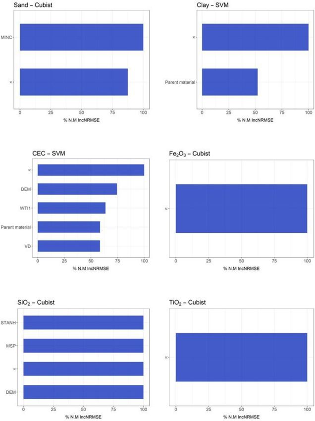
D. Mello et. al.: A new methodological framework                                                                              1223

Figure 2. (a) Geological compartments of the landscape. (b) Soil classes – CX: Haplic Cambisols, CY: Fluvic Cambisols, MT: Luvic
Phaozem, NV: Rhodic Nitisol: PA: Xanthic Acrisol, PVA: Rhodic Lixisol. The geological and soil class maps were adapted from Bazaglia
Filho et al. (2012). (c) Digital elevation model.

port and Cusomisation (2021). We performed the readings in          coil separation (Heil and Schmidhalter, 2019). More details
scanner mode, which uses the best geometric correlation to          about the EM38 operation are provided in Hendrickx and
direct κ readings, providing fast and accurate quantification.      Kachanoski (2002). After calibration, the ECa readings were
We performed three readings in triangulation around each            performed at all 75 collection points (Fig. 1), using the EM38
collection point and used the mean value of κ in all our anal-      at vertical dipole orientation, which provided data from an
yses. This procedure was adopted to reduce noise. The same          effective soil depth at 1.5 m. Data were collected in the field
methodology for κ readings has been performed by Mello et           during the dry season, on bare soil, and at the same inter-
al. (2020).                                                         vals to reduce the impacts of environmental variables. Also,
                                                                    all metal objects were kept away from the EM 38 to avoid
2.2.3   Apparent electrical conductivity (ECa)                      reading interferences.
                                                                       We developed our research and analysis by using three
The ECa measurements were performed using the conduc-               geophysical sensors (near-gamma-ray spectrometer RS 230,
tivity meter Geonics EM38 (Geonics Ltd., Mississauga, On-           near-magnetic susceptibility sensor KT10, and conduc-
tario, Canada) (McNeill, 1986) (Fig. 1c). The EM38 provides         tivimeter Geonics EM38) due to the following reasons: these
measurements of the quad-phase (conductivity) without any           sensors are available in our institution and for our research
requirement for soil-to-instrument contact (Geonics, 2002);         partners, they are easy to operate, and the obtained data are
the unit is m mS−1 .                                                highly accurate. In addition, the EM38 (conductivimeter) and
   First, the EM38 was calibrated following the instructions        RS 230 (gamma-ray spectrometer) provide information for
of Heil and Schmidhalter (2019), Sect. 3.1.1. The values            the depth at which most of the pedogenetic processes occur.
of ECa are a function of calibration, coil orientation, and

https://doi.org/10.5194/gmd-15-1219-2022                                               Geosci. Model Dev., 15, 1219–1246, 2022
1224                                                                      D. Mello et. al.: A new methodological framework

In addition, information obtained with EM38 and RS 230 can         performance of the machine learning algorithm will be the
be associated with KT10 (susceptibilimeter) on the soil sur-       mean performance indicators for all points (training/testing).
face to provide additional information about some soil at-         This is a robust method to evaluate the performance of the
tributes related to soil subsurface horizons, which is also re-    algorithm and to detect possible samples with problems in
lated to the other geophysical variables used (gamma-ray and       the collections or outliers. The training set generated in each
apparent electrical conductivity).                                 loop went through the process of selecting covariates for im-
                                                                   portance and subsequent training.
2.2.4   Modeling processing                                           The selection of covariates by importance is performed
                                                                   using the back forward method, applying the recursive fea-
The modeling process is demonstrated in the flowchart              ture elimination (RFE) function contained in the caret pack-
(Fig. 3) and can be divided into two parts: the selection of       age (Kuhn and Johnson, 2013). The RFE is unique for each
covariates and the training/testing of the data. In the selec-     algorithm, with the result being the set of selected covari-
tion phase, the algorithm tries to produce the ideal set of co-    ates used in the prediction of the final model in the same
variates, following the principle of parsimony. This is per-       algorithm. The RFE is a selection method that eliminates
formed by removing highly correlated variables, evaluating         the variables that least contribute to the model, based on
the importance of covariables, and removing variables that         a measure of importance for each algorithm (Kuhn and
have a minor importance in training the model in the predic-       Johnson, 2013). The algorithm will be applied to complete
tion process of each algorithm. Darst et al. (2018) considered     sets of data (variable by the set of tested sensors) and 18
the joint application of the methods for the selection of co-      more subsets with 5, 6, 7, . . . 19, 20, and 30 covariables.
variates by correlation and importance (RFE) since the use         Reaching a set of fewer variables (more parsimonious) re-
of RFE only reduces the effect of highly correlated covari-        sults in a better prediction performance. The optimization of
ates but does not eliminate it.                                    the ideal covariate subset was based on LOOCV, a repeti-
   The correlation selection process was used to calculate the     tion, and four values of each of the internal hype parame-
correlation of the set of covariates and covariables, which        ters of each tested algorithm (“tune length”). The hyperpa-
were evaluated with a correlation greater than the limit (Pear-    rameters of each algorithm are described in the caret pack-
son test > 95 %). The pairs that showed higher values were         age manual in chapter 6, “Models described”, available at
evaluated due to their correlation with the complete set of co-    https://topepo.github.io/caret/train-models-by-tag.html (last
variates, eliminating that with the highest value of the sum of    access: 1 February 2022). The metric for choosing the best
the absolute correlation with the other covariables that started   subset for each model was R 2 . For this work, five algorithms
in this process. For this phase, we applied the “cor” and          were tested: random forest (RF), Cubist (C), support vector
“find correlation” functions of the “stats” (Hothorn, 2021)        machines (SVMs), and generalized linear models (LMs). The
and “caret” (Kuhn et al., 2020) packages, in the R software,       choice was made with the use of families of different algo-
respectively (Kuhn and Johnson, 2013). In this phase, the co-      rithms in mind, using linear and non-linear algorithms. The
variables curv_cross_secational and curv_longitudinal were         algorithms used are commonly applied in soil attribute map-
eliminated for all tested sensor sets. The set of covariables      ping studies. At the end of the selection phase by importance,
that passed this phase joined the samples followed by the          the most optimized set of covariates for training was gener-
separation of samples from training and testing.                   ated for each algorithm.
   The separation of training and testing was performed               Training was performed with the variables selected in the
using the “nested” leave-one-out (nested-LOOCV) method             previous step and each tested algorithm by using LOOCV
(Clevers et al., 2007; Honeyborne et al., 2016; Rytky et           and 10 repetitions. Four values of each of the internal hype
al., 2020). It is important to highlight that the number of        parameters of each tested algorithm were also tested (tune
soil samples and readings with geophysical sensors was             length). At the end of the training phase, a sample prediction
small (75) due to several difficulties encountered in the field    was made that was not used in the training, and the result
during data collection (high sugar cane size, sloping terrain,     was saved for the performance study. The performance of
dense forest, etc.). In this sense, the nested LOOCV method        the prediction of the algorithms and the set of sensors was
is indicated for small sample sets (values near 100 samples)       determined with a set of samples from the outer loop of the
to which other validation/testing methods (such as holdout         nested-LOOCV method. Three evaluation parameters were
validation) would not be viable due to the small sample set        used: R squared, R 2 (Eq. 1); root mean squared error, RMSE
in the testing and/or training group (Ferreira et al., 2021).      (Eq. 2); mean absolute error, MAE (Eq. 3).
This is one of the main innovations of this research.                       P                             2
   The nested LOOCV method is a double-loop process. In                         Qpred − Qpred × Qobs − Qobs
                                                                   R 2 = hP                                     2 i ,        (1)
the first loop, the model is trained with a data set of size                  Qpred − Qpred
                                                                                            2 i hP
                                                                                                 ×  Qobs − Qobs
n − 1, and the test is done in the second loop with the miss-
ing sample to validate the training performance (Jung et al.,
2020; Neogi and Dauwels, 2022). The final results of the

Geosci. Model Dev., 15, 1219–1246, 2022                                            https://doi.org/10.5194/gmd-15-1219-2022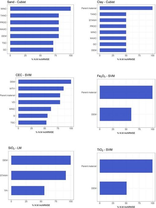
D. Mello et. al.: A new methodological framework                                                                                           1225

Table 1. Terrain variables generated from the digital elevation model.

              Terrain attributes                                Abbreviations   Brief description
              Convergence index                                 CI              Convergence/divergence index in relation to runoff
              Cross-sectional curvature                         CSC             Measures the curvature perpendicular to the
                                                                                downslope direction
              Flow-line curvature                               FLC             Represents the projection of a gradient line to a hori-
                                                                                zontal plane
              General curvature                                 GC              Combination of both plan and profile curvatures
              Hill                                              HI              Analytical hill shading
              Hill index                                        HIINDEX         Analytical index hill shading
              Longitudinal curvature                            LC              Measures the curvature in the downslope direction
              Mass balance index                                MBI             Balance index between erosion and deposition
              Maximal curvature                                 MAXC            Maximum curvature in local normal section
              Mid-slope position                                MSP             Represents the distance from the top to the valley,
                                                                                ranging from 0 to 1
              Minimal curvature                                 MINC            Minimum curvature for local normal section
              Multiresolution index of     ridge top flatness   MRRTF           Indicates flat positions in high-elevation areas
              Multiresolution index of valley bottom flatness   MRVBF           Indicates flat surfaces at the bottom of the valley
              Normalized height                                 NH              Vertical distance between base and ridge of normal-
                                                                                ized slope
              Plan curvature                                    PLANC           Curvature of the hypothetical contour line passing
                                                                                through a specific cell
              Profile curvature                                 PROC            Surface curvature in the direction of the steepest
                                                                                incline
              Slope                                             S               Represents local angular slope
              Slope height                                      SH              Vertical distance between base and ridge of slope
              Standardized height                               STANH           Vertical distance between base and standardized slope
                                                                                index
              Surface specific points                           SSP             Indicates differences among specific surface shift
                                                                                points
              Tangential curvature                              TANC            Measured in the normal plane in a direction perpen-
                                                                                dicular to the gradient
              Terrain ruggedness index                          TRI             Quantitative index of topography heterogeneity
              Terrain surface convexity                         TSC             Ratio of the number of cells that have positive curva-
                                                                                ture to the number of all valid cells within a specified
                                                                                search radius
              Terrain surface texture                           TST             Splits surface texture into 8, 12, or 16 classes
              Total curvature                                   TC              General measure of surface curvature
              Topographic position index                        TPI             Difference between a point elevation to the surround-
                                                                                ing elevation
              Valley depth                                      VD              Calculation of vertical distance at drainage base level
              Valley                                            VA              Calculation of the fuzzy valley using the top-hat ap-
                                                                                proach
              Valley index                                      VAI             Calculation of the fuzzy valley index using the top-hat
                                                                                approach
              Topographic wetness index                         TWI             Describes the tendency of each cell to accumulate wa-
                                                                                ter in relief

https://doi.org/10.5194/gmd-15-1219-2022                                                            Geosci. Model Dev., 15, 1219–1246, 2022
1226 D. Mello et. al.: A new methodological framework
Figure 3. Methodological flowchart showing the sequence of methodologies applied for soil and geophysical attribute prediction. The most
accurate model among Cubist, random forest (RF), support vector machines (SVMs), and linear models (LMs) was selected to model and
map the geophysical and soil attributes.
where Qpred denotes predicted samples, Qobs denotes ob-
r served samples, and n denotes the number of samples.
1 X 2 For comparison purposes, null model values
RMSE = × Qobs − Qpred , (2)
n (NULL_RMSE and NULL_MAE) were also calcu-
1 X lated. The null model considers using the average value
MAE = × Qpred − Qobs , (3)
n quantified by the collected samples (Eqs. 4 and 5). The null
model (NULL_RMSE and NULL_MAE) emulates other
Geosci. Model Dev., 15, 1219–1246, 2022 https://doi.org/10.5194/gmd-15-1219-2022D. Mello et. al.: A new methodological framework 1227
model-building functions but returns the simplest model lected particular groups of terrain attributes for the modeling
possible given a training set: a single mean for numeric of each soil attribute (Table 1).
outcomes. The percentage of the training set samples with The Cubist algorithm (non-use of the geophysical sensor)
the most prevalent class is returned when class probabilities showed the best performance in predicting soil texture, clay
are requested. The null model can be considered the simplest (R 2 of 0.386), and sand (R 2 of 0.292) contents, with the high-
model that can be adjusted and that serves as a reference. est R 2 and the lowest RMSE and MAE values, concomitantly
Models that present similar or worse performances com- (Table 2). The importance of covariates to sand content pre-
pared to the null model should be discarded. The best diction showed that minimal curvature was the most impor-
models had lower RMSE and MAE results than those found tant variable, contributing 100 % to the decrease mean accu-
for NULL_MAE and NULL_RMSE. This shows that the racy. On the other hand, for clay content, the most impor-
final model is better than using the mean values, which also tant variable was parent material. In addition, for clay and
demonstrates a better quality in creating the models. sand, the tangential curvature and DEM showed an impor-
Given the above, the null model considers using the mean tance higher than 50 % (Fig. 4).
value quantified by the collected samples (Eqs. 4 and 5). This When the geophysical sensor was not used, the SVM
methodology is widely used, as well as spatialization pro- algorithm presented a moderate performance for Fe2 O3
cesses in kriging when the variable in which spatialization (R 2 0.279) and TiO2 (R 2 0.226), whereas for SiO2 , the LM
is desired has spatial dependence (pure nugget effect). The presented the best result, also with a moderate performance
equations are as follows: (R 2 0.247) (Table 2). The selected models simultaneously
1 presented the highest R 2 and lowest RMSE and MAE val-
1 XN 2 2 ues. The most important covariates for Fe2 O3 and TiO2 pre-
NULL_RMSE = Qtrain i − Qobsi , (4)
N i=1 diction by the SVM model were parent material (100 %) and
1 X DEM (more than 50 %). For SiO2 prediction by the LM, the
NULL_MAE = × Qtrain i − Qobsi , (5) most important covariates were DEM (100 %) and standard-
n
ized height (90 %), whereas parent material contributed 40 %
where Qtrain denotes the mean of the training samples, Qobsi (Fig. 4).
denotes the validation sample, N denotes the number of sam- For cation exchange capacity (CEC), the model with the
ples (loop). best performance after 75 runs was SVM (R 2 of 0.223) (Ta-
Here NULL_RMSE and NULL_MAE values lower than ble 2) when the geophysical sensor was not used. The most
those observed in the prediction of the algorithm in the val- important covariates for CEC prediction to mean accuracy
idation phase show that the use of means of the samples of were DEM (100 %), topographic wetness index (80 %), and
the desired propriety agrees with the model created by the parent material (75 %) (Fig. 4).
algorithms of the machine learning. The NULL_RMSE and All models showed a low performance in the prediction
NULL_MAE were calculated using the “null mode” function of base saturation (BS) and organic matter (OM), with R 2
of the caret package (Kuhn et al., 2020). values between 0.001 and 0.1 (Tables 2–6).
The final result of the performance of the algorithms of The different combinations of geophysical sensors
each attribute was obtained using the 75 loops, with the train- that contributed to the moderate modeling performance
ing results being the average of the performance and the for soil attributes were as follows: susceptibilime-
results of the test samples calculated from the 75 external ter + conductivimeter (S + C), gamma-ray spectrome-
loops results using Eqs. (1)–(3). The importance of the algo- ter + conductivimeter (G + C), and combined use of the
rithms was calculated by the caret package (Kuhn and John- three geophysical sensors (G + S + C) (Tables 3, 4, and
son, 2013); each model presents its creation methodology. 6, respectively). The R 2 values presented some variations
The final importance for each algorithm and attribute was between the R 2 of the best combination of geophysical
determined from the importance created in the loop, being sensors and the lowest R 2 values when the geophysical
the average of the importance of the 75 repetitions. sensors were not used in the predictive models (Tables 3,
4, and 6). Among all the values of R 2 evaluated for this
3 Results session, we considered all the highest values; among the
highest values, we considered the lowest values as the worst
3.1 Geophysical sensor combinations, model results.
performance, uncertainty, and covariate For clay, the model with the best performance was the
importance SVM algorithm (R 2 0.484) using S + C (Table 3), whereas
that with the worst performance was the Cubist algorithm
The worst performance in modeling soil attributes occurred (R 2 0.38) using G + S + C (Table 6). For sand, the best
excluding the use of geophysical sensors (non-use of the geo- model performance was obtained with the Cubist algo-
physical sensor), where only parent material and terrain at- rithm (R 2 0.365) using S + C (Table 3) and the worst also
tributes were used (Table 2). In this case, the algorithms se- by Cubist (R 2 0.387) using G + S + C. The most impor-
https://doi.org/10.5194/gmd-15-1219-2022 Geosci. Model Dev., 15, 1219–1246, 20221228 D. Mello et. al.: A new methodological framework
Table 2. Model performance for non-use geophysical sensors, for all soil attributes, based on R 2 , RMSE, MAE, and NULL_RMSE.
R2
Non-use of geophysical sensors
Random forest Cubist SVM LM –
Clay 0.38 0.386 0.259 0.285 –
Sand 0.284 0.292 0.278 0.225 –
Fe2 O3 0.159 0.12 0.279 0.217 –
TiO2 0.12 0.125 0.226 0.16 –
SiO2 0.12 0.174 0.128 0.247 –
CEC 0.149 0.053 0.195 0.002 –
BS 0.131 0.028 0.113 0.003 –
OM 0 0.001 0.004 0.051 –
RMSE
Non-use of geophysical sensors
Random forest Cubist SVM LM NULL_RMSE
Clay 136.778 140.103 154.406 156.646 140.885
Sand 185.398 192.867 190.151 215.355 176.521
Fe2 O3 61.686 66.432 59.453 66.357 53.341
TiO2 12.229 12.424 11.621 13.118 10.239
SiO2 41.701 41.323 42.595 38.976 35.45
CEC 41.3 50.065 41.141 997.529 36.139
BS 20.206 22.853 20.396 1189.64 17.142
OM 8.469 8.126 8.045 7.702 6.158
MAE
Non-use of geophysical sensors
Random forest Cubist SVM LM NULL_MAE
Clay 110.485 108.284 122.397 119.139 119.751
Sand 149.205 148.8 147.07 169.218 153.803
Fe2 O3 40.742 44.028 36.812 43.673 41.578
TiO2 8.206 8.294 7.051 8.749 8.074
SiO2 31.757 31.715 31.432 29.458 29.534
CEC 28.931 33.168 27.072 149.114 27.187
BS 16.3 18.271 17.012 158.638 14.425
OM 6.357 4.813 5.992 5.719 4.813
CEC: cation exchange capacity; SVM: support vector machine; LM: linear model; BS: base saturation; OM: organic matter. Clay and
sand content in g kg−1 ; Fe2 O3 , TiO2 , and SiO2 in g kg−1 ; CEC in mmolc dm−3 , OM in g dm−3 ; BS in mmolc dm−3 .
tant covariates for clay prediction by the SVM model in the to TiO2 , the best model performance was by the Cubist algo-
S + C sensor combination were magnetic susceptibility (κ) rithm (R 2 0.358) using G + S + C (Table 6) and the worst
(100 %) and parent material (90 %) (Fig. 5). For clay pre- was RF (R 2 0.248) using G + C (Table 4). For SiO2 , the best
diction by the Cubist model in the G + S + C sensor com- model performance was the Cubist algorithm (R 2 0.250) us-
bination, the most important covariate was parent material ing S + C (Table 3) and the worst was the LM (R 2 0.178)
(100 %) (Fig. 6). With respect to sand prediction, the most using G + C (Table 4). The importance of covariates in pre-
important covariates by the Cubist model in S + C were dicting Fe2 O3 by LM in G + S + C demonstrated that mag-
minimal curvature (100 %) and magnetic susceptibility (κ) netic susceptibility (κ), standardized height, and DEM were
(80 %) (Fig. 5). On the other hand, for G + S + C, the co- the most important variables, contributing 100 %, 65 %, and
variates that most contributed to sand prediction were DEM 55 %, respectively (Fig. 6). For Fe2 O3 predicted by the Cu-
(100 %), general curvature (80 %), and minimal curvature bist algorithm using G + C, the most important covariates
(75 %) (Fig. 6). were standardized height, parent material, ECa, and DEM
For the elemental composition, the models employed (100 %) (Fig. 7). For TiO2 prediction by the Cubist algorithm
greatly variable performance. For Fe2 O3 the best model per- using G + S + C the most important covariate was magnetic
formance was reached by the LM algorithm (R 2 0.441) using susceptibility (κ) (100 %) (Fig. 6), while for the RF algorithm
G + S + C (Table 6), while the worst performance was by using G + C, they were parent material (100 %) and ECa
the Cubist (R 2 0.282) using G + C (Table 4). With respect (75 %) (Fig. 7). In relation to SiO2 prediction by the Cubist
Geosci. Model Dev., 15, 1219–1246, 2022 https://doi.org/10.5194/gmd-15-1219-2022D. Mello et. al.: A new methodological framework 1229 Figure 4. Variable importance for non-use of geophysical sensors (only variables that contributed more than 50 % are presented here). For further details, see Supplement. using S + C, the most important covariates were standard- In relation to CEC, the LM algorithm was the best model ized height, mid-slope position magnetic susceptibility (κ), (R 2 0.317) using G + S + C (Table 6) and the worst was and DEM (100 %) (Fig. 5), while those for SiO2 predicted the SVM algorithm (R 2 0.223) using S + C (Table 3). The by the LM algorithm using G + C were DEM and standard- most important covariate for prediction of CEC by the LM ized height (100 % and 65 %, respectively) to mean accuracy algorithm using G + S + C and using S + C was magnetic (Fig. 7). susceptibility (κ) (100 %) (Figs. 5 and 6). https://doi.org/10.5194/gmd-15-1219-2022 Geosci. Model Dev., 15, 1219–1246, 2022
1230                                                                                           D. Mello et. al.: A new methodological framework

Table 3. Model performance for the combined use of susceptibilimeter and the conductivimeter, for all soil attributes, based on R 2 , RMSE,
MAE, and NULL_RMSE.

                        Susceptibilimeter +                                                     R2
                        conductivimeter              Random forest            Cubist         SVM                LM                       –
                        Clay                                    0.444          0.433         0.484           0.394                       –
                        Sand                                    0.334          0.365         0.322           0.312                       –
                        Fe2 O3                                  0.314          0.407         0.153           0.383                       –
                        TiO2                                    0.316          0.338         0.263           0.262                       –
                        SiO2                                    0.141           0.25         0.169           0.101                       –
                        CEC                                     0.139          0.178         0.223           0.124                       –
                        BS                                      0.138          0.079         0.065           0.002                       –
                        OM                                      0.032          0.077         0.039           0.056                       –
                        Susceptibilimeter +                                                 RMSE
                        conductivimeter              Random forest            Cubist         SVM                LM       NULL_RMSE
                        Clay                                 129.619        136.834       127.598         139.463                140.885
                        Sand                                  178.22        178.253       181.811         190.515                176.521
                        Fe2 O3                                55.378         52.416        64.573           54.36                 53.341
                        TiO2                                  10.531         10.583        11.052          11.622                 10.239
                        SiO2                                  41.116         39.138         42.22          46.013                  35.45
                        CEC                                   41.878          41.91        40.134           48.52                 36.139
                        BS                                    19.821         21.543        22.307        1219.091                 17.142
                        OM                                     8.079          7.494         7.924           8.007                  6.158
                        Susceptibilimeter +                                                  MAE
                        conductivimeter              Random forest            Cubist         SVM                LM        NULL_MAE
                        Clay                                 102.841         105.12        92.812         106.083                119.751
                        Sand                                 145.441        139.737       146.016         153.815                153.803
                        Fe2 O3                                34.357         32.246        40.303           36.79                 41.578
                        TiO2                                   6.457          6.593          6.65           8.199                  8.074
                        SiO2                                   30.54         28.954        31.153          33.218                 29.534
                        CEC                                   29.354         28.912        26.689          33.024                 27.187
                        BS                                    15.824         17.372        18.953         161.284                 14.425
                        OM                                     5.949          5.713         6.108            6.04                  4.813
                      CEC: cation exchange capacity; SVM: support vector machine; LM: linear model; BS: base saturation; OM: organic
                      matter. Clay and sand content in g kg−1 ; Fe2 O3 , TiO2 , and SiO2 in g kg−1 ; CEC in mmolc dm−3 , OM in g dm−3 ; BS in
                      mmolc dm−3 .

   Overall, the best combination of geophysical sensors,                             whereas for SiO2 , the Cubist algorithm was the most suit-
which allowed the best model performance for different al-                           able (R 2 0.207), also using G + S (Table 5). The most im-
gorithms in the prediction of soil attributes, was gamma-ray                         portant covariates for Fe2 O3 and TiO2 prediction via LM us-
spectrometer + susceptibilimeter (G + S) (Table 5).                                  ing G + S were magnetic susceptibility (κ) and standardized
   For soil texture, the SVM and RF algorithms showed the                            height (100 % and 60%, respectively, for both) (Fig. 8). For
best performance for clay (R 2 0.494) and sand (R 2 0.422),                          SiO2 prediction via the Cubist algorithm using G + S, the
respectively, using G + S, with the highest R 2 and lowest                           most important covariates were mid-slope position and mag-
RMSE and MAE values (Table 5). The importance of covari-                             netic susceptibility (κ) (100 % for both) (Fig. 8).
ates in predicting soil texture by the SVM (for clay) and the                           For CEC, the best model performance was obtained using
RF (for sand) demonstrated that magnetic susceptibility (κ)                          the LM algorithm (R 2 0.303) using G + S (Table 5). In this
was the most important covariate (100 %). In addition, parent                        case, the covariates that most contributed to model prediction
material contributed 60 % for clay prediction and DEM 60 %                           were magnetic susceptibility (κ) (100 %) and DEM (60 %)
for sand prediction (Fig. 8).                                                        (Fig. 8).
   The LM algorithm presented the best performance for
Fe2 O3 (R 2 0.470) and TiO2 (R 2 0.328), using G + S,

Geosci. Model Dev., 15, 1219–1246, 2022                                                                    https://doi.org/10.5194/gmd-15-1219-2022
D. Mello et. al.: A new methodological framework 1231
Table 4. Model performance for the combined use of gamma-ray spectrometer and the conductivimeter, for all soil attributes based on R 2 ,
RMSE, MAE, and NULL_RMSE.
Gamma-ray spectrometer + R2
conductivimeter Random forest Cubist SVM LM –
Clay 0.378 0.433 0.406 0.338 –
Sand 0.318 0.265 0.3 0.188 –
Fe2 O3 0.22 0.282 0.158 0.249 –
TiO2 0.248 0.189 0.048 0.171 –
SiO2 0.16 0.163 0.17 0.178 –
CEC 0.14 0.077 0.241 0.002 –
BS 0.133 0.065 0.068 0.003 –
OM 0.001 0 0.059 0.047 –
Gamma-ray spectrometer + RMSE
conductivimeter Random forest Cubist SVM LM NULL_RMSE
Clay 137.097 134.231 134.035 146.116 140.885
Sand 179.808 197.657 182.644 225.909 176.521
Fe2 O3 58.829 56.918 61.758 62.442 53.341
TiO2 11.011 12.026 13.076 13.035 10.239
SiO2 40.256 42.209 40.493 41.555 35.45
CEC 41.464 47.809 40.463 1499.11 36.139
BS 19.889 21.704 21.586 33.64 17.142
OM 8.567 8.356 7.72 7.738 6.158
Gamma-ray spectrometer + MAE
conductivimeter Random forest Cubist SVM LM NULL_MAE
Clay 108.636 105.954 106.779 117.816 119.751
Sand 145.511 160.722 148.469 181.07 153.803
Fe2 O3 38.867 37.335 39.185 42.121 41.578
TiO2 7.265 8.241 8.197 9.198 8.074
SiO2 31.095 32.419 32.189 32.035 29.534
CEC 28.539 33.06 26.449 207.159 27.187
BS 15.812 17.471 17.325 24.294 14.425
OM 6.443 6.07 5.578 5.806 4.813
CEC: cation exchange capacity; SVM: support vector machine; LM: linear model; BS: base saturation; OM: organic matter. Clay
and sand content in g kg−1 ; Fe2 O3 , TiO2 , and SiO2 in g kg−1 ; CEC in mmolc dm−3 , OM in g dm−3 ; BS in mmolc dm−3 .
4 Discussion of soil by the Cubist algorithm and obtained the worst results
without using the sensors. Most likely, this is a result of the
4.1 Geophysical sensor combinations, models highly complex interaction between soil forming factors and
performance, and uncertainty processes determining soil attributes (Jenny, 1994).
The moderate performance of the models can be attributed
to the different combinations of the geophysical sensors pair-
The methodological approach optimized the prediction of
wise, and the different data presented by the sensors con-
soil variables by applying different geophysical sensor com-
tributed in different ways to the modeling process. In this
binations, parent material, and terrain attributes for selecting
regard, O’Rourke et al. (2016) also demonstrated a moderate
covariates and models, as well as for assessing prediction un-
performance of the models (R 2 ranging from 0.21 to 0.94)
certainty.
when using data from the Vis-NIR, with R 2 ranging from
In general, without the use of geophysical sensors, the
0.61 to 0.94 when using the pXRF sensor to model soil at-
poorest results were obtained in terms of R 2 , RMSE, and
tributes. This might be related to the different sensors and
MAE for all prediction algorithms used for modeling soil
their relation with soil attributes. The Vis-NIR spectroscopy
attributes (Table 2). These results are consistent with Frihy
acts on targets with low energy levels, showing the ability to
et al. (1995), who also compared the combined use and the
identify soil mineral species, strongly linked to soil attributes
non-use of sensors regarding model geochemical attributes
https://doi.org/10.5194/gmd-15-1219-2022 Geosci. Model Dev., 15, 1219–1246, 20221232 D. Mello et. al.: A new methodological framework Figure 5. Variable importance for susceptibilimeter + conductivimeter sensors (only variables that contributed more than 50 % are presented here; for further details see Supplement). (Coblinski et al., 2021). In addition, pXRF spectroscopy al- pXRF with Vis-NIR data for obtaining information about soil lows the identification of total elementary contents by act- constituents is highly efficient for modeling soil attributes. ing with high levels of ionizing energy, which is not identi- The best combination of geophysical sensors was gamma- fied by Vis-NIR and is strongly correlated with minerals and ray spectrometer + susceptibilimeter (G + S), with the high- soil attributes (Silvero et al., 2020). Therefore, the addition of est values of R 2 and the lowest values of RMSE and Geosci. Model Dev., 15, 1219–1246, 2022 https://doi.org/10.5194/gmd-15-1219-2022
D. Mello et. al.: A new methodological framework                                                                                  1233

Figure 6. Variable importance for combined use of the three geophysical sensors (only variables that contributed more than 50 % are pre-
sented here; for further details see Supplement).

MAE (Table 5). Most likely, the gamma-ray spectrometer                tion to thorium, uranium, and potassium (40 K) levels as well
and the susceptibilimeter are more closely associated with            as magnetic susceptibility.
pedogenesis (argilluviation, ferralitization, and others), pe-           In general, the Cubist algorithm was the best model for
dogeomorphology, and soil attributes, as recently demon-              clay and sand content prediction (Table 7). Similar results
strated by Mello et al. (2020, 2021), who modeled soil at-            have been found by Greve and Malone (2013); Ballabio et
tributes such as texture, Fe2 O3 , TiO2 , SiO2 , and CEC in rela-     al. (2016); Nawar et al. (2016); and Silva et al. (2019), who

https://doi.org/10.5194/gmd-15-1219-2022                                                 Geosci. Model Dev., 15, 1219–1246, 2022
1234                                                                         D. Mello et. al.: A new methodological framework

Figure 7. Variable importance for gamma-ray spectrometer + conductivimeter sensors (only variables that contributed more than 50 % are
presented here; for further details see Supplement).

used the Cubist and Earth algorithm to predict soil texture us-      the data set, causing poor modeling prediction. Zhang and
ing different data sources (3D imagery, Land Use and Cov-            Hartemink (2020) state that textural classes with fewer sam-
erage Area frame Survey, and reflectance spectroscopy). In           ples presented a more unstable prediction performance than
all these models, the R 2 was not greater than 0.5, which can        those with more samples, which agrees with our results.
be explained by the small variation or limited distribution of

Geosci. Model Dev., 15, 1219–1246, 2022                                               https://doi.org/10.5194/gmd-15-1219-2022
D. Mello et. al.: A new methodological framework                                                                                                1235

Table 5. Model performance for combined use of gamma-ray spectrometer and susceptibilimeter, for all soil attributes, based on R 2 , RMSE,
MAE, and NULL_RMSE.

                    Gamma-ray spectrometer +                                                        R2
                    susceptibilimeter                     Random forest           Cubist         SVM             LM                       –
                    Clay                                             0.465         0.441         0.494         0.366                      –
                    Sand                                             0.422         0.152         0.367         0.233                      –
                    Fe2 O3                                            0.36         0.426         0.096          0.47                      –
                    TiO2                                             0.308         0.282         0.284         0.328                      –
                    SiO2                                             0.159         0.207         0.169         0.167                      –
                    CEC                                              0.147         0.152         0.296         0.303                      –
                    BS                                               0.169         0.082         0.112         0.002                      –
                    OM                                               0.046         0.033         0.028         0.034                      –
                    Gamma-ray spectrometer +                                                   RMSE
                    susceptibilimeter                     Random forest           Cubist         SVM             LM       NULL_RMSE
                    Clay                                          127.149       132.977        123.84        148.11               140.885
                    Sand                                          165.624       244.635        175.35       202.104               176.521
                    Fe2 O3                                         53.418        52.737        67.759        48.513                53.341
                    TiO2                                           10.724         11.37        10.846        10.659                10.239
                    SiO2                                           40.898        40.244        42.207        42.993                 35.45
                    CEC                                            41.902        44.296        38.723        37.645                36.139
                    BS                                             19.294        21.318        20.856       1024.32                17.142
                    OM                                                 7.8        7.842          7.81         8.131                 6.158
                    Gamma-ray spectrometer +                                                     MAE
                    susceptibilimeter                     Random forest           Cubist         SVM             LM        NULL_MAE
                    Clay                                          102.229       105.123        97.173       117.097               119.751
                    Sand                                          134.525       168.957       140.318       166.083               153.803
                    Fe2 O3                                         33.284        32.411        42.282        33.124                41.578
                    TiO2                                            6.548         6.573         6.447         7.049                 8.074
                    SiO2                                           30.394        29.691        30.396        32.951                29.534
                    CEC                                            28.977        30.945        25.376        25.815                27.187
                    BS                                             15.597        17.321         16.96       137.422                14.425
                    OM                                              5.805         5.836         5.966         6.262                 4.813
                  CEC: cation exchange capacity; SVM: support vector machine; LM: linear model; BS: base saturation; OM: organic matter. Clay
                  and sand content in g kg−1 ; Fe2 O3 , TiO2 , and SiO2 in g kg−1 ; CEC in mmolc dm−3 , OM in g dm−3 ; BS in mmolc dm−3 .

   The better performance for elemental composition                                This is related to the high complexity of soils, such as the
(Fe2 O3 , TiO2 , and SiO2 ) was obtained using the Cubist al-                      high spatial variability in surface and depth; the occurrence
gorithm (Table 7), with an R 2 of 0.2–0.47. This is contrast-                      of geomorphic processes, weathering, and pedogenesis; and
ing with the results obtained by Henrique et al. (2018), who                       the different soil formation factors. For soil mineralogical at-
showed that the best model for predicting soil mineralogy                          tributes predicted by machine learning algorithms, the results
Fe2 O3 and TiO2 (R 2 0.89 and 0.96, respectively) and RF                           can be classified as satisfactory from 0.2 to 0.5, as for the
only for Fe2 O3 (R 2 0.95) by pXRF was the simple linear                           preliminary evaluation, since these values represent more in-
regression. In our study, the R 2 variation for the G + S com-                     formative results (Beckett, 1971; Dobos, 2003; Malone et al.,
bination was probably related to the low correlation with the                      2009). According to Nanni and Demattê (2006), the R 2 may
parent material and, consequently, with soil mineralogy or                         be explained by standardized laboratory conditions (such as
to the limited number of samples and the high soil variabil-                       temperature, humidity, substance concentrations, and other
ity (Fiorio, 2013). However, it is important to highlight that                     variables that interfere with the analysis results during their
in situ, various intrinsic environmental influences can inter-                     determination), with less environmental interference com-
fere with modeling processes. For example, the relatively low                      pared with direct field methods.
R 2 values (approximately between 0.2 and 0.5) can be at-                             For CEC, the best model performance was obtained for
tributed to the difficulty in modeling soils and their attributes.                 SVM (R 2 0.296) (Table 5). This result is corroborated by

https://doi.org/10.5194/gmd-15-1219-2022                                                                   Geosci. Model Dev., 15, 1219–1246, 2022
1236 D. Mello et. al.: A new methodological framework
Table 6. Model performance for all combined use of geophysical sensors, for all soil attributes, based on R 2 , RMSE, MAE, and
NULL_RMSE.
Combined use of the three R2
geophysical sensors Random forest Cubist SVM LM –
Clay 0.356 0.387 0.331 0.258 –
Sand 0.318 0.322 0.278 0.129 –
Fe2 O3 0.281 0.406 0.309 0.441 –
TiO2 0.322 0.358 0.267 0.252 –
SiO2 0.162 0.212 0.21 0.125 –
CEC 0.171 0.266 0.246 0.317 –
BS 0.122 0.097 0.107 0.002 –
OM 0.003 0.073 0.002 0.047 –
Combined use of the three RMSE
geophysical sensors Random forest Cubist SVM LM NULL_RMSE
Clay 139.61 139.41 144.532 160.894 140.885
Sand 180.339 188.745 189.768 256.078 176.521
Fe2 O3 57.225 52.66 57.589 50.038 53.341
TiO2 10.472 10.547 11.053 11.499 10.239
SiO2 40.642 40.534 40.355 43.949 35.45
CEC 41.451 39.226 39.815 37.134 36.139
BS 19.951 21.749 21.178 1045.896 17.142
OM 8.234 7.569 8.134 7.752 6.158
Combined use of the three MAE
geophysical sensors Random forest Cubist SVM LM NULL_MAE
Clay 112.126 108.346 117.645 120.83 119.751
Sand 143.98 145.661 145.187 198.059 153.803
Fe2 O3 35.597 32.751 35.387 34.724 41.578
TiO2 6.414 6.541 6.7 8.102 8.074
SiO2 30.215 30.197 30.001 33.649 29.534
CEC 29.014 27.169 26.201 25.273 27.187
BS 15.887 17.694 17.025 140.716 14.425
OM 6.223 5.854 5.945 5.798 4.813
CEC: cation exchange capacity; SVM: support vector machine; LM: linear model; BS: base saturation; OM: organic matter. Clay
and sand content in g kg−1 ; Fe2 O3 , TiO2 , and SiO2 in g kg−1 ; CEC in mmolc dm−3 , OM in g dm−3 ; BS in mmolc dm−3 .
Liao et al. (2014), who compared the model performance of and 0.50 can be considered satisfactory and reliable (Dobos,
multiple stepwise regression, artificial neural network mod- 2003; Malone et al., 2009). In our study, the low R 2 values
els, and SVM for CEC prediction and attributed their results can be related to the limited number of collecting points or to
to a nonlinear relationship between CEC and soil physico- the low field distribution, which does not represent the spatial
chemical properties. In addition, in our previous study (Ja- variation of soil attributes; this is in agreement with Johnston
farzadeh et al., 2016), we demonstrated that, despite the abil- et al. (1997) and Lesch et al. (1992), who evaluated soil salin-
ity of SVM to predict CEC in acceptable limits, there is a ity.
poor performance in extrapolating the maximum and min- The best results for predictors of soil attributes through
imum values of CEC data. Despite this, uncertainties esti- geophysical data have the lowest values when compared to
mated for SVM predictions may not be associated with an in- the values of NULL_RMSE and NULL_MAE. This demon-
correct classification, as pointed out by Cracknell and Read- strates that the use of machine learning models has less errors
ing (2013). than the use of mean values for the entire area (Table 5), re-
Even for the best combination of sensors (G + S) and the sulting in a better performance and accuracy.
highest overall model performance, the R 2 values were not The null model is a simple model (naive) that expresses the
greater than 0.5 (Table 5). In models generated by field data, value of the mean of the Y (variable to be predicted or tar-
without sample preparation, R 2 values varying between 0.20 get variable). The RMSE and MAE values are calculated for
Geosci. Model Dev., 15, 1219–1246, 2022 https://doi.org/10.5194/gmd-15-1219-2022You can also read