Modeling study of the impact of SO2 volcanic passive emissions on the tropospheric sulfur budget - Recent
←
→
Page content transcription
If your browser does not render page correctly, please read the page content below
Atmos. Chem. Phys., 21, 11379–11404, 2021
https://doi.org/10.5194/acp-21-11379-2021
© Author(s) 2021. This work is distributed under
the Creative Commons Attribution 4.0 License.

Modeling study of the impact of SO2 volcanic passive emissions on
the tropospheric sulfur budget
Claire Lamotte1 , Jonathan Guth1 , Virginie Marécal1 , Martin Cussac1 , Paul David Hamer2 , Nicolas Theys3 , and
Philipp Schneider2
1 CNRM,   Université de Toulouse, Météo-France, CNRS, Toulouse, France
2 NILU  – Norwegian Institute for Air Research, P.O. Box 100, 2027 Kjeller, Norway
3 Royal Belgian Institute for Space Aeronomy, BIRA-IASB, Brussels, Belgium

Correspondence: Claire Lamotte (claire.lamotte@meteo.fr)

Received: 6 October 2020 – Discussion started: 12 October 2020
Revised: 25 May 2021 – Accepted: 17 June 2021 – Published: 28 July 2021

Abstract. Well constrained volcanic emissions inventories in      canic SO2 emissions represent 15 % of the total annual sul-
chemistry transport models are necessary to study the im-         fur emissions, the volcanic contribution to the tropospheric
pacts induced by these sources on the tropospheric sulfur         sulfate aerosol burden is 25 %, which is due to the higher al-
composition and on sulfur species concentrations and deposi-      titude of emissions from volcanoes. Moreover, a sensitivity
tions at the surface. In this paper, the changes induced by the   study on passive degassing emissions, using the annual un-
update of the volcanic sulfur emissions inventory are stud-       certainties of emissions per volcano, also confirmed the non-
ied using the global chemistry transport model MOCAGE             linear link between tropospheric sulfur species content with
(MOdèle de Chimie Atmosphérique à Grande Échelle). Un-            respect to volcanic SO2 emissions. This study highlights the
like the previous inventory (Andres and Kasgnoc, 1998), the       need for accurate estimates of volcanic sources in chemistry
updated one (Carn et al., 2016, 2017) uses more accurate in-      transport models in order to properly simulate tropospheric
formation and includes contributions from both passive de-        sulfur species.
gassing and eruptive emissions. Eruptions are provided as
daily total amounts of sulfur dioxide (SO2 ) emitted by vol-
canoes in the Carn et al. (2016, 2017) inventories, and de-
gassing emissions are provided as annual averages with the        1   Introduction
related mean annual uncertainties of those emissions by vol-
cano. Information on plume altitudes is also available and has    Sulfur emissions come mainly from human activities (fos-
been used in the model. We chose to analyze the year 2013,        sil fuel combustion) and volcanic activity (Andreae, 1985).
for which only a negligible amount of eruptive volcanic SO2       Among them, sulfur dioxide (SO2 ) is a pollutant species
emissions is reported, allowing us to focus the study on the      known to affect both human health and the environment.
impact of passive degassing emissions on the tropospheric         Because of their link to the formation of acid rain and sul-
sulfur budget. An evaluation against the Ozone Monitoring         fate aerosols which can induce climate forcing (Chestnut,
Instrument (OMI) SO2 total column and MODIS (Moderate-            1995; Robock, 2000, 2007; Smith et al., 2001; Schmidt et al.,
Resolution Imaging Spectroradiometer) aerosol optical depth       2012; Kremser et al., 2016), SO2 emissions became a ma-
(AOD) observations shows the improvements of the model            jor concern in environmental policies. In some regions of
results with the updated inventory. Because the global vol-       the world, these policies led to strong reductions in anthro-
canic SO2 flux changes from 13 Tg yr−1 in Andres and Kas-         pogenic SO2 emissions in recent decades (Fioletov et al.,
gnoc (1998) to 23.6 Tg yr−1 in Carn et al. (2016, 2017), sig-     2016; Krotkov et al., 2016; Aas et al., 2019). Over North
nificant differences appear in the global sulfur budget, mainly   America and Europe, emissions strongly decreased between
in the free troposphere and in the tropics. Even though vol-      2005 and 2015. In the East Asia region, the decrease only
                                                                  happened after 2010 (Sun et al., 2018). In contrast, over In-

Published by Copernicus Publications on behalf of the European Geosciences Union.
11380            C. Lamotte et al.: Modeling study of the impact of volcanic emissions on the tropospheric sulfur budget

dia, emissions strongly increased. And over other large SO2 -      a lot of improvements to satellite technologies have been
emitting regions (Mexico, South Africa, Russia or the Middle       made recently, making it possible to monitor volcanic emis-
East), they have remained stable since 2000. However, the          sions more accurately. The satellite global coverage enables
decrease in anthropogenic SO2 emissions over Europe and            us to detect emission fluxes even from hard-to-access volca-
North America was sufficient to induce an overall decrease at      noes. The improved sensitivity of the measurements has also
the global scale. Moreover, Graf et al. (1997) concluded that      made it possible to detect not only the largest eruption fluxes
the efficiency of volcanic emissions to contribute to the tro-     but also smaller ones and persistent degassing (Yang et al.,
pospheric sulfate burden is greater than the efficiency of an-     2010; Thomas et al., 2011; Carn et al., 2013; Li et al., 2013).
thropogenic emissions, mostly because the SO2 lifetime in-         Thanks to the newly developed algorithms, information on
creases with altitude and, therefore, has an impact for longer     injection altitudes is available (Yang et al., 2009, 2010, 2013;
time periods and over larger areas. This means that in the re-     Nowlan et al., 2011; Rix et al., 2012; Clarisse et al., 2014),
gions where anthropogenic sulfur emissions have decreased,         reducing the uncertainties of the characterization of volcanic
and more generally at the global scale, the relative proportion    sources. Ge et al. (2016) highlighted the improvements made
of volcanic sulfur emissions against the total sulfur emissions    to the sulfate direct radiative forcing using both eruptive and
has increased.                                                     passive degassing data in a chemistry transport model and
   In order to better understand the processes leading to vari-    stressed the importance of considering the SO2 injection al-
ations in the sulfur species budget, the role of modeling is       titude in volcanic emission inventories.
important. At the global scale, emission inventories (compi-          Carn et al. (2016, 2017) sought to compile all those
lation of all available data on the globe) are used in mod-        new higher quality data, compared to Andres and Kasgnoc
els. Until recently, the most effective measurement instru-        (1998), in order to provide a more representative inventory
ments to assess volcanic emissions for building the invento-       of volcanic SO2 emissions. It is a compilation of both erup-
ries were the COrrelation SPECtrometer (COSPEC) ground-            tions and passive degassing at the global scale, providing data
based instruments (details in Sect. 3.1; Moffat and Millan,        up to a daily frequency for eruptive emissions, and a yearly
1971; Williams-Jones et al., 2008) or one of the first satellite   frequency along with the annual uncertainty for passive emis-
instruments (such as the Total Ozone Mapping Spectrome-            sions.
ter – TOMS Krueger et al., 1995; Seftor et al., 1997; Torres          These new global volcanic sulfur inventories open the pos-
et al., 1998a, b), but these instruments provide only crude        sibility of new, more detailed and accurate studies of the im-
measurements of SO2 column. Andres and Kasgnoc (1998)              pact of volcanic emissions at the global scale; this is a stark
used these instruments to create one of the first global inven-    improvement compared with studies of the last decades that
tories of volcanic sulfur emissions. Furthermore, being com-       widely focused on major volcanic eruptions (Robock, 2000).
piled for the Global Emissions Inventory Activity (GEIA), it       At the global scale, numerous studies aim to assess the dis-
is the most widely used global data set. For example, it has       persion of sulfate aerosols and the subsequent radiative forc-
been implemented in several climate and chemistry trans-           ing (Graf et al., 1997, 1998; Gasso, 2008; Ge et al., 2016).
port models (Chin et al., 2000; Liu et al., 2005; Shaffrey         Regarding their impact on tropospheric composition, includ-
et al., 2009; Emmons et al., 2010; Lamarque et al., 2012;          ing air quality, several case studies at the regional scale have
Savage et al., 2013; Walters et al., 2014; Michou et al., 2015)    been analyzed (e.g., Colette et al., 2010; Schmidt et al., 2015;
and used in various studies on climate aerosol radiative forc-     Boichu et al., 2016, 2019; Sellitto et al., 2017), but very few
ing, ocean dimethyl sulfide (DMS) sensitivity or tropospheric      studies have been conducted at the global scale (Chin and
aerosol budget (Adams et al., 2001; Takemura, 2012; Michou         Jacob, 1996; Sheng et al., 2015; Feinberg et al., 2019).
et al., 2020; Gondwe et al., 2003a, b; Gunson et al., 2006; Liu       In this context, the objective of this work focuses on
et al., 2007). Subsequently, other studies using similar tech-     the study at the global scale of the impact of volcanic
niques, or building on this first inventory by supplementing       sulfur emission on the tropospheric composition, the sur-
it with documented sets of sporadic eruptions, have provided       face concentration and the deposition of sulfur species. We
further global inventories (Halmer et al., 2002; Diehl et al.,     aim to assess and analyze the contribution of volcanoes to
2012).                                                             the global sulfur budget using a chemistry transport model
   But at the time that these inventories were built, techniques   (CTM). Here, we use the MOCAGE (Modèle de Chimie
for measuring emission fluxes were not very accurate for the       Atmosphérique à Grande Échelle) CTM which was devel-
determination of volcanic sources. Indeed, ground-based in-        oped at the Centre National de Recherches Météorologiques
struments can only be deployed at easy-to-access volcanoes         (CNRM; Josse et al., 2004; Guth, 2015). First, we will eval-
(and there are few such as, e.g., Masaya), and TOMS detec-         uate the changes induced by the update of the volcanic sulfur
tion sensitivity was limited only to the largest eruptions. The    emission inventory into MOCAGE, namely from the inven-
available inventories were therefore incomplete. The study         tory of Andres and Kasgnoc (1998) to the one of Carn et al.
of Andres and Kasgnoc (1998), with only one average value          (2016, 2017). Second, the focus will be on the analysis of
of all 25 years of data measurements collected per volcano,        the volcanic SO2 and sulfate aerosol tropospheric distribu-
reflects only climatology without time variability. However,

Atmos. Chem. Phys., 21, 11379–11404, 2021                                          https://doi.org/10.5194/acp-21-11379-2021
C. Lamotte et al.: Modeling study of the impact of volcanic emissions on the tropospheric sulfur budget                    11381

tion and contribution at the global scale, as well as the sulfur   main resolutions are typically long 0.2◦ × lat 0.2◦ (around
species concentration and deposition at the surface.               22 km × 16 km at midlatitudes) and long 0.1◦ × lat 0.1◦ reso-
   In Sect. 2, we present the configuration of simulations with    lution (around 11 km × 8 km at midlatitudes).
the MOCAGE CTM. The new volcanic SO2 emission inven-                  The vertical grid has 47 levels from the surface to 5 hPa
tory and its upgrades, compared to the Andres and Kasgnoc          (about 35 km), with seven levels in the planetary boundary
(1998) one, are described in Sect. 3. In Sect. 4, the setup of     layer, 20 in the free troposphere and 20 in the stratosphere.
the simulations and the observations used to evaluate them         The vertical coordinates are expressed in σ pressure, mean-
are presented. The evaluation of the updated inventory is pre-     ing that the model levels closely follow the topography in the
sented in Sect. 5. In Sect. 6, the comparison of the tropo-        low atmosphere and the pressure levels in the upper atmo-
spheric and surface species concentrations between the sim-        sphere.
ulations is analyzed. Next, the new sulfur species distribution       Being an offline model, MOCAGE obtains its meteorolog-
and budget in the atmosphere are analyzed in Sect. 7. A sen-       ical fields (wind speed and direction, temperature, humidity,
sitivity analysis on the passive emission sources based on the     pressure, rain, snow and clouds) from an independent nu-
annual uncertainties provided in the inventory of Carn et al.      merical weather prediction model. In practice, they can come
(2016, 2017) is carried out in Sect. 8. Finally, in Sect. 9, a     from two meteorological models at the global scale, namely
conclusion is given.                                               the IFS model (Integrated Forecasting System), operated at
                                                                   the ECMWF (European Center for Medium-Range Weather
                                                                   Forecasts; http://www.ecmwf.int, last access: March 2020),
2     Description of MOCAGE model                                  or from ARPEGE model (Action de Recherche Petite Echelle
                                                                   Grande Echelle), operated at Météo-France (Courtier et al.,
2.1    General features
                                                                   1991).
MOCAGE is an offline global and regional three-
dimensional chemistry transport model developed at CNRM            2.3   Emissions
(Josse et al., 2004; Guth, 2015). It is used for various sci-
entific topics, including the impact of climate change on at-      At the global scale, anthropogenic emissions from the MAC-
mospheric composition (e.g., Teyssèdre et al., 2007; Lacres-       City inventory are used (Lamarque et al., 2010), while bio-
sonnière et al., 2014, 2016, 2017; Lamarque et al., 2013),         genic emissions for gaseous species are from the MEGAN–
chemical exchanges between the stratosphere and the tropo-         MACC inventory, also representative of the year 2010 (Sin-
sphere using data assimilation (e.g., El Amraoui et al., 2010;     delarova et al., 2014). Note that the difference between 2010
Barré et al., 2012) and the operational production of air qual-    and 2013 emissions is negligible for the purpose of this study
ity forecasts for France (Prev’Air program; Rouil et al., 2009)    as SO2 emissions are only about 1 % higher in 2010 than
and for Europe (as one of the nine models contributing to          in 2013. Nitrogen oxides from lightning are based on Price
the regional ensemble forecasting system of the Copernicus         et al. (1997) and are configured dynamically according to the
Atmosphere Monitoring Service (CAMS) European project;             meteorological forcing. Organic and black carbon are taken
Marécal et al., 2015, https://atmosphere.copernicus.eu/, last      into account following MACCity (Lamarque et al., 2010).
access: March 2020).                                               DMS oceanic emissions are a monthly climatology (1◦ hor-
   A special feature of the model makes it possible to include     izontal data; Kettle et al., 1999). Finally, the daily biomass
a natural or anthropogenic accidental source, such as vol-         burning emissions available for each day in 2013 come from
canic eruptions or nuclear explosions, during a simulation.        the Global Fire Assimilation System (GFAS) daily products
This feature is used as part of the Toulouse VAAC (Volcanic        (Kaiser et al., 2012). Volcanic emissions are discussed in de-
Ash Advisory Center) of Météo-France, which is responsible         tail in Sect. 3.
for monitoring volcanic eruptions over a large area (includ-          In MOCAGE, with the exception of the species emitted
ing part of Europe and Africa). In order to input an acciden-      from biomass burning (Cussac et al., 2020), lightning NOx
tal emission, it is required to input the time and place (lati-    (Price et al., 1997) and aircraft (Lamarque et al., 2010), all
tude/longitude), the bottom and top plume heights, the total       of the chemical species sources are injected in the first five
quantity emitted and the duration of the emission.                 levels of the model (up to approximately 500 m). This con-
                                                                   figuration is necessary for the numerical stability in the low-
2.2    Model geometry and inputs                                   est model levels. The injection profile implemented follows
                                                                   an exponential decrease from the surface level of the model
The CTM MOCAGE can be used with global or regional                 (including model orography), where δL = 0.5δL−1 , with δL
resolutions based on its grid nesting capability. Each outer       being the injection fraction of the mass emitted at the level
domain forces the inner domain at its edges (boundary              L of the model. It means that the majority of pollutants are
conditions). The global domain has a typical resolution of         emitted at the surface level and then quickly decrease with
long 1◦ × lat 1◦ (around 110 km × 110 km at the Equator            altitude. Hereafter, we will refer to the model surface when
and 110 km × 80 km at midlatitudes), while the regional do-        this configuration is used.

https://doi.org/10.5194/acp-21-11379-2021                                        Atmos. Chem. Phys., 21, 11379–11404, 2021
11382            C. Lamotte et al.: Modeling study of the impact of volcanic emissions on the tropospheric sulfur budget

2.4     Chemistry and aerosols                                      done by Descheemaecker et al. (2019) in the frame of a study
                                                                    on data assimilation for air quality applications.
2.4.1    Gaseous species
                                                                    2.5    Transport
The MOCAGE chemical scheme is named RACMOBUS. It
merges two chemical schemes representing the tropospheric           The transport in the model is solved in two steps. A first one
and stratospheric chemistry. The first one, the Regional At-        explicitly determines the large-scale transport (advection),
mospheric Chemistry Mechanism (RACM; Stockwell et al.,              with the wind input data provided by the numerical weather
1997), completed with the sulfur cycle (details in Guth et al.,     model. For this purpose, a semi-Lagrangian scheme is used
2016), represents tropospheric species and reactions. The           (Williamson and Rasch, 1989). The second step represents
second one, REactive Processes Ruling the Ozone BUdget              the sub-grid phenomena that cannot be solved explicitly, such
in the Stratosphere (REPROBUS), provides the additional             as convection and turbulent scattering. The convective trans-
chemistry reactions and species relevant for the stratosphere,      port is configured upon the Bechtold et al. (2001) setup. The
in particular long-lived ozone depleting substances (Lefèvre        scheme of Louis (1979) is used to diffuse the species by tur-
et al., 1994).                                                      bulent mixing.
   A total of 112 gaseous compounds, 379 thermal gaseous
reactions and 57 photolysis rates are represented in
MOCAGE. The calculation of the reaction rates is performed          3     Volcanic sulfur emissions in the model
during the simulation every 15 min. The photolysis reaction
rates are interpolated on the same 15 min time step from a          Volcanic emissions are composed of several gases, with the
look-up table from the Tropospheric Ultraviolet and Visible         chemical composition changing from one volcano to another,
(TUV) radiation model (Madronich, 1987). The TUV model              depending on the geodynamical context. Sulfur species emit-
calculates photo-dissociation rates for both the troposphere        ted by volcanoes are mainly sulfur dioxide (SO2 ) and hydro-
and stratosphere. A modulation at each grid point and for all       sulfuric acid (H2 S) in a much lower quantity. Being by far
time iterations is applied as a function of the ozone column,       the dominant sulfur species, only SO2 is referenced in global
solar zenith angle, cloud cover and surface albedo.                 inventories of volcanic emissions.

2.4.2    Aerosols                                                   3.1    Previous volcanic sulfur inventory

Both primary and secondary aerosols are represented in the          The previous inventory implemented in MOCAGE is from
model (Martet et al., 2009; Sič et al., 2015; Guth et al., 2016;   Andres and Kasgnoc (1998), which is a study contributing to
Descheemaecker et al., 2019). All types of aerosols use the         the work of GEIA (Global Emissions InitiAtive). Measure-
same set of six sectional size bins, ranging from 2 nm to           ments ranged over a period of about 25 years, from the early
50 µm (with size bins limits of 2, 10 and 100 nm and 1, 2.5,        1970s to 1997, and covered volcanic SO2 emissions at the
10 and 50 µm).                                                      global scale.
   Primary aerosols are composed of four species, namely               A synergy between the COSPEC surface instrument and
black carbon, primary organic carbon, sea salt and desert           the TOMS satellite instrument was used. The COSPEC is
dust. The first two species (black and organic carbon) depend       a correlation spectrometer initially used in pollution mea-
on emission inventories, while sea salts and desert dusts are       surements (Moffat and Millan, 1971; Williams-Jones et al.,
dynamically emitted using the meteorological forcing at the         2008). However, volcanologists have adapted it to measure
resolution of each domain (Sič et al., 2015).                      the quantities of sulfur dioxide in a moving air mass (here the
   The following secondary inorganic aerosols (SIAs) are im-        volcanic plume). It works by comparing the amount of solar
plemented in MOCAGE (Guth et al., 2016): sulfate, nitrate           ultraviolet (UV) radiation absorbed in the plume with a stan-
and ammonium aerosols. The thermodynamic equilibrium                dard (one sample of the background sky and two laboratory-
model ISORROPIA (more precisely, the latest version of              calibrated SO2 concentration cells). It is most commonly
ISORROPIA II; Nenes et al., 1998; Fountoukis and Nenes,             used under quiet to moderate eruptive conditions. On the
2007) is used to calculate SIA concentrations in MOCAGE             contrary, the space instrument TOMS (Krueger et al., 1995;
depending on the partition of compound concentrations, the          Seftor et al., 1997; Torres et al., 1998a), operational between
gaseous and aerosol phases and the ambient conditions (tem-         1978 and 2005, was able to detect larger eruptions. The syn-
perature and pressure).                                             ergy of these two instruments is therefore complementary in
   Secondary organic aerosols are treated in MOCAGE sim-            the development of the inventory. Although the first instru-
ilarly to primary aerosols, with its emissions scaled on the        ment is better adapted to the measurement of weak flares
primary anthropogenic organic carbon emissions. The scal-           and the second to the strongest ones, a campaign dedicated
ing factor is derived from aerosol composition measurements         to Popocatépetl in Mexico showed the good correlation be-
(Castro et al., 1999). The implementation in MOCAGE was             tween the two instruments (Schaefer et al., 1997).

Atmos. Chem. Phys., 21, 11379–11404, 2021                                            https://doi.org/10.5194/acp-21-11379-2021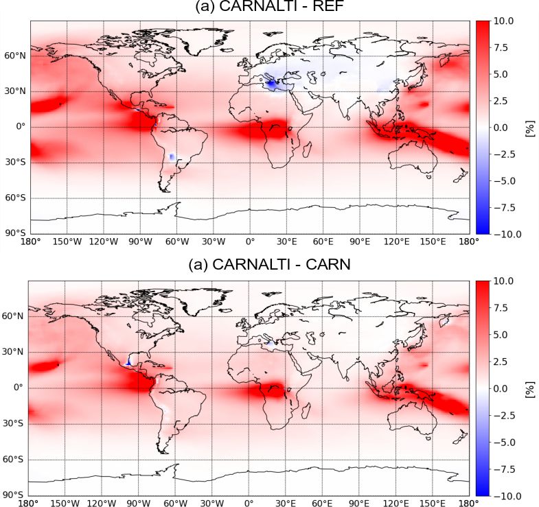
C. Lamotte et al.: Modeling study of the impact of volcanic emissions on the tropospheric sulfur budget                      11383

   Measurements were only carried out on sub-aerial vol-            instruments: TOMS, OMI and OMPS (Ozone Mapping and
canoes, i.e., emitting gases directly into the atmosphere. A        Profiler Suite) in the ultraviolet (UV), TIROS Operational
total of 69 volcanoes are listed in the inventory, divided          Vertical Sounder (TOVS), Atmospheric InfraRed Sounder
into two categories, namely 49 continuously erupting volca-         (AIRS) and Infrared Atmospheric Sounding Interferometer
noes and 25 sporadically erupting volcanoes. The following          (IASI) in the infrared (IR) and the Microwave Limb Sounder
five volcanoes belong to both categories because they had           (MLS) in the microwave range. Data from 119 volcanoes
a main activity of continuous emissions and also sporadic           and a total of 1502 events over the period are provided. For
eruptive events: Mount Aso, Augustine, Kı̄lauea East Rift           each of these eruptions, the information given includes the
Zone, Mayon and San Cristóbal.                                      location of the volcano (latitude and longitude), the date, the
   Since the beginning of volcanic emission measurements            VEI (Volcanic Explosivity Index), the estimated SO2 mass
in the early 1970s, the global activity of continuous eruptions     released (in kilotons) and also the height of the volcano and
has shown relative stability. The fluxes provided in the inven-     the height of the plume (measured if possible; estimated if
tory correspond to a temporal average of all measurements           not). Within our study, the additional information from Carn
for each volcano. Only three volcanoes are not concerned            et al. (2016) on the injection height is used (see details here-
by this hypothesis, i.e., Mount Etna in Sicily and Kı̄lauea         after), taking into account the height of the volcano as the
and the Kı̄lauea Rift Zone in Hawaii, which are known as            base of the emissions and the height of the plume as the top
being among the largest emitters of SO2 . For those volca-          of the injection.
noes, fluxes provided by specific studies (Andres and Kasg-            Second, the passive degassing data set is the first doc-
noc, 1998, personal communication) supersede the averages.          umented volcanic sulfur dioxide emission inventory made
   Since sporadic eruption data in Andres and Kasgnoc               with global satellite measurements (Carn et al., 2017). It was
(1998) are not recent, it is not possible to take them              retrieved from the observations of the OMI instrument in the
into account for the recent year chosen for the MOCAGE              UV spectrum during a long-term mission between 2005 and
simulation. Therefore, only continuous eruptions are used           2015. The high sensitivity of the instrument was a techno-
in MOCAGE and a global time-averaged SO2 flux of                    logical breakthrough that made it possible to distinguish low
13 Tg yr−1 is reported.                                             SO2 sources; this means ∼ 30 kt yr−1 for persistent anthro-
   Since no configuration was developed in MOCAGE to in-            pogenic sources and lower amounts (∼ 6 kt yr−1 ) for volca-
ject volcanic emissions aloft until this study, they were im-       noes which are located at higher altitudes or at lower latitudes
plemented in a similar manner to the other pollution sources.       that benefit from more satellite observations and optimal con-
Volcanic SO2 were thus emitted at the model surface (see            ditions (low solar zenith angle). The volcanic SO2 sources
Sect. 2.3). However, the surface elevation of the model (orog-      have been identified on the basis of 3-year averages (2005–
raphy) is mainly below the actual elevation of the volcanoes.       2007, 2008–2010 and 2011–2014), which implies that, for
                                                                    a source to be characterized as persistently degassing, the
3.2   New volcanic sulfur inventory                                 emission must be relatively constant on this timescale. An-
                                                                    nual mean emissions were calculated for each of the 90 vol-
With the improvements in satellite technology, an increasing        canic sources identified over the 11 years of the study. We as-
number of satellites are now able to better detect the sources      sume in the model that emission fluxes are constant through-
of volcanic SO2 , i.e., plume heights, quantities emitted and       out the year.
location. The most recent instruments with respect to TOMS,            Several parameters can affect the retrieval of volcanic
such as the Ozone Monitoring Instrument (OMI) and the               emissions, namely the measurement process, the calculation
TROPOspheric Monitoring Instrument (TROPOMI; Theys                  algorithm or the characterization of the type of emission.
et al., 2019), have a higher sensitivity to detecting small erup-   Thus, annual uncertainties are given with the mean annual
tions but also passive degassing. Global coverage gives an-         emissions for each volcano and each year. The total uncer-
other considerable advantage over other measurement tech-           tainty of the annual sulfur dioxide fluxes are estimated at
niques. As a reminder, COSPEC carries out measurements              55 % and over 67 % for sources emitting more than 100 and
from the ground and cannot be deployed on hard-to-access            less than 50 kt yr−1 , respectively. This latter information is
volcanoes.                                                          exploited in the sensitivity analysis (see Sect. 8). Note also
   The work of Carn et al. (2016, 2017) updates and adds            that, depending on the instrument used, the retrieval of the
complementary information to the study of Andres and Kas-           plume altitude can differ. Therefore, there are uncertainties
gnoc (1998) with a new inventory. The inventory is divided          on the altitude information provided by the inventory.
into two parts corresponding to the two types of emissions             Information on the altitude of volcanoes and on the plume
detectable by satellites.                                           height in the Carn et al. (2016) inventory is used to imple-
   First, the eruptive emissions data set (Carn et al., 2016,       ment a configuration to inject volcanic emissions aloft rather
with data available in Carn, 2021) is a synthesis of 40 years of    than keeping them at the model surface. This is an impor-
daily SO2 measurements (between 31 October 1978 and 31              tant improvement because, in some areas, depending on the
December 2018) derived from the following seven satellite           model resolution chosen, the model orography may differ

https://doi.org/10.5194/acp-21-11379-2021                                         Atmos. Chem. Phys., 21, 11379–11404, 2021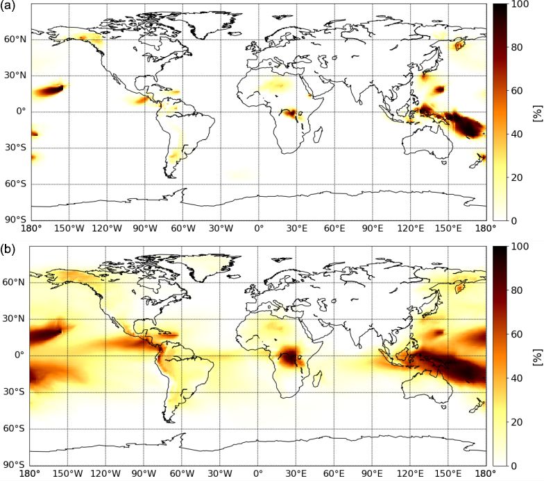
11384            C. Lamotte et al.: Modeling study of the impact of volcanic emissions on the tropospheric sulfur budget

from the actual topography and have an impact on the trans-
port of volcanic emissions. The new implementation sets the
passively degassing emissions at the model level of the vol-
cano altitude. For eruptions, the mass of SO2 emitted is dis-
tributed from the model level at the volcano vent to the model
level of the plume top height and follows an umbrella profile
similar to that used in other chemistry models (Freitas et al.,
2011; Stuefer et al., 2013). During a volcanic eruption, the
emitted materials (ashes and gases) are rapidly transported
vertically by the convection in the plume, and most of the
materials are concentrated at a high altitude, giving an um-
brella profile. In practice, the plume follows an almost linear
profile, with an increasing altitude from the volcano vent, and
then it opens into a parabola containing 75 % of the gases in
mass into the top third of the plume.
   In summary (see Table 1), the updated volcanic sulfur
emission inventory now includes about 160 volcanoes (∼
110 in the eruptive category and ∼ 90 in the passive de-
gassing category with 40 volcanoes in common). The avail-           Figure 1. Temporal evolution of 2013 SO2 emissions in Tg, the
ability of plume heights in this inventory allows a better rep-     non-volcanic emissions inventory for NOVOLC, plus the Andres
resentation of the injection of the volcanic emission in the        and Kasgnoc (1998) volcanic emissions inventory in REF or the
                                                                    Carn et al. (2016, 2017) volcanic emissions inventory in CARN and
model.
                                                                    CARNALTI.

4     Simulation setups and observations
                                                                    vious one. These two simulations are evaluated in Sect. 5,
4.1    Description of the simulations                               and the associated global distribution of sulfur species is
                                                                    compared in Sect. 6.
Meteorological fields are driven by the ARPEGE 3 hourly                In order to distinguish between the impact of the height of
forecasts. Anthropogenic and biomass burning sources                emission and of the quantity of SO2 emitted, another simu-
emit SO2 , whereas biogenic emissions from the ocean                lation, named CARN, is run and used for the analysis of the
are assumed to occur as DMS. Oceanic DMS emis-                      differences between the REF and CARNALTI global distri-
sions are 19.9 Tg S yr−1 , while anthropogenic emissions are        bution of sulfur species. Volcanic emissions are from Carn
48.6 Tg S yr−1 . For 2013, biomass burning emissions from           et al. (2016, 2017), as in CARNALTI, but they are injected at
GFAS products were relatively low, at only 1 Tg S yr−1 .            the model surface, as in REF.
   Concerning volcanic sulfur emission invento-                        CARNALTI is run to provide a better representation of the
ries, either Andres and Kasgnoc (1998) or Carn                      global tropospheric sulfur. This is why it is selected for the
et al. (2016, 2017) is used. The full eruption emis-                analysis of the tropospheric sulfur budget in Sect. 7. In or-
sion database is available following Carn (2021,                    der to quantify the contribution of the volcanoes in the sulfur
https://doi.org/10.5067/MEASURES/SO2/DATA405).                      budget, we compare CARNALTI to the NOVOLC simula-
   In total, four different simulations (Table 2) are carried out   tion that does not take into account volcanic emissions (only
in order to evaluate the impact induced by the update of the        anthropogenic, biomass burning and dust).
volcanic SO2 inventory in MOCAGE and to analyze its con-               The four simulations are run for the year 2013 with a
tribution to the sulfur species budget in the atmosphere at the     3 month spin-up period (from October to December 2012).
global scale. The four simulations are run at a resolution of       In addition to being one of the years for which a large amount
1◦ × 1◦ .                                                           of observational data is available globally, 2013 is chosen as
   The first simulation, named REF, takes into account the          the year with the lowest eruptive emission flux (Carn et al.,
previous volcanic inventory (from Andres and Kasgnoc,               2016). Figure 1 shows the volcanic emissions of the different
1998) with the injection at the model surface. The second           simulations for the year 2013. We notice the monthly varia-
simulation, named CARNALTI, uses the updated volcanic               tion due to non-volcanic emissions (NOVOLC run in green),
inventory (from Carn et al., 2016, 2017) and the new con-           with fewer emissions during the Northern Hemisphere sum-
figuration to inject volcanic emissions from the volcano al-        mer and the highest values in the Northern Hemisphere win-
titude, as described in Sect. 3.2. By comparing REF and             ter. Volcanic emissions from Andres and Kasgnoc (1998) are
CARNALTI runs, we can analyze the changes brought by the            steady throughout the year, as we can see in the REF run
updated volcanic emission inventory with respect to the pre-        (in blue). They are lower than the volcanic emissions of the

Atmos. Chem. Phys., 21, 11379–11404, 2021                                           https://doi.org/10.5194/acp-21-11379-2021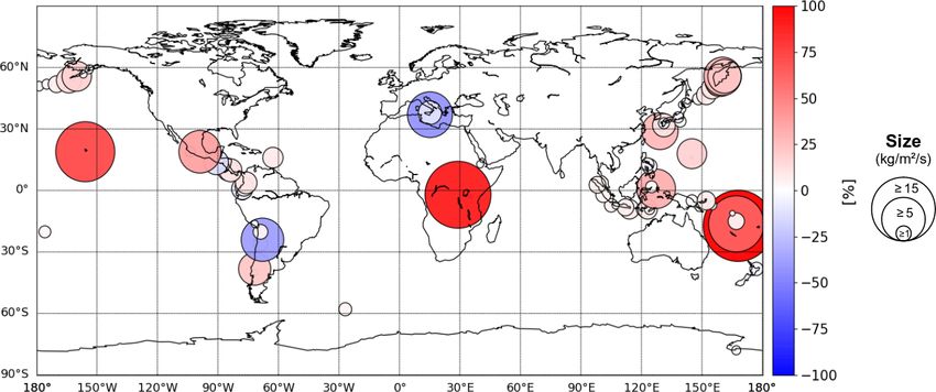
C. Lamotte et al.: Modeling study of the impact of volcanic emissions on the tropospheric sulfur budget                                  11385

Table 1. Summary of the main characteristics of the previous (Andres and Kasgnoc, 1998) and the updated (Carn et al., 2016, 2017) SO2
volcanic emission inventories.

                                  Previous volcanic inventory                                   New volcanic inventory
                                  Andres and Kasgnoc (1998)            Carn et al. (2016)                   Carn et al. (2017)
   Emission type                  Continuous emissions                 Eruption                             Passive degassing
   Period                         1970–1997                            1978–2018                            2005–2018
   Instruments                    COSPEC and TOMS                      Satellite instruments (seven)        OMI
   Frequency                      Time-averaged over the period        Daily total quantity per volcano     Annual mean quantity per volcano
   Information on the vertical    No information                       Volcano altitude                     Volcano altitude and plume height
   No. of volcanoes               43                                   119                                  91

Table 2. Main features of the simulations.

                                                 Volcanic inventory                 Altitude of injection
                             REF                 Andres and Kasgnoc (1998)          At model surface
                             CARNALTI            Carn et al. (2016) – eruption      From volcano vent to plume top
                                                 Carn et al. (2017) – degassing     At volcano vent
                             CARN                Carn et al. (2016, 2017)           At model surface
                             NOVOLC              n/a                                n/a

                           Note: n/a: not applicable.

CARNALTI and CARN runs (in red), with strong constant                       (GOME-2) Metop-A (Meteorological Operational satellite)
passive degassing throughout the year and a few sporadi-                    instrument being at the end of its lifetime, data retrievals
cally eruptive events. Indeed, Andres and Kasgnoc (1998)                    are not good enough and present strong artifacts, as is the
SO2 emissions are 13 Tg (or 6.5 Tg S), while the total 2013                 case for GOME-2 Metop-B. Therefore, we choose the OMI,
annual emissions in Carn et al. (2016, 2017) are 23.7 Tg of                 which is the most widely used (e.g., He et al., 2012; Fiole-
SO2 (or 11.8 Tg S), with 23.5 Tg of passive degassing SO2                   tov et al., 2013; Wang et al., 2017; Wang and Wang, 2020).
and 0.2 Tg of eruptive emissions (< 1 % of the total amount                 Moreover, the SO2 tropospheric column estimated from the
of volcanic SO2 emissions, which is almost negligible).                     OMI is the finest resolution and most accurate instrument
   Figure 2 spatially represents the difference between the                 from 2013 for retrieving SO2 total columns over passively
previous and the new inventories. The red dots mostly show                  emitted volcanoes with altitudes that are generally around
new volcanoes in Carn et al. (2016, 2017) which are not ac-                 2–3 km. For aerosols, there is no satellite-derived product
counted for by Andres and Kasgnoc (1998). However, we                       providing information on sulfate only. Nevertheless, satellite
also notice blue dots, meaning that, in the new inventory, the              observations of aerosols as a whole are available. Here, we
estimated emission fluxes are reduced. Given the low number                 choose MODIS (Moderate-Resolution Imaging Spectrora-
of eruptive emissions in 2013, the annual average of volcanic               diometer) aerosol optical depth (AOD), which provides data
emissions in Fig. 2 essentially represents passive emissions.               at the global scale. MODIS AOD is known as being a robust
                                                                            product and is used in the literature for global evaluation and
4.2   Observations used for the evaluation of the                           aerosols assimilation in models (e.g., Liu et al., 2011; Dai
      simulations                                                           et al., 2014; Sič et al., 2015; Guth et al., 2016, 2018). The
                                                                            model comparison with MODIS AOD provides an indirect
                                                                            evaluation for sulfate aerosols since AOD includes sulfate
We use satellite-based instruments for the model evaluation
                                                                            aerosols.
since they provide a global sampling. The target chemical
species that we evaluate are SO2 and aerosols, since SO2 is
the precursor of sulfate aerosols. Concerning SO2 , observa-                4.2.1     OMI SO2 total column
tions in the infrared are not suitable since passive degassing
occurs mostly under 5 km, at altitudes where such instru-                   The Aura Ozone Monitoring Instrument (OMI) level 2 sul-
ments have reduced sensitivity (Carboni et al., 2012; Taylor                fur dioxide (SO2 ) total column product (Li et al., 2020)
et al., 2018). Therefore, observations in UV-visible range are              was used to validate the model simulations. This product
chosen. With the Global Ozone Monitoring Experiment–2                       has been available since 2004. The resolution of the data

https://doi.org/10.5194/acp-21-11379-2021                                                     Atmos. Chem. Phys., 21, 11379–11404, 2021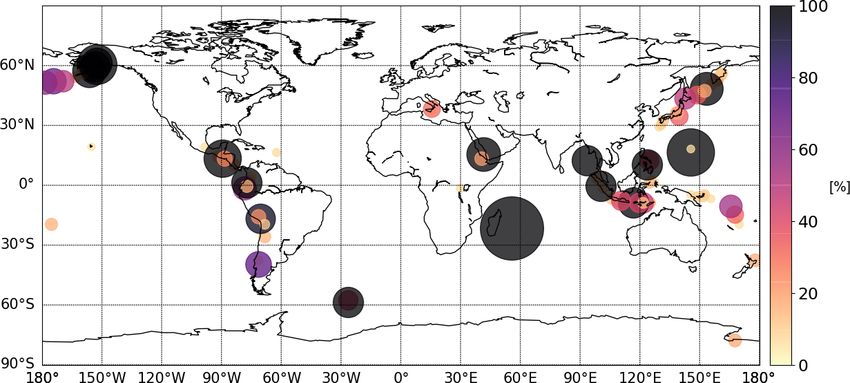
11386            C. Lamotte et al.: Modeling study of the impact of volcanic emissions on the tropospheric sulfur budget

Figure 2. The 2013 annual average ratio between volcanic SO2 emissions in the Carn et al. (2016, 2017) and Andres and Kasgnoc (1998)
inventories. The size of the circles represents the absolute difference in kilograms per meter per second (kg m−2 s−1 ), while the color
represents the relative difference in percent.

is 13 km × 24 km at the nadir. The retrieval algorithm is             4.2.2    MODIS aerosol optical depth
a principal component analysis (PCA)-based algorithm (Li
et al., 2013). Various physical and technical causes can re-          We use daily level 3 MODIS data (MOD08, Terra; MYD08,
duce the quality of data. Thus, pre-processing and data fil-          Aqua; collection 6.1) for the year 2013. Before use, we per-
tering were applied as recommended to select only the best            formed additional quality control and screening (Sič et al.,
possible observations. Pixels with large solar zenith angles          2015; Guth et al., 2016). These treatments aim at minimiz-
(SZAs > 65◦ ), affected by the South Atlantic Anomaly re-             ing cloud contamination and avoid low-confidence measure-
gion (Richter et al., 2006), on the edge of the swaths or the         ments (Zhang et al., 2005; Koren et al., 2007; Remer et al.,
OMI row anomaly (signal suppression at certain OMI rows;              2008). Moreover, all AOD values below 0.05 are automati-
see Schenkeveld et al., 2017) and pixels with a cloud frac-           cally filtered out because Ruiz-Arias et al. (2013) highlighted
tion greater than 30 % or flagged with low-confidence data            the rapid growth in the relative underestimation of AODs af-
are removed.                                                          ter this threshold, which leads to a mean relative error above
   There are various products available in the OMI data set           50 %.
since the OMI instrument has a variable sensitivity, depend-             In MOCAGE, AODs are calculated using Mie theory with
ing on altitude, and the retrieval of SO2 requires the use            the Global Aerosol Data Set’s refractive indices (Köpke
of an a priori profile. The first product selected, named             et al., 1997) and extinction efficiencies derived with the Mie
Column_Amount_SO2 , is an estimate of SO2 vertical col-               scattering code for homogeneous spherical particles from
umn density (VCD) and constrained by the GEOS-5 global                Wiscombe (1980).
model a priori profiles. Then, three specific products with
adapted a priori profiles are also available and selected. One,       4.3     Statistical metrics used for evaluation
named Column_Amount_SO2 _PBL, is an estimate of the
SO2 vertical column density (VCD), with an a priori pro-              In order to evaluate the model against observation data, we
file assuming that the essence of SO2 is in the boundary layer        use the fractional bias, the fractional gross error, the root
(within the lowest 1 km of the atmosphere). Another product,          mean square error and the correlation coefficient, following
named Column_Amount_SO2 _TRL, is almost the same as                   Seigneur et al. (2000).
the previous one but assumes a lower tropospheric SO2 pro-               The fractional bias or modified normalized mean bias
file (with a center of mass altitude at 3 km). The last product       (MNMB) quantifies the mean between the modeled (f ) and
selected, named Column_Amount_SO2 _TRM, corresponds                   the observed (o) elements, for N observations. It ranges be-
to an assumed middle tropospheric SO2 profile (with a cen-            tween −2 and 2 and varies symmetrically with respect to
ter of mass altitude at 8 km).                                        the under- and overestimation of the model. The definition
                                                                      is given by the following:

                                                                                      N
                                                                                   2 X   fi − o i
                                                                      MNMB =                      .                                 (1)
                                                                                   N i=1 fi + oi

Atmos. Chem. Phys., 21, 11379–11404, 2021                                              https://doi.org/10.5194/acp-21-11379-2021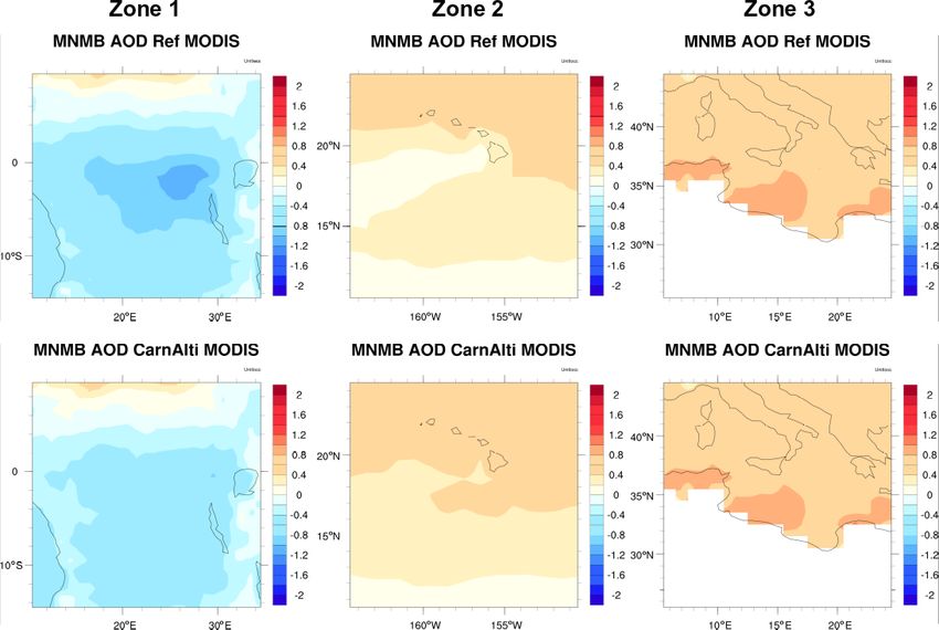
C. Lamotte et al.: Modeling study of the impact of volcanic emissions on the tropospheric sulfur budget                       11387

   The fractional gross error (FGE) quantifies the model er-        each daily OMI SO2 total column measurements, and then
ror. It is a positive variable ranging between 0 and 2. The         we perform an annual average for each of the 633 data points.
definition is given by the following:                               Similar to the abovementioned studies, the results are shown
                                                                    as scatterplots, and the statistical metrics used are the corre-
             N
          2 X   fi − oi                                             lation coefficient and the RMSE.
FGE =                   .                                    (2)
          N i=1 fi + oi                                                In total, two methods are used in the evaluation strategy.
                                                                    First, we choose to evaluate the model SO2 total column
   The root mean square error (RMSE) is the square root of          against OMI Column_Amount_SO2 product. However, in or-
the average of the squared difference between each model            der to test if the evaluation is sensitive to this choice, we use
and observation value. In other words, it represents a mea-         another approach which consists of an interpolation of OMI
sure of the accuracy in absolute values, while FGE is relative.     SO2 observations at the altitude where the volcanic emissions
RMSE is a positive variable, and a value of 0 (almost never         are injected in MOCAGE. To do so, we use the OMI products
achieved in practice) would indicate a perfect fit to the data.     Column_Amount_SO2 _PBL, Column_Amount_SO2 _TRL
The formula is given by the following:                              and Column_Amount_SO2 _TRM, hereafter renamed PBL,
           v                                                        TRL and TRM, respectively. Depending on the altitude of
           u
           u1 X  N                                                  the emissions in MOCAGE, either PBL and TRL or TRL
RMSE = t            (fi − oi )2 .                           (3)     and TRM are used for the interpolation.
              N i=1                                                    Concerning the AODs, a spatial validation on the whole
                                                                    global domain is possible against MODIS products. The
   The correlation coefficient (R) indicates whether the vari-      evaluation at the global scale enables us to quantify the over-
ations in the model and the observations are well matched           all aerosol changes in the simulations from the use of the
and ranges between −1 and 1. The closer the score is to 0,          updated inventory with respect to the previous one. Since
the weaker the correlation is. The definition is given by the       noticeable changes are also expected at the local scale in
following:                                                          the vicinity of the volcanoes, three zones are selected to
       1 PN                                                         complete the global-scale evaluation against MODIS. These
       N  i=1 (fi− f )(oi − o)                                      zones are chosen from among the largest passive SO2 emit-
R=                             ,                             (4)
                σf σo                                               ters in Carn et al. (2017) and are representative of different
                                                                    types of changes between Andres and Kasgnoc (1998) and
where f and o are, respectively, the model and observations         Carn et al. (2016, 2017) volcanic emissions inventories.
mean values, and σf and σo are the standard deviations from            Zone 1 is centered over central Africa and is under the
the modeled and observed time series.                               influence of Mount Nyiragongo and Nyamuragira (altitude of
                                                                    2950 m). In Andres and Kasgnoc (1998), this volcano is not
5     Evaluation of the simulations                                 listed. In contrast, in Carn et al. (2017), the passive degassing
                                                                    emission represents 2.29 Tg in 2013. No eruption is listed in
5.1    Evaluation strategy                                          Carn et al. (2016) for 2013.
                                                                       Zone 2 is located in the northern Pacific Ocean around
For the evaluation of the simulations, OMI and the MODIS            Hawaii. The volcano, based on the island, is Kı̄lauea (alti-
data set are mapped at the model resolution (1◦ × 1◦ ). The         tude of 1222 m). In the REF simulation, the volcano emis-
model grid points in the simulations corresponding to the           sions in the inventory are 0.45 Tg yr−1 (seventh rank of the
filtered observation pixels (as explained in Sect. 4.2.1 and        most SO2 -emitting volcanoes in Andres and Kasgnoc, 1998).
4.2.2) are also removed. A different validation strategy is ap-     But, in Carn et al. (2017), the Kı̄lauea emissions are updated,
plied, depending on the instrument.                                 and it is the second-biggest emitter, with 2.17 Tg. In 2013, no
    Concerning OMI SO2 total columns, similarly to other            eruptions are recorded in Carn et al. (2016) for this area.
SO2 satellite-derived products, their relative uncertainties are       Zone 3 is located in the Mediterranean region, under the
large where the signal is low, in particular for background         influence of Mount Etna (altitude of 2711 m in the inventory)
conditions. This is why, in the literature, the SO2 satellite       and Stromboli (altitude of 870 m in the inventory). In Andres
comparisons and the model evaluations focus on specific ar-         and Kasgnoc (1998), 1.48 Tg yr−1 is emitted by Mount Etna
eas close to SO2 sources (e.g., He et al., 2012; Fioletov et al.,   (the biggest volcanic SO2 -emitter referenced), 0.27 Tg yr−1
2013; Wang and Wang, 2020). Similar to these studies, our           is emitted by Stromboli and also 0.02 Tg yr−1 by Vulcano.
strategy is to perform the model evaluation only in the vicin-      In Carn et al. (2016, 2017), only 0.65 Tg of SO2 are emit-
ity of the volcanic sources. For each volcano, based on those       ted in 2013 in zone 3, corresponding to less than 0.04 Tg for
referenced in Carn et al. (2016, 2017), we select nine model        Stromboli and 0.61 Tg for Mount Etna. Vulcano is not in the
grid points (representing a square of 3◦ ×3◦ ), with the middle     Carn et al. (2016, 2017) inventories. In 2013, small eruptions
point being where the volcano is located (see Fig. 3). Alto-        occurred at Mount Etna, totaling a little less than 0.06 Tg.
gether, it corresponds to 633 points. The mask is applied on        Therefore, in the updated Carn et al. (2016, 2017), volcanic

https://doi.org/10.5194/acp-21-11379-2021                                         Atmos. Chem. Phys., 21, 11379–11404, 2021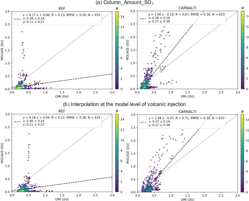
11388 C. Lamotte et al.: Modeling study of the impact of volcanic emissions on the tropospheric sulfur budget
Figure 3. Location of the selected areas where OMI SO2 total column are selected for the validation. They correspond to nine MOCAGE
grid points around each volcano from Carn et al. (2016, 2017).
emissions in zone 3 are weaker than in Andres and Kasgnoc and in the OMI retrieval products used for the model evalua-
(1998). tion.
For the evaluation of the simulations against MODIS, the
statistical metrics used are the MNMB, FGE and correla- Validation against MODIS AOD at 550 nm
tion coefficient. Because MNMB and FGE are dimension-
less, they are meaningful in all geographical regions regard- As a second evaluation step, we compare the simulations’
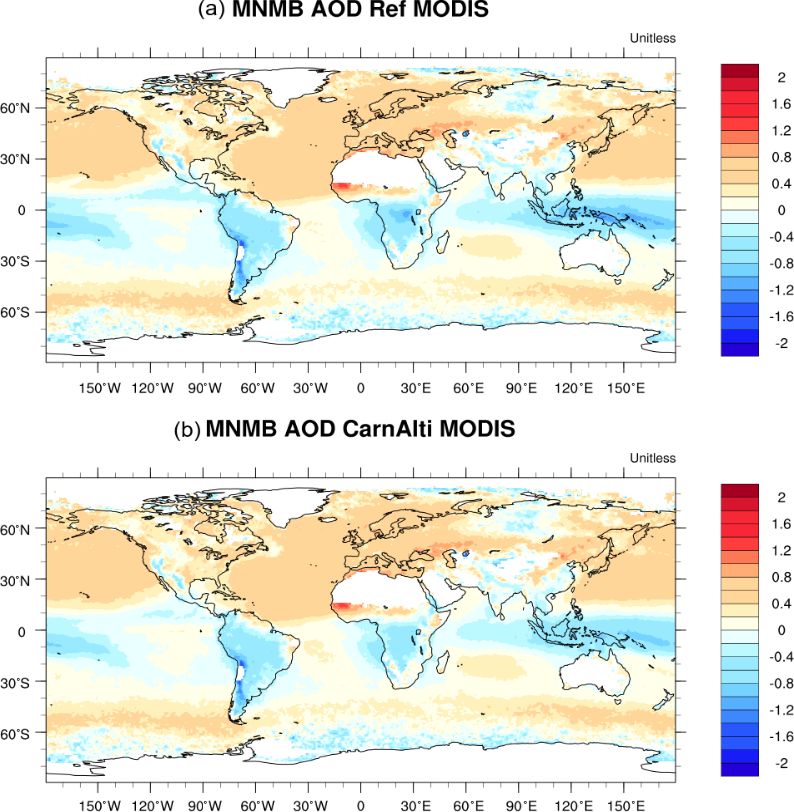
less of the magnitude of the aerosol column. AOD with the AOD from MODIS. Figure 5 presents, for the
REF and CARNALTI experiments, the 2013 annual MNMB
5.2 Validation against OMI SO2 total column with respect to MODIS AOD observations. We can see that
the equatorial belt has a negative MNMB, between −0.2 and
Figure 4a presents the scatterplots of MOCAGE SO2 −1.2 in the REF simulation, but in the CARNALTI sim-
columns in DUs (Dobson units) from the REF and ulation, it is closer to 0; e.g., in the vicinity of volcanoes
CARNALTI simulations against OMI observations based on in Indonesia or in central Africa. This shows an improve-
GOES-5 a priori profiles. Each of the points represents an av- ment in the MOCAGE AOD modeling at the global scale by
erage over the 2013 year. It shows that the previous version of updating the volcanic emissions inventory. Despite the im-
the model (REF) was not good. The correlation coefficient is provement in MNMB in the areas near volcanoes, the over-
low (0.13). The bias is high, with a mean SO2 measured by all score is not improved (see Table 3). Indeed, the MNMB
OMI of 0.28 DU and of 0.11 in REF simulation. With the of the Northern Hemisphere is mainly positive and almost
new volcanic inventory in the CARNALTI simulation, the unchanged with the new inventory (Carn et al., 2016, 2017)
mean SO2 concentration is similar to OMI retrievals (0.27). in which only a few volcanoes are reported. Even this small
We can also clearly see an improvement of the model perfor- number of volcanoes, locally, leads to an increase in the al-
mances with a correlation increased up to 0.67. ready positive MNMB. Thus, globally, the average MNMB
To evaluate the impact of the choice of OMI product, we is higher in CARNALTI than in REF.
also show in Fig. 4 (bottom row) the scatterplot when apply- Concerning the fractional gross error (FGE), changes are
ing the interpolation at the MOCAGE altitude where volcanic also located in the vicinity of volcanoes (see Fig. S1 in the
emissions are injected. This method provides higher OMI Supplement). In those areas, especially in central Africa and
estimates and, therefore, increases the bias with MOCAGE in Indonesia, the FGE is reduced from a maximum of 1.2
simulations, but it improves the correlation. The conclusion in REF to a maximum of 0.6 in CARNALTI. Globally, the
is that the CARNALTI simulation provides by far better sta- FGE score is slightly improved, with 0.43 for REF and 0.42
tistical results (bias, RMSE and correlation) than REF. The in CARNALTI. Even if, locally in the Northern Hemisphere
negative bias of MOCAGE CARNALTI with respect to OMI (e.g., in Hawaii), the FGE score can be deteriorated in the
could be due to errors in the plume transport in the model simulation with Carn et al. (2016, 2017), at the global scale,
linked to uncertainties in the meteorological inputs, to the the new inventory is better.
limited number of model vertical levels, to the model chem- The correlation coefficient R score is better in the North-
istry and/or aerosol scheme or also to the uncertainties in the ern Hemisphere (see Fig. S1). Therefore, by adding new vol-
SO2 emission estimates from OMI in Carn et al. (2016, 2017) cano point sources, and mostly in the Southern Hemisphere,
Atmos. Chem. Phys., 21, 11379–11404, 2021 https://doi.org/10.5194/acp-21-11379-2021C. Lamotte et al.: Modeling study of the impact of volcanic emissions on the tropospheric sulfur budget 11389
Figure 4. Scatterplots of annual mean OMI SO2 versus MOCAGE simulations (left – REF; right – CARNALTI) (a) considering total columns
and (b) interpolating at the model level where volcanic emissions are injected. Also shown are the 1 : 1 line (solid gray), linear regression
line (black dash), linear regression formula, correlation coefficient (R), root mean squared error (RMSE), number of collocated pairs (N),
OMI mean and standard deviation in DU (x), MOCAGE mean and standard deviation in DU (y) and density of collocated pairs (color bar).
Table 3. The 2013 annual statistics of the REF and CARNALTI simulations against MODIS observations on specific zones.
Globe Zone 1 Zone 2 Zone 3
MNMB FGE R MNMB FGE R MNMB FGE R MNMB FGE R
REF 0.10 0.43 0.35 −0.47 0.56 0.75 0.31 0.35 0.74 0.704 0.715 0.632
CARNALTI 0.12 0.42 0.35 −0.34 0.44 0.74 0.39 0.41 0.78 0.699 0.711 0.632
the scores are higher in CARNALTI. The lifetime of aerosols of the Nyamuragira volcanic SO2 emissions. The MNMB is
increases when located in a higher altitude. Aerosols are bet- largely reduced in CARNALTI simulation.
ter represented in the CARNALTI simulation thanks to the In zone 2, unlike the previous area, the MNMB is already
use of a better injection altitude of SO2 (a precursor of sul- positive. Thus, by adding more SO2 volcanic emissions, it
fate aerosols contributing to the AOD). increases the sulfate aerosol content, leading to a deteriora-
By using Carn et al. (2017), the model results are improved tion of the MNMB and FGE scores (Table 3). The corre-
in zone 1. The MNMB rises from −0.47 with the REF sim- lation coefficient increases due to a more accurate altitude
ulation to −0.34 in the CARNALTI run. Similarly, the FGE where the emissions are injected in the CARNALTI simula-
is improved. In Fig. 6 (left column for zone 1), the nega- tion. Figure 6 in the middle column confirms these results.
tive MNMB score in the REF simulation highlights the lack However, with the volcano being located at an altitude of
1222 m, where the sensitivity of, mostly, infrared but also
https://doi.org/10.5194/acp-21-11379-2021 Atmos. Chem. Phys., 21, 11379–11404, 202111390 C. Lamotte et al.: Modeling study of the impact of volcanic emissions on the tropospheric sulfur budget
6 Impact of the volcanic emission inventory update on
the species concentration
SO2 , sulfate aerosols and PM2.5 tropospheric column and
surface concentrations are summarized in Table 4. In order to
dissociate the effect of the quantity of SO2 emitted and of the
injection altitude, we compare the REF and CARNALTI sim-
ulations with the CARN run. The annual mean sulfur diox-
ide total column, at the global scale, is 1.68 × 10⁻⁵ mol m−2
in the CARNALTI simulation, which is 13 % higher than
the 1.49×10⁻⁵ mol m−2 in REF. Regarding aerosols species,
sulfate total column is 23 % higher in the CARNALTI sim-
ulation, but only by 1 % for PM2.5 , because it is only par-
tially composed of sulfate. This increase is explained by the
greater amount of SO2 emitted in Carn et al. (2016, 2017)
and by the new injection configuration. At higher altitudes,
the lifetime of sulfur species is longer due to slower removal
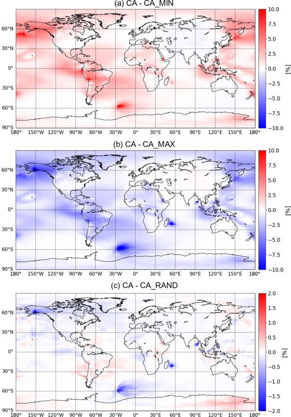
processes (Stevenson et al., 2003). Figure 7 illustrates this
concept. It shows the relative difference in the sulfate tro-
pospheric column between the CARNALTI and REF experi-
ments. We clearly see an increase in CARNALTI concentra-
tions in the vicinity of most volcanic point sources.
Figure 5. Maps of the 2013 annual MNMB of aerosol opti-
Surface concentrations, at the global scale, from the sim-
cal depth against MODIS monthly observations for (a) REF and
ulations show different results. With 3.71 × 10⁻¹⁰ kg m−3
(b) CARNALTI simulations.
in the REF simulation, sulfate is lower than in the
CARNALTI simulation, with 3.99 × 10⁻¹⁰ kg m−3 (+8 %).
However, concerning SO2 surface concentrations, with
ultraviolet instruments is reduced, the estimation in the in- 1.08 × 10⁻⁸ mol m−3 , there is more SO2 in the REF than in
ventory for this volcano may be overestimated. the CARNALTI simulation, with only 1.02 × 10⁻⁸ mol m−3 .
In zone 3, the statistical scores are almost similar for the Even if there are more volcanic SO2 emissions in the
two simulations. Indeed, in this region there are various other CARNALTI run, by injecting it in altitude, sulfur dioxide
aerosols sources (industries, transport, dust, etc.), and sul- remains in the atmosphere longer and reaches the surface
fate from volcanic emissions does not dominate. Still, we can less. But, in the CARN simulation results, where the volcanic
see, in Fig. 6, a small improvement in MNMB between the emissions are injected at the model surface, we notice higher
REF and CARNALTI simulations. The FGE and correlation concentrations of SO2 at the surface (1.14 × 10⁻⁸ mol m−3 ).
scores are also a bit better in CARNALTI. Thus, using Carn The mean sulfate aerosol concentrations in the CARN simu-
et al. (2016, 2017) and injecting volcanic emissions at the lation are 3.85 × 10⁻¹⁰ kg m−3 . This is 4 % higher than in
actual altitude of the volcanoes slightly enhances MOCAGE the REF simulation (as seen before) but also almost 4 %
performances. lower than in the CARNALTI simulation. Indeed, compared
to REF, with more volcanic emissions, there is more forma-
tion of sulfate (such as in the CARNALTI run). However, due
5.3 Summary of the evaluation to being emitted at the surface, sulfate aerosols are rapidly
removed by deposition in CARN compared to CARNALTI.
The evaluation of MOCAGE performances against the OMI Figure 7 shows this difference in the transport of sulfate
SO2 total column and MODIS AOD shows an improvement aerosols. In the CARNALTI simulation, we can clearly see
in the CARNALTI simulation compared to REF. The previ- the volcanic plumes spreading further from the volcanoes,
ous inventory (Andres and Kasgnoc, 1998) lacks some vol- almost 150 to 200 km away.
canic sources, which leads to a global underestimation of sul- By looking at the local scale, the differences between
fur dioxide concentrations and aerosol concentrations in the CARNALTI and REF can be very large. For example, in
tropics (e.g., in zone 1). With the new inventory (Carn et al., zone 1, the SO2 tropospheric column is 3 times larger in
2016, 2017) used in the CARNALTI simulation, volcanic CARNALTI (from 1.07 × 10⁻⁵ mol m−2 in REF to 3.31 ×
emissions are larger. Even if in some areas the scores are de- 10−5 mol m−2 ), 2 times larger for the aerosol sulfate total
teriorated, e.g., in zone 2 where the model is already overes- column (from 3.80 × 10⁻⁶ to 8.30 × 10⁻⁶ kg m−2 ) and al-
timating aerosol concentrations, the scores at the global scale most twice as large for sulfate at the surface (4.59 × 10⁻¹⁰
and in the vicinity of most of the volcanoes are improved. to 7.95 × 10⁻¹⁰ kg m−3 ). In zone 2, changes are also more
Atmos. Chem. Phys., 21, 11379–11404, 2021 https://doi.org/10.5194/acp-21-11379-2021You can also read