CM2MC-LPJML V1.0: BIOPHYSICAL COUPLING OF A PROCESS-BASED DYNAMIC VEGETATION MODEL WITH MANAGED LAND TO A GENERAL CIRCULATION MODEL - GMD
←
→
Page content transcription
If your browser does not render page correctly, please read the page content below

Geosci. Model Dev., 14, 4117–4141, 2021
https://doi.org/10.5194/gmd-14-4117-2021
© Author(s) 2021. This work is distributed under
the Creative Commons Attribution 4.0 License.

CM2Mc-LPJmL v1.0: biophysical coupling of a process-based
dynamic vegetation model with managed land to a general
circulation model
Markus Drüke1,2 , Werner von Bloh1 , Stefan Petri1 , Boris Sakschewski1 , Sibyll Schaphoff1 , Matthias Forkel3 ,
Willem Huiskamp1 , Georg Feulner1 , and Kirsten Thonicke1
1 Potsdam   Institute for Climate Impact Research, Member of the Leibniz Association, 14412 Potsdam, Germany
2 Humboldt    University of Berlin, Department of Physics, 12489 Berlin, Germany
3 Institute of Photogrammetry and Remote Sensing, Dresden University of Technology, 01069 Dresden, Germany

Correspondence: Markus Drüke (drueke@pik-potsdam.de)

Received: 23 December 2020 – Discussion started: 18 February 2021
Revised: 19 May 2021 – Accepted: 30 May 2021 – Published: 1 July 2021

Abstract. The terrestrial biosphere is exposed to land-use      performance of LPJmL5 in the coupled system compared to
and climate change, which not only affects vegetation dy-       Earth observation data and to LPJmL offline simulation re-
namics but also changes land–atmosphere feedbacks. Specif-      sults is within acceptable error margins. The historical global
ically, changes in land cover affect biophysical feedbacks of   mean temperature evolution of our model setup is within the
water and energy, thereby contributing to climate change. In    range of CMIP5 (Coupled Model Intercomparison Project
this study, we couple the well-established and comprehen-       Phase 5) models. The comparison of model runs with and
sively validated dynamic global vegetation model LPJmL5         without land-use change shows a partially warmer and drier
(Lund–Potsdam–Jena managed Land) to the coupled climate         climate state across the global land surface. CM2Mc-LPJmL
model CM2Mc, the latter of which is based on the atmo-          opens new opportunities to investigate important biophysi-
sphere model AM2 and the ocean model MOM5 (Modular              cal vegetation–climate feedbacks with a state-of-the-art and
Ocean Model 5), and name it CM2Mc-LPJmL. In CM2Mc,              process-based dynamic vegetation model.
we replace the simple land-surface model LaD (Land Dy-
namics; where vegetation is static and prescribed) with
LPJmL5, and we fully couple the water and energy cycles
using the Geophysical Fluid Dynamics Laboratory (GFDL)          1   Introduction
Flexible Modeling System (FMS). Several improvements to
LPJmL5 were implemented to allow a fully functional bio-        Human activities, including land-use change and fossil fuel
physical coupling. These include a sub-daily cycle for calcu-   emissions, alter the climate and lead to profound changes in
lating energy and water fluxes, conductance of the soil evap-   the components of the Earth system and their interactions.
oration and plant interception, canopy-layer humidity, and      For example, increasing managed land for agriculture and
the surface energy balance in order to calculate the surface    other human activities not only reduces natural vegetation
and canopy-layer temperature within LPJmL5. Exchanging          cover but also changes how energy, water and carbon are
LaD with LPJmL5 and, therefore, switching from a static and     exchanged between land, atmosphere and ocean. However,
prescribed vegetation to a dynamic vegetation allows us to      a functioning biosphere ensures stable energy, carbon and
model important biospheric processes, including fire, mor-      water cycles; hence, the atmospheric composition and radia-
tality, permafrost, hydrological cycling and the impacts of     tive forcing are maintained. While plants sequester carbon
managed land (crop growth and irrigation). Our results show     dioxide (CO2 ), they also contribute to water cycling, albedo
that CM2Mc-LPJmL has similar temperature and precipi-           and roughness length, influencing the exchange of energy on
tation biases to the original CM2Mc model with LaD. The         multiple timescales (Green et al., 2017; Chapin et al., 2008;

Published by Copernicus Publications on behalf of the European Geosciences Union.
4118                                                                                        M. Drüke et al.: CM2Mc-LPJmL

Heyder et al., 2011). These effects can alter the regional and     amplified by factors such as increased tree mortality, which
global climate and, in turn, lead to changes in land vege-         then changes land-surface characteristics over time (Quillet
tation. To address the implications of climate and land-use        et al., 2010). Hence, a bidirectional and stable coupling of a
change on vegetation dynamics and land–atmospheric feed-           DGVM with a full water, energy and carbon cycle remains
backs, Earth system models (ESMs) with embedded dynamic            challenging (Forrest et al., 2020; Pokhrel et al., 2016).
vegetation components are required.                                   In this study, we introduce the biophysical coupling of
   ESMs increasingly incorporate dynamic global vegetation         water and energy fluxes resulting from vegetation dynam-
models (DGVMs) to advance from quantifying only simple             ics as simulated by the adapted whole-ecosystem Lund–
fluxes of carbon, energy and water from land to also cap-          Potsdam–Jena managed Land (LPJmL5) DGVM (Schaphoff
turing climate feedbacks that result from changes in vegeta-       et al., 2018b; Von Bloh et al., 2018) with the Geophys-
tion cover due to plant mortality and regrowth (Quillet et al.,    ical Fluid Dynamics Laboratory (GFDL) coupled model
2010; Forrest et al., 2020; Viterbo, 2002; Pokhrel et al., 2016;   CM2 (Milly and Shmakin, 2002) in a coarse-resolution
Fisher et al., 2018; Mueller and Seneviratne, 2014; Hajima         setup called CM2Mc (Galbraith et al., 2011). The flexi-
et al., 2020; Green et al., 2017). Originally, DGVMs were          ble modeling system (FMS; Balaji, 2002) is used to couple
developed as stand-alone vegetation models to quantify cli-        the terrestrial biosphere, modeled by LPJmL5, to the other
mate change impacts on terrestrial vegetation (Prentice et al.,    ESM model components. In this new model configuration,
2007). However, over the last 2 decades, they have evolved         CM2Mc-LPJmL v1.0, LPJmL5 supplies the variables neces-
into whole-ecosystem models, capturing a wide range of             sary for the coupling (canopy temperature, canopy humidity,
biospheric processes for natural and managed vegetation,           albedo and roughness length), thereby replacing the original
and simulating global carbon, energy and water fluxes with         LaD GFDL land-surface model (Milly and Shmakin, 2002)
a good modeling skill when compared to observation data            in the CM2Mc setup. To accomplish the interactive coupling
(e.g., Schaphoff et al., 2018a). Therefore, embedding these        between LPJmL5 and CM2Mc, additional quantities which
whole-ecosystem DGVMs in ESMs allows one to quantify               were not part of the stand-alone LPJmL5 (e.g., the tempera-
which ecosystem response or change in land use can cause           ture and canopy humidity) were introduced. The benefits of
climate feedbacks and could have wider implications for the        coupling LPJmL5 include the use of the process-based SPIT-
Earth system in the Anthropocene.                                  FIRE fire model (Thonicke et al., 2010; Drüke et al., 2019),
   Several modeling attempts have been made over the past          its advanced land-use and land-management scheme, the rep-
2 decades to achieve this goal, often coupling a DGVM to           resentation of permafrost and state-of-the-art water cycling
the land-surface model of ESMs and not directly to the at-         (Schaphoff et al., 2018b). By using FMS as the coupling in-
mosphere itself. Bonan et al. (2003) showed the first imple-       frastructure, we remain flexible in terms of other ESM com-
mentation of an early version of the LPJ DGVM (Sitch et al.,       ponents. The coarse CM2Mc model grid enables us to have
2003) into a land-surface scheme and, in turn, a coupling to       a relatively fast and computationally low-cost Earth system
an atmosphere model. Another attempt to couple a DGVM              model, which allows many model realizations to be con-
to a general circulation model (GCM) was carried out by            ducted under different land-use and trace gas settings. While
Strengers et al. (2010), who used an older version of LPJmL        CM2Mc uses the relatively old but fast AM2 atmospheric
(Bondeau et al., 2007) in its land-surface scheme. In recent       model (Anderson et al., 2004) in a coarse-resolution setup
years, many state-of-the-art DGVMs, such as JSBACH (Ver-           and the MOM5 (Modular Ocean Model 5) ocean model (Gal-
heijen et al., 2013) and ORCHIDEE (Krinner et al., 2005),          braith et al., 2011), it will be possible to employ the latest
have been coupled to GCMs, while the JULES DGVM (Best              GFDL model developments in our coupled system in the fu-
et al., 2011) was specifically developed to add vegetation         ture.
dynamics to the Hadley Center ESM (Harper et al., 2018).              We do not repeat a full evaluation of the CM2Mc model,
These model developments have allowed researchers to in-           which can be found in Galbraith et al. (2011). Rather, the
vestigate the effects of biophysical and biogeochemical cou-       evaluation of CM2Mc-LPJmL under transient historical con-
pling in the Earth system, turning atmosphere–ocean gen-           ditions focuses on vegetation, historical climate change, and
eral circulation models (AOGCMs) into ESMs (Eyring et al.,         the temperature and precipitation climate variables, due to
2016; Anav et al., 2013). Recently, ESMs have evolved to in-       their strong feedback on the biophysical coupling. In ad-
clude land use by explicitly simulating crops (e.g., Nyawira       dition, we forced CM2Mc-LPJmL with historical land-use
et al., 2016; Levis, 2010) and by including full biogeochemi-      change to analyze the contribution of crops and managed
cal cycling of marine and terrestrial carbon and nitrogen (Ha-     grasslands to biophysical land–climate feedbacks.
jima et al., 2020).
   With increasing process detail and the number of pro-
cesses captured in the biospheric components of ESMs ris-
ing, new challenges regarding correctly representing poten-
tial feedback mechanisms might arise. This includes error
propagation resulting from changes in climate that could be

Geosci. Model Dev., 14, 4117–4141, 2021                                            https://doi.org/10.5194/gmd-14-4117-2021

M. Drüke et al.: CM2Mc-LPJmL                                                                                                    4119

2     Methods                                                        2.1.2    Modular Ocean Model 5

2.1     CM2Mc and the GFDL modeling framework                        CM2Mc employs the GFDL Modular Ocean Model (MOM)
                                                                     version 5 in a nominal 3◦ × 3◦ lateral grid, with 28 vertical
We couple LPJmL5 to the Climate Model 2 (Anderson et al.,            levels (Galbraith et al., 2011). The meridional grid resolution
2004, CM2) framework developed at the Geophysical Fluid              increases to a maximum of 0.6◦ at the Equator to allow the
Dynamics Laboratory (GFDL) including the Modular Ocean               explicit simulation of some equatorial currents. The model
Model 5 (MOM5) in a lower-resolution configuration. This             uses rescaled pressure vertical coordinates (p ∗ ), with the up-
model configuration, called CM2Mc, uses the same code as             permost eight layers having a thickness of 10 dbar, which in-
CM2.1, with slight parameter changes in order to adjust to           creases with depth to a maximum layer thickness of 506 dbar
the coarser grid (Galbraith et al., 2011). In its original config-   (Galbraith et al., 2011). MOM5 utilizes the tripolar model
uration, CM2Mc includes MOM5 and the global atmosphere               grid of Murray (1996) to avoid a singularity at the North Pole
and land model AM2-LaD2 or AM2-LaD (Anderson et al.,                 and partial bottom cells for a more accurate representation
2004) with static vegetation. The atmospheric resolution is 3◦       of bottom topography. Where the grid fails to resolve impor-
with respect to latitude and 3.75◦ with respect to longitude,        tant exchanges of water between ocean basins, the cross-land
making the computation time 10 times faster than CM2, al-            mixing scheme of Griffies et al. (2005) is employed. MOM5
though at the expense of larger biases in the modeling results.      in CM2Mc is coupled to the GFDL thermodynamic–dynamic
The model components are connected via the GFDL Flexible             sea ice model (SIS; Delworth et al., 2006). We refer to Gal-
Modeling System (FMS; Balaji, 2002). For our development,            braith et al. (2011) for a more complete description of the
we use the code version 5.1.0 from the MOM5 project’s Git            model setup.
repository.1 The model configuration is based on the accom-             Enclosed in the ocean component MOM5, the Biogeo-
panying test case named CM2M_coarse_BLING.                           chemistry with Light, Nutrients and Gases (BLING) model is
                                                                     run. It was developed at Princeton/GFDL as an intermediate-
2.1.1    The Flexible Modeling System (FMS)                          complexity tool to approximate marine biogeochemical cy-
                                                                     cling of key elements and their isotopes. More details can be
The Flexible Modeling System (FMS) is the coupler be-                found in Galbraith et al. (2011).
tween the different model components of CM2Mc and has
been developed at GFDL (Balaji, 2002).2 FMS is a soft-               2.1.3    Atmospheric Model 2
ware framework for supporting the efficient development,
construction, execution and scientific interpretation of atmo-       The atmospheric module in CM2Mc is the GFDL Atmo-
spheric, oceanic and coupled climate model systems. The in-          spheric Model version 2.1 (AM2; Anderson et al., 2004). It
frastructure is prepared to handle the data interpolation be-        uses the finite volume dynamical core as described in Lin
tween various model grids in a parallel computing infras-            (2004) and implemented in CM2.1 (Delworth et al., 2006): a
tructure. It standardizes the interfaces between various model       latitudinal resolution of 3◦ , a longitudinal resolution of 3.75◦
components and handles the fluxes between them. The flex-            and 24 vertical levels, with the lowest being at 30 m and the
ibility of FMS allows for the relatively simple exchange of          top at about 40 km above the surface. For the coupled setup,
model components. All model components are simulated on              we use a general atmospheric time step of 1 h at which vari-
different spatial and temporal scales, and the coupler is the        ables are exchanged with the coupler. Dynamic motion and
interface directly connected to the different parts. It interpo-     the thermodynamic state of the atmosphere are calculated at
lates the different scales to a common grid and adapts the           a 9 min time step, whereas the radiation scheme has a time
respective fluxes to the grid of the receiving model compo-          step of 3 h. The coupled model includes an explicit repre-
nent. Usually the variables are not directly exchanged be-           sentation of the diurnal cycle of solar radiation. For a more
tween model components – for instance, the land model cal-           detailed description of the model and its configuration, see
culates the humidity of the canopy layer, and the atmosphere         Galbraith et al. (2011) and Delworth et al. (2006).
calculates the humidity of the lowest atmospheric layer. The
coupler calculates the moisture flux between both layers and         2.2     LPJmL5
provides them to the different models on their respective spa-
tial and temporal scales, while the different humidity vari-         The LPJmL5 (Lund–Potsdam–Jena managed Land) DGVM
ables are not transferred. By tracking these explicit fluxes         simulates the surface energy balance, water fluxes, and car-
of energy and water, the coupler ensures the conservation of         bon fluxes and stocks in natural and managed ecosystems
these quantities.                                                    globally, and has been intensively evaluated (Von Bloh et al.,
                                                                     2018; Schaphoff et al., 2018b, a). The model is driven by cli-
    1 https://mom-ocean.github.io/ (last access: 30 November 2020)   mate, atmospheric CO2 concentration and soil texture data.
   2 https://www.gfdl.noaa.gov/fms/ (last access: 30 Novem-          Since its original implementation by Sitch et al. (2003),
ber 2020)                                                            LPJmL has been improved by a better representation of the

https://doi.org/10.5194/gmd-14-4117-2021                                               Geosci. Model Dev., 14, 4117–4141, 2021
4120                                                                                        M. Drüke et al.: CM2Mc-LPJmL

water balance (Gerten et al., 2004), the introduction of agri-    cause the offline version of LPJmL5 simulates carbon and
culture (Bondeau et al., 2007), and new modules for fire          water fluxes only at a daily time step, we introduced a sub-
(Thonicke et al., 2010), permafrost (Schaphoff et al., 2013)      daily time step of the same duration as the fast time step
and phenology (Forkel et al., 2014). In this study, we use the    and ensured a diurnal cycle for temperature and humidity,
updated version of the SPITFIRE fire model as described in        which is important to stabilize the atmosphere and the cou-
Drüke et al. (2019). All LPJmL (sub-)versions that build on       pled model system (Randall et al., 1991; Kim et al., 2019).
the LPJmL5 version published by Von Bloh et al. (2018) in-        These processes included calculations of the water and en-
clude the nitrogen and nutrient cycle. Because further adap-      ergy cycles (i.e., surface temperature, evapotranspiration and
tations would be necessary to include the nitrogen cycle in       water stress). Albedo and roughness lengths are expected to
the coupled model, we concluded that it is beyond the scope       be less dynamic and are, thus, independent of the diurnal
of this study and deactivated it in this study.                   cycle. Hence, they are calculated at the original daily time
   LPJmL5 simulates global vegetation distribution as the         step within LPJmL5 but are still exchanged every hour. For
fractional coverage (foliage projective cover – FPC) of plant     ecosystems that are temporarily covered by snow, sublima-
functional types (PFTs, Appendix B), which changes de-            tion is implemented by building on the simple snow model in
pending on climate constraints and plant performance (es-         LPJmL5, which also operates at the fast time step. On every
tablishment, growth, mortality). Plants establish according to    fast time step, the coupling variables are sent from LPJmL5
their bioclimatic limits (adaptation to local climate) and sur-   to the FMS coupler. The coupler then provides the synop-
vive depending on their productivity and growth, their sen-       tic climate variables (temperature, precipitation, radiation) as
sitivity to heat damage, light and water limitation as well as    the input for LPJmL5 at the next (fast) time step.
fire-related mortality. The interaction of these processes de-       In this section, we describe our coupling approach at the
scribes the simulated vegetation dynamics in natural vege-        interface between the land model (LPJmL5) and the FMS
tation. The model also simulates land use, i.e., the sowing,      coupler. FMS calculates the fluxes between the different
growth and harvest of 14 crop functional types and managed        model components and provides this information to the sub-
grassland (Rolinski et al., 2018). The proportion of potential    components. The tasks of the coupler also include the cal-
natural vegetation and land use within one grid cell is deter-    culation of air stability and surface drag; hence, it has some
mined by the prescribed land-use input. Each type of land         functionality of a land-surface model. Because it is beyond
cover (i.e., natural vegetation, managed grassland or crops)      the scope of this paper to explain the processes within FMS
has its own respective stand. While receiving the same cli-       in detail, we refer to Milly and Shmakin (2002) and Ander-
mate information, soil and water properties as well as carbon-    son et al. (2004) for further details.
related processes are simulated separately.
   In standard settings, the model operates on a global grid      2.3.1   Interface between FMS and LPJmL5
with a 0.5◦ × 0.5◦ spatial resolution. However, the actual res-
olution can be changed according to the spatial resolution of     The C main function of LPJmL5 used in the offline ver-
the model input.                                                  sion is replaced by a coupler function providing the inter-
   To bring vegetation and soil carbon pools into equilibrium     face between the internal C functions of LPJmL5 and the
with climate, the model is run for a uncoupled spin-up time       Fortran functions of the CM2Mc model. The coupler func-
of 5000 years, where the first 30 years of the given climate      tion is called by FMS at an hourly time step, and it calls
data set are repeated.                                            the specific update functions of LPJmL5 at the end of each
                                                                  hour, day, month or year, respectively. Ingoing and outgo-
2.3    Adapting LPJmL5 to implement it into the FMS               ing data are transferred as array arguments of this func-
       coupling framework                                         tion. The mapping of the coarse resolution of the CM2Mc
                                                                  model to the 0.5◦ × 0.5◦ resolution of LPJmL5 is done by
While Sect. 2.2 described the standard LPJmL5 model as            the FMS coupler. We found that the FMS land model com-
previously published, we now introduce our adaptations to         ponent must be run at LPJmL5 resolution, which is 0.5◦ ,
LPJmL5 in order for it to be coupled with the FMS coupling        so that all model components and the FMS coupler agree
framework. An overview of our coupling approach between           on which cells belong to land and which to the ocean. This
LPJmL5 and the CM2Mc model is provided in Fig. 1. The             yields slight changes of the land–sea mask from the original
FMS coupling software (and hence the atmosphere model)            CM2M_coarse_BLING setup.
expects a certain set of variables for full dynamic coupling.        CM2Mc as well as LPJmL5 can use the message passing
We consider canopy humidity, soil and canopy temperature,         interface (MPI) to run the simulation in parallel on a compute
roughness length and albedo as essential variables to allow       cluster. CM2Mc uses FMS to set up a two-dimensional do-
dynamic vegetation to fully interact with the atmosphere,         main decomposition (i.e., it splits the global grid into rectan-
and we describe their implementation in the following. All        gular domains which are mapped to concurrent MPI tasks).
of these variables are exchanged with the atmosphere on the       In contrast, the LPJmL5 grid is represented by an unsorted
so-called “fast time step”, which we currently set as 1 h. Be-    one-dimensional array of land cells, which is evenly dis-

Geosci. Model Dev., 14, 4117–4141, 2021                                           https://doi.org/10.5194/gmd-14-4117-2021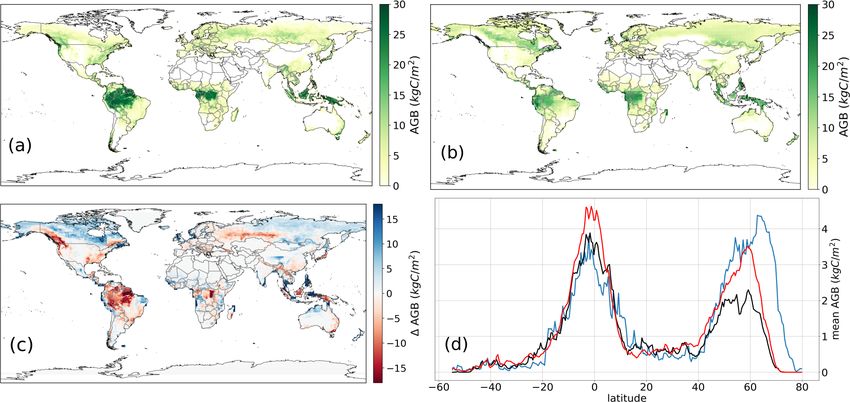
M. Drüke et al.: CM2Mc-LPJmL                                                                                                  4121

Figure 1. Schematic overview of CM2Mc-LPJmL and the most important variables exchanged between LPJmL5, FMS and AM2.

tributed onto the MPI tasks. As this LPJmL5 grid is not            ration (Monteith, 1965). The Penman–Monteith approxima-
compatible with the FMS grid exchange framework, a small           tion also accounts for additional parameters, such as hu-
wrapper library was developed for the data exchange be-            midity, that were previously not available in the stand-alone
tween LPJmL5 and FMS domains. The wrapper library is               LPJmL5 model (Fig. 2):
called for the ingoing and outgoing data, and the time over-
                                                                              dqsat                    ρa Cp (es0 −ea )
head for this data exchange is negligible. The coupler func-                   dT (Rn − G) + 86 400 ·       τaν
tion as well as the wrapper library are part of the LPJmL5         Lv ET0 =           dqsat         τs
                                                                                                                          ,    (1)
                                                                                       dT + γ (1 + τaν )
distribution.
                                                                   where Lv is the volumetric latent heat of vaporization of
2.3.2   New canopy module                                          2453 MJ m−3 , ET0 is the evapotranspiration (in m d−1 ), dqdTsat
                                                                   is the slope of the vapor pressure curve (in kPa ◦ C−1 ), Rn
The stand-alone version of LPJmL5 does not calculate the           is the net radiation at the surface (in MJ m−2 d−1 ), G is
essential coupling variables, canopy temperature and humid-        the soil heat-flux density (in MJ m−2 d−1 ), 86 400 is the
ity, which is remedied in the coupled configuration via the        conversion factor from seconds to daily values, ρa is the
addition of a new canopy module. In this new module, the           air density (in kg m−3 ), Cp is the specific heat of dry air
canopy humidity and canopy temperature and some further            (1.013 × 10⁻³ MJ kg−1 ◦ C−1 ), es0 is the saturated water va-
quantities linked to those variables are calculated (Fig. 2). In   por pressure (in kPa), ea is the actual water vapor pressure (in
this setting, the canopy layer corresponds to the lower bound-     kPa), τaν is the bulk surface aerodynamic resistance for water
ary for the temperature in the atmosphere. The atmospheric         vapor (in s m−1 ) and τs is the canopy surface resistance (in
diurnal cycle as well as the seasonal changes depend on the        s m−1 ). γ is the psychrometric constant (in kPa ◦ C−1 ) and is
surface energy balance. The canopy humidity, on the other          calculated as follows:
hand, is the lower boundary for the atmospheric humidity                Cp P
and, hence, sets the moisture content and the amount of pre-       γ=          = 0.000665P ,                                    (2)
                                                                         µλ
cipitation in the atmosphere as well as the potential for evap-
otranspiration at the surface. A schematic overview of the         where P is the atmospheric pressure at the surface (in kPa),
different calculation steps is provided in Fig. 3.                 λ is the latent heat of vaporization of 2.45 MJ kg−1 and µ is
   In the stand-alone version of LPJmL5, climatic input is         the ratio of molecular weight of water vapor to dry air (which
prescribed; therefore, calculations of processes and fluxes,       is 0.622). ET0 is presented here in the general daily form but
such as evapotranspiration, do not feed back to the atmo-          is applied to the model on the sub-daily timescale; thus, it is
sphere. In the coupled version, however, a small perturba-         divided by the number of time steps per day (in the current
tion in a positive feedback loop can influence the climate and     version 24).
push the process towards an even larger perturbation. Thus,           Equation (1) uses the canopy surface resistance τs , which
special attention has to be given to ensure the stability of the   is the reciprocal of the non-water-stressed canopy conduc-
model by either ignoring the feedback and implementing a           tance gp (in mm s−1 ). gp was also slightly changed, com-
simple, empirical and stabilizing relationship or by increas-      pared with Schaphoff et al. (2018b), in order to include cli-
ing the complexity of the implementation, in order to get a        mate feedbacks. Following Medlyn et al. (2011), we included
more realistic representation of the vegetation embedded in        a PFT-specific stomatal conductance parameter g1 (as de-
the Earth system. The latter was done in CM2Mc-LPJmL by            fined in De Kauwe et al., 2015) and the vapor pressure deficit
replacing the former simple Priestley–Taylor approach for          (D).

calculating potential evapotranspiration ET0 with the more                1000                    g1 Adt
complex and process-based Penman–Monteith evapotranspi-            gp =         = g0 + 1.6 1 + √            ,                 (3)
                                                                           τs                      D pa

https://doi.org/10.5194/gmd-14-4117-2021                                              Geosci. Model Dev., 14, 4117–4141, 2021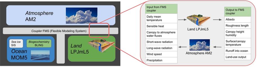
4122                                                                                           M. Drüke et al.: CM2Mc-LPJmL

Figure 2. Schematic overview of the new canopy module.

where g0 (in mm s−1 ) is a PFT-specific minimum canopy
conductance scaled by FPC, occurring due to processes other
than photosynthesis. pa is the ambient partial pressure of
CO2 (in Pa), Adt denotes the daily net daytime photosynthe-
sis and 1000 is the unit conversion factor from millimeters
to meters. D (in Pa) can be obtained by the canopy humidity
qca and the saturation humidity qsat :
D = qsat − qca .                                            (4)
While the new potential evapotranspiration is calculated at
the sub-daily time step, the non-water-stressed canopy con-
ductance is calculated at a daily time step, due to the daily
calculation of the photosynthesis in LPJmL5. As climate data
from FMS are available on a sub-daily basis, the photosyn-
thesis routine uses a diurnal average of air temperature and
photosynthetic active radiation.
   The newly calculated potential evapotranspiration, ac-
counting for gp , is then also used in several LPJmL5 rou-
tines (e.g., bare soil evaporation or interception) instead of
the equilibrium evapotranspiration (Eq ), which was based on
the Priestley–Taylor formula (Schaphoff et al., 2018b).
   As a next step, we calculate the water-stressed transpira-
tion Etr , using the supply–demand functions of LPJmL5 as
follows: the demand is calculated by the newly implemented
potential evapotranspiration (Eq. 1, corrected by the frac-        Figure 3. Schematic overview of the most important processes to
tion used for interception), and the supply is driven by ver-      determine the canopy humidity. Yellow denotes newly implemented
tical root distribution and phenology (as in Schaphoff et al.,     processes in the new canopy layer in LPJmL5, green denotes inter-
2018b). The initial transpiration is then a function of the min-   nal LPJmL5 calculations and blue denotes input, provided by the
imum of supply and demand for water. Following this, tran-         FMS coupler. Daily processes are indicated by a dotted line, and
spiration is subtracted from the various soil layers, depending    processes operating at a sub-daily time step are shown using a solid
                                                                   line.
on water availability. If the available water is not sufficient,
transpiration decreases. The adjusted transpiration is conse-
quently used in an inverse version of the Penman–Monteith

Geosci. Model Dev., 14, 4117–4141, 2021                                              https://doi.org/10.5194/gmd-14-4117-2021
M. Drüke et al.: CM2Mc-LPJmL                                                                                                  4123

formula in order to calculate the actual canopy conductance,        is important for the FMS coupler, are calculated at a sub-
linked to transpiration gtr .                                       daily time step. Equation (9) is based on Milly and Shmakin
   The total canopy conductance is additionally influenced          (2002) and is derived in Appendix C.
by the conductance of soil evaporation (ge ) and plant in-             It was also necessary to implement the calculation of
terception (gi ). Therefore, we use a simple approach taking        surface/canopy temperature within LPJmL5, which required
the maximum rainfall interception conductance (GIMAX =              major adaptions to the energy cycle in LPJmL5. The stand-
10 mm s−1 ) into account and considering the fraction of rain-      alone LPJmL5 model calculates the temperature of different
fall i stored in the canopy of a biome-dependent rainfall           soil layers by employing a temperature transport scheme and
regime (Gerten et al., 2004):                                       considering air temperature as climatic input. In CM2Mc,
                                                                    however, the energy balance is calculated on the surface and
gi = GIMAX · i · Pr/ET0 · fv ,                               (5)    then passed to the coupler and the atmosphere. Therefore, we
                                                                    had to implement this energy balance analogously in the cou-
where fv is the vegetated grid cell fraction, and Pr is the daily
                                                                    pled version of LPJmL5. While this surface temperature de-
precipitation. Pr and ET0 are applied in millimeters per sec-
                                                                    pends on several inputs from the coupler, such as radiation,
ond (mm s−1 ) here. The soil-evaporation conductance is cal-
                                                                    it also uses several variables connected to the water cycle
culated for the non-vegetated area of a grid cell and depends
                                                                    in LPJmL5 (evaporation, sublimation and melted water). As
on the maximum soil conductance (GEMAX = 10 mm s−1 ;
                                                                    our approach does not account for a height-dependent canopy
Huntingford and Monteith, 1998) and an empirical scaling
                                                                    temperature, we used the surface temperature as an approxi-
factor for the dependency of soil-evaporation conductance on
                                                                    mation for the canopy temperature, which is needed to calcu-
soil water status (α0 = 10, Zhou et al., 2006):
                                                                    late canopy humidity and evapotranspiration. Hence, surface
ge = (1 − fv ) · GEMAX · exp(α0 · (wevap − 1)),              (6)    temperature and canopy temperature are assumed to be the
                                                                    same, following the approach in the LaD model (Milly and
where wevap is the soil water content relative to the water-        Shmakin, 2002).
holding capacity available for evaporation defined for a cer-          The soil temperature is still important for internal pro-
tain soil depth (Schaphoff et al., 2018b). Both conductances        cesses in LPJmL, such as permafrost, but it is not needed
are calculated at a daily time step.                                in the coupler to calculate fluxes from the land to the atmo-
   We then calculate the total canopy conductance gc by             sphere. The calculation of heat transfer in the soil layers uses
adding gtr , gi and ge and using τaν following Milly and            the heat-convection scheme as in stand-alone LPJmL5 model
Shmakin (2002).                                                     (Schaphoff et al., 2018b) by taking the air temperature into
                                                                    account, which highly depends on the canopy temperature.
                         ρa
gc =                                         ,               (7)    Both temperature calculations, for the surface/canopy tem-
             1
       (gtr +gi +ge )   + (1 − βph ) · τaν                          perature and for the soil temperature, operate at the fast time
                                                                    step.
where βph is the water available for photosynthesis:                   In order to calculate the surface/canopy temperature

                Wr
                                                                   within LPJmL5, we employed a simple energy balance for-
βph = min              , 1   ,                               (8)    mulation for the incremental change in temperature 1T for
            0.75 · Wr∗
                                                                    each time step (adapted from Milly and Shmakin, 2002):
with Wr as the actual soil water and Wr∗ as the maximum                    Rn − m · LEf + ET · LEv − Qsn − H
available soil water. The increment of the canopy humidity          1T =                                     ,                 (10)
                                                                                         Cs · 1t
qca per time step is then calculated as follows, using gc :
                                                                    where m is the melted ice transformed to water (in
                       dqsat        dT                              kg m−2 s−1 ), LEf is the latent heat of the conversion of ice
dqca   ET − qflux +          · gc ·
     =                  dT          dt ,                     (9)    into water (in J kg−1 ), LEv is the latent heat of the con-
 dt             dqflux                                              version of water into vapor (in J kg−1 ), Qsn is the energy
                 dqca + gc
                                                                    released by snow (in W m−2 ), H is the sensible heat pro-
where qflux is the water flux from the canopy layer to the          vided by the FMS (in W m−2 ), Cs is the heat capacity of the
atmosphere, provided by the FMS coupler; dT   dt is the gradi-      soil (in J kg−1 ) and 1t is the fast time step duration (in s).
ent of the surface temperature over time; and ET is the fi-         Rn is used here in watts per square meter (W m−2 ). While
nal evapotranspiration, consisting of transpiration, evapora-       the temperature is calculated individually for each stand,
tion, interception and sublimation from surface or vegetation       a weighted average over all stands within one grid cell is
into the canopy layer. For the calculation of ET, we used           used in the humidity calculation and passed to the coupler.
the Penman–Monteith equation (Eq. 1), now applying the              The heat balance of snow is calculated as performed for the
total water-stressed canopy conductance gc (Eq. 7). dq   flux
                                                       dqca is      soil layers (see Schaphoff et al., 2018b), where snow tem-
the evaporation–humidity gradient. The total canopy conduc-         perature changes (1Tsnow ) depend on the thermal conduc-
tance and the final increment of the canopy humidity, which         tivity (λsnow = 0.2 W m−2 K−1 ) and heat capacity (Csnow =

https://doi.org/10.5194/gmd-14-4117-2021                                              Geosci. Model Dev., 14, 4117–4141, 2021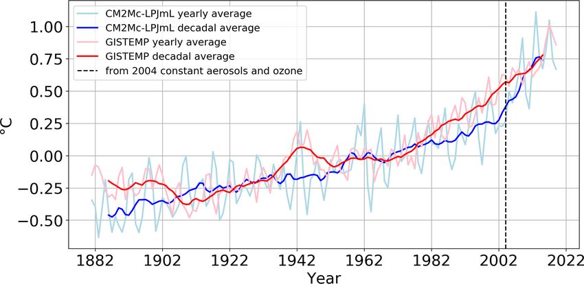
4124                                                                                        M. Drüke et al.: CM2Mc-LPJmL

630 000 J m−3 K−1 ) of snow as follows:                           using a simplified approach and will be replaced with the Par-
                                                                  allel Ice Sheet Model (PISM, Winkelmann et al., 2011) in the
1Tsnow   λsnow Tair + Tsoil[0] − 2 · Tsnow
       =       ·                           .              (11)    future. For now, Antarctica is assigned the ice soil type and a
 1t      Csnow         1zsnow 2                                   constant albedo of 0.7. The temperature balance is calculated
The heat flux from snow (Qsnow ) is calculated as follows:        as on the other continents.
                                                                     In the stand-alone LPJmL5 model, sublimation is sub-
                    (Tsnow − 1Tsnow )                             sumed by a constant global value of 0.1 mm d−1 , likely un-
Qsnow = λsnow ·                       ,                   (12)
                          zsnow                                   derestimating the sublimation at high latitudes. Especially
where zsnow is the snow depth, Tair is the air temperature and    in wintertime, we do not expect much evapotranspiration;
Tsoil[0] is the soil temperature of the first layer.              hence, the sublimation changes with meteorological condi-
                                                                  tions and becomes an important process. For this reason, we
2.3.3     Albedo and roughness length                             implemented the calculation of sublimation Es using the for-
                                                                  mula from Gelfan et al. (2004):
Albedo (β), the average reflectivity of the grid cell, is cal-
culated as in Schaphoff et al. (2018b), based on a first im-      Es = (0.18 + 0.098u)(es − ea ),                            (16)
plementation by Strengers et al. (2010) and later improved
                                                                  where u is the wind speed (in m s−1 ) from the coupler, es is
by considering several drivers of phenology by Forkel et al.
                                                                  the saturated vapor pressure (in mbar) and ea is the air vapor
(2014):
                                                                  pressure (in mbar).
        nX
         PFT                                                         Furthermore, the first test runs of the coupled models
β=             βPFT · FPCPFT                                      proved the need to tune some LPJmL5 PFT-specific parame-
      PFT=1                                                       ters: we increased the effective rooting depths of the tropical
  + Fbare · (Fsnow · βsnow + (1 − Fsnow ) · βsoil ),      (13)    tree PFTs to 2.3 m in order to counter a negative AM2 pre-
                                                                  cipitation bias in northern South America. Therefore, we in-
where the albedo for bare soil βsoil is defined as 0.3, and the   creased the β value of each tropical tree PFT, describing their
albedo for snow βsnow is defined as 0.7. βPFT is calculated for   vertical fine-root distribution in the soil column from 0.96 as
each PFT depending on the foliage projective cover (FPC)          in Schaphoff et al. (2018b) to 0.99 in this study.
and the stem, litter and leaf albedo of the respective PFT. The
value for each parameter is as in Schaphoff et al. (2018b).       2.4   Model setup and forcing
Fsnow and Fbare are the snow coverage and the fraction of
bare soil, respectively. Water bodies such as lakes and rivers    In the stand-alone version, as well as in the coupled version,
have a constant albedo value of 0.1.                              LPJmL5 is forced with gridded soil texture data (Nachter-
   Roughness length z0 m is calculated according to Strengers     gaele et al., 2009). Global atmospheric CO2 values are from
et al. (2010):                                                    Mauna Loa station data (Le Quéré et al., 2015) and land-use
                   r !                                            information is from Fader et al. (2010). The SPITFIRE fire
                      1                                           module (Thonicke et al., 2010) requires human population
z0 m = zb exp −                                            (14)
                     d                                            density as input, which is taken from Goldewijk et al. (2011),
                                                                  as well as lightning flashes, which are taken from the Opti-
and                                                               cal Transient Detector (OTD) and Lightning Imaging Sensor
      nX
       PFT
                FPCi                                              (LIS) satellite product (Christian et al., 2003). In the coupled
d=                 2 ,                                (15)    LPJmL5 version, we activated permafrost, the new phenol-
      i=1
              ln izb                                              ogy and SPITFIRE using the vapor pressure deficit as the fire
                  z0 m
                                                                  danger index (Drüke et al., 2019). The nitrogen cycle, which
where zb is the height of the boundary layer under stable con-    is part of LPJmL5 (Von Bloh et al., 2018), was deactivated in
ditions, set to 100 m (Ronda et al., 2003); z0i m is the PFT-     this study. Running in the coupled model, LPJmL5 receives
specific roughness length; and FPCi is the foliage projective     climatic input as, for instance, temperature, precipitation and
cover of each PFT, respectively. The coupler uses the rough-      radiation from the coupler interactively.
ness length to calculate aerodynamic resistance and surface          For the stand-alone LPJmL5 spin-up, we used the climate
drag and provides these variables to the different sub-models     data (temperature and precipitation) from the Land Data As-
of the ESM.                                                       similation System (GLDAS; Rodell et al., 2004). The orig-
                                                                  inal data have a spatial resolution of 0.25◦ × 0.25◦ and a
2.3.4     Further changes in the coupled LPJmL5                   time step of 3 h. We regridded the data set to the 0.5◦ × 0.5◦
                                                                  LPJmL5 resolution and aggregated it to a daily time step. For
For a global model we also need to consider Antarctica,           the spin-up, we recycled data from the years 1948–1978 (the
which has not been part of the standard grid of the stand-        earliest years available in GLDAS). Short-wave and long-
alone LPJmL5 modeling configuration. It was implemented           wave radiation was used from the coupled model CM2Mc,

Geosci. Model Dev., 14, 4117–4141, 2021                                           https://doi.org/10.5194/gmd-14-4117-2021
M. Drüke et al.: CM2Mc-LPJmL 4125
where the vegetation has been calculated by LaD (Milly and Table 1. Overview of the simulation experiments conducted in this
Shmakin, 2002). study. All runs, except for pi-CM2Mc-LaD and LPJmL-offline, are
For the fully coupled model run, we used 20 CPUs for the performed with CM2Mc-LPJmL. Other forcings include aerosols,
land and atmosphere calculations and 8 CPUs for the ocean, non-CO2 greenhouse gases, ozone and the solar constant. In the
totaling 28 CPUs. With these settings, 1 model year needs case of non-transient simulations, these are kept constant at their
values from the year 1860. Land use can either be transient (i.e.,
roughly 30 min on the PIK HPC cluster (Xeon E5-2667v3
capturing historical changes) or be deactivated.
8C 3.2 GHz, Infiniband FDR14). The number of MPI tasks
is limited by the coarse resolution of the atmosphere grid.
Experiment CO2 Land use Other forcings
Parts of the atmosphere code can employ hybrid MPI and [ppm]
OpenMP parallelism, but computational costs for LPJmL5
remain unaffected. pi-Control 284 No Constant
TR 284–408 Transient Transient
2.5 Modeling protocol PNV 284–408 No Transient
LU-only 284 Transient Constant
pi-CM2Mc-LaD 284 No Constant
Soil carbon and vegetation biomass need timescales of hun- LPJmL-offline 284–408 Transient Transient
dreds to several thousand years to reach an equilibrium with
climate, which would require extremely long spin-up simula-
tions in the coupled model. Hence, we first produce a spin-up
for 5000 years with the more computationally efficient stand- performed for the years 1700–2018: one with transient, his-
alone LPJmL5 model, using climate input from GLDAS and torical climate but PNV conditions without land use (PNV
an earlier CM2Mc-LaD run. To bring vegetation, soil and experiment), and the other with transient land use but prein-
climate into a consistent equilibrium (stand-alone LPJmL5 dustrial climate (LU-only experiment).
spin-up and the restart files from CM2Mc using LaD), we Two additional simulation experiments are conducted that
subsequently perform a fully coupled run of 500 simula- did not use the 500-year coupled spin-up: to compare the per-
tion years under preindustrial conditions with land use de- formance of CM2Mc-LPJmL against the original CM2Mc
activated. The climate of this run is then used as forcing model under preindustrial conditions, we conduct a 200-
for another stand-alone LPJmL5 spin-up run of 5000 years, year run of the CM2Mc model using the original LaD
producing restart conditions much closer to the state of the land model (pi-CM2Mc-LaD) and compare it against pi-
coupled model. This multistep spin-up approach minimizes Control. Here, we use restart files provided with the CM2Mc
the time for the computationally expensive coupled model to modeling suite. We also perform a transient stand-alone
reach a stable state. LPJmL5 (LPJmL-offline) run with a deactivated nitrogen cy-
To account for changed dynamics in the coupled system, cle (Schaphoff et al., 2018b; Von Bloh et al., 2018) in order
the LPJmL5 spin-up is then followed by a coupled spin-up, to compare the results to CM2Mc-LPJmL.
which runs for 500 years under preindustrial and potential
natural vegetation (PNV, i.e., without land use) conditions 2.6 Model evaluation
in a fully coupled setting. This fully coupled spin-up is the
starting point for the production runs (see Table 1), except Model performance is evaluated in terms of stability and his-
for the pi-CM2Mc-LaD and LPJmL-offline experiments. torical climate changes, and the results are compared to pi-
As a baseline run, we complete another 250 simulation CM2Mc-LaD runs, LPJmL5 stand-alone and observational
years under preindustrial PNV conditions in addition to the data. Specifically, our simulation experiments (see Table 1)
500 simulation years of the coupled spin-up, resulting in 750 are evaluated as follows: to analyze the stability of CM2Mc-
simulation years with the same settings (pi-Control experi- LPJmL, we evaluate temperature and precipitation of the
ment). 500-year coupled spin-up run combined with the 250-year
The transient run (TR) with variable land use and forc- pi-Control run (750 years in total).
ings is performed for the years 1700 until 2018, using his- Climate biases in precipitation and temperature are eval-
torical land-use data from 1700 onward, prescribed as out- uated by comparing the TR experiment from 1994 to 2003
lined in Fader et al. (2010); the concentration of greenhouse with global evaluation data sets from ERA5 (Dee et al.,
gases, solar radiation, ozone concentrations and the amount 2011). During the years 1994–2003, all forcing in CM2Mc-
of aerosols in the atmosphere are kept constant at preindus- LPJmL is transient. Simulated biomass is evaluated by com-
trial conditions until 1860 and then vary according to his- paring aboveground biomass from the TR experiment with
torical data. From 2004 onward, solar radiation, ozone and the GlobBiomass gridded data set by Santoro (2018) and
aerosols are kept constant due to missing data. Santoro et al. (2020). GlobBiomass provides vegetation car-
Similar to the TR experiment, we conduct two more ex- bon for roughly the year 2010; hence, we compare it to av-
periments in order to investigate the impact of climate and erage model data from 2006 to 2015. The PFT distribution,
land-use change in CM2Mc-LPJmL separately. Both runs are a measure of vegetation cover, is evaluated using data from
https://doi.org/10.5194/gmd-14-4117-2021 Geosci. Model Dev., 14, 4117–4141, 20214126 M. Drüke et al.: CM2Mc-LPJmL
Li et al. (2018) and Forkel et al. (2019) and comparing these
data with results from the TR experiment for the years 2006–
2015.
The historical temperature increase is quantified by com-
paring the transient temperature increase between 1860 and
2018 of the TR experiment with GISTEMP data (Lenssen
et al., 2019). GISTEMP combines various measurements
from meteorological stations. To evaluate the impact of
changes in atmospheric forcing on the spatial distribution
of climate parameters and vegetation, results from the last
10 years of the pi-Control experiment are compared with re-
sults from 2006 to 2015 of the PNV experiment (Sect. S2).
For analyzing land-use sensitivity (without variability in the
atmospheric forcing), we compare the last 10 years of the pi-
Control and the years 2006–2015 of the LU-only experiment
against each other.
In the Supplement, we further provide a comparison of
the results of CM2Mc-LPJmL and CM2Mc-LaD, using an
average over the last 10 years of the pi-Control and the
pi-CM2Mc-LaD experiments (Sect. S3), as well as a com-
parison with Coupled Model Intercomparison Project Phase
5 (CMIP5) data (Taylor et al., 2012) and LPJmL5-offline
Figure 4. Time series of monthly mean global (a) temperature and
(Sect. S4).
(b) precipitation (blue lines), and the corresponding 10-year run-
As evaluation metrics, we used the normalized mean error ning means (orange lines) in the pi-Control experiment.
(NME; Kelley et al., 2013):
PN
|yi − xi | 3.1.1 Model stability
NME = Pi=1
N
, (17)
i=1 |yi − x|
The analysis of the model stability was based on the pi-
where yi is the simulated value in grid cell i, and xi is the Control experiment, which ran over 750 years in total (see
observed value in grid cell i. x is the mean observed value. Sect. 2.5 for details). Here, we evaluate temperature and pre-
The NME is one if the model is as good as using the data cipitation in terms of absolute values as well as the rate of
mean as a predictor, larger than one for worse performance change over time and the variability.
and zero for perfect agreement. We use this metric for the After the initial 300 years, the global temperature remains
evaluation of the performance of temperature, precipitation relatively stable at ca. 14.7 ◦ C over the remaining simulation
and aboveground biomass. period of 400 years with a slight drift of less than of 0.05 ◦ C
per 100 years (Fig. 4a). The interannual variability in this pe-
riod is ca. 0.1–0.2 ◦ C. The decreasing temperature over most
3 Results of the 750-year simulation period can be explained by the
energy uptake of the ocean, as deep ocean layers are not yet
The evaluation of the model performance is provided in in equilibrium. The average precipitation follows a similar
Sect. 3.1, and the impact of land-use change on the results of trend as temperature and reaches a relatively stable state at
the coupled CM2Mc-LPJmL model is analyzed in Sect. 3.2. around 2.88 mm d−1 after ca. 400 years, changing less than
0.01 mm d−1 over the remaining period (Fig. 4b). The inter-
3.1 Model performance annual variability is 0.01–0.02 mm d−1 .
Here, we evaluate the performance of CM2Mc-LPJmL 3.1.2 Temperature evolution over the historical period
against climate and biosphere observations by first looking
into the long-term stability of global mean surface tempera- The temperature evolution over the historical period (and
ture (referred to as temperature, hereafter) and precipitation hence the climate sensitivity to changes in atmospheric forc-
(Sect. 3.1.1) from the pi-Control experiment, before evaluat- ing) is evaluated by comparing the transient temperature in-
ing the historical temperature increase of the coupled model, crease in the 1880–2018 period of the TR experiment to
using the TR experiment results. Finally, a detailed analy- GISTEMP evaluation data (Lenssen et al., 2019). We further
sis of climate (Sect. 3.1.2 and 3.1.3) and vegetation cover evaluate the spatial impact of historical climate change with-
(Sect. 3.1.4) is provided, also based on the TR experiment. out land use by comparing the years 2006–2015 of the PNV
Geosci. Model Dev., 14, 4117–4141, 2021 https://doi.org/10.5194/gmd-14-4117-2021M. Drüke et al.: CM2Mc-LPJmL 4127
Figure 5. Yearly and decadal global mean temperature anomaly
(relative to the 1951–1980 reference period) of the TR experiment
of CM2Mc-LPJmL compared to GISTEMP data from 1880 to 2018.
Note that, from 2004 on, only greenhouse gas forcing remains,
while aerosols, solar radiation and ozone are set to their correspond-
ing 2003 values.
experiment with the last 10 years of the pi-Control experi-
ment in the Supplement (Sect. S2).
The temperature evolution over the historical period from
1880 to 2018 is well captured as compared to GISTEMP
evaluation data (Fig. 5). Throughout the displayed period,
temperature anomalies are negative before the year 1962 and
remain positive afterwards, as climate change is accelerating.
While the temperature anomalies are slightly underestimated
between 1980 and 2010, GISTEMP and the TR experiment
both have an average global temperature increase of 0.75 ◦ C
in the year 2018 relative to the reference period from 1951 to
1980. Our results are also within the range of CMIP5 models Figure 6. (a) Global mean surface temperature of the TR experi-
(Kattsov et al., 2013; Taylor et al., 2012, Sect. S4). The inter- ment over the 1994–2003 period. (b) Surface temperature anoma-
annual variability in CM2Mc-LPJmL is ca. 0.5 ◦ C and, thus, lies between CM2Mc-LPJmL (TR) and ERA5 data over the 1994–
larger than in the GISTEMP data (ca. 0.25 ◦ C), although the 2003 period. (c) Latitudinal temperature mean of TR (red line) and
decadal changes are smaller in CM2Mc-LPJmL. ERA5 data (blue line) for the 1994–2003 period.
In the PNV experiment, climate change is also well cap-
tured, but it is weaker than when land use is included in the
model (Fig. S5). Large differences between CM2Mc-LPJmL and ERA5 are
also visible for mountainous areas, where the temperature
3.1.3 Surface temperature evaluation bias is partly due to the coarse resolution of the model not
adequately capturing the orographic influence of most moun-
Basic climate patterns are well captured in the annual mean tain ranges on climate (e.g., the Andes or Himalaya).
surface temperature (Fig. 6a), as temperatures are increasing While the seasonal cycle is usually well captured in
from polar temperatures of below −10 ◦ C towards the Equa- CM2Mc-LPJmL, especially in Antarctica a strong seasonal
tor with a maximum of ca. 25–30 ◦ C in the tropics. Desert temperature bias is partly balanced out in the annual mean
regions are usually warmer, whereas mountainous regions temperature. The temperature over Antarctica is largely over-
are colder than the surrounding area. In the high latitudes, estimated during the Southern Hemisphere summer, whereas
ocean cells are usually a bit warmer than land cells due to the it is underestimated during the Southern Hemisphere winter
ocean’s ability to store heat. (Figs. S1, S2).
Between 1994 and 2003, the average global temperature The latitudinal distribution of modeled mean temperature
is 15.6 ◦ C compared with 14.3 ◦ C in the ERA5 data set with between 1994 and 2003 (Fig. 6c) shows similar values to
a NME of 0.16. While the temperatures in the tropics and ERA5 data from high- to midlatitudes in the Northern Hemi-
temperate zone are slightly overestimated (by ca. 1 ◦ C), the sphere, but a slight overestimation in parts of the temperate
poles and the boreal zone show a large negative temperature zone and the tropics (between 70◦ S and 40◦ N). Specifically,
bias (up to −10 ◦ C) (Fig. 6b). The Southern Ocean has a the cold bias in the boreal zone leads to a slight underestima-
significant positive temperature bias (ca. 3 ◦ C on average). tion of temperature between 60 and 90◦ N.
https://doi.org/10.5194/gmd-14-4117-2021 Geosci. Model Dev., 14, 4117–4141, 20214128 M. Drüke et al.: CM2Mc-LPJmL
compared with 0.16 for temperature (Fig. 7b). The biases are
strongest at the Equator with an apparent shift of the ITCZ.
While precipitation in the Pacific is underestimated directly
at the Equator, it is overestimated north and south of the
Equator (Fig. 7b). Moreover, northern South America shows
a large negative precipitation bias.
The seasonal patterns (Figs. S3, S4) confirm the impre-
cise modeling of the ITCZ, which remains north and south of
the Equator for a large part of the year and passes the Equa-
tor region relatively swiftly. While precipitation south of the
Equator is overestimated, it is underestimated north of it.
The latitudinal annual mean precipitation between 1994
and 2003 (Fig. 7c) compares well with observations, display-
ing the global precipitation maximum in the tropics, local
minima in the subtropics and very low values at high lati-
tudes. The tropics, however, show a shifted maximum. While
the ERA5 global precipitation maximum over the Pacific
is at ca. 10◦ N and a local smaller maximum is at −10◦ S,
CM2Mc-LPJmL models the global maximum at roughly
−10◦ S and a smaller local maximum at ca. 10◦ N. The differ-
ence between the two maxima is less pronounced compared
with ERA5.
The comparison of the results of CM2Mc-LPJmL with the
original pi-CM2Mc-LaD model shows similar biases in rela-
tion to ERA5 for both model versions. Neither of the models
precisely captures the behavior of the ITCZ, especially over
the Pacific. Both models also show a large dry bias in north-
ern South America (Fig. S6).
3.1.5 Vegetation cover and biomass
Figure 7. (a) Global mean precipitation of the TR experiment
for the 1994–2003 period. (b) Precipitation anomalies between
CM2Mc-LPJmL (TR) and ERA5 data over the 1994–2003 period. While the evaluation of temperature and precipitation is per-
(c) Latitudinal temperature mean of TR (red line) and ERA5 data formed for the years 1994–2003, we compare average model
(blue line) over the 1994–2003 period. results for aboveground biomass (AGB) and the dominant
PFT for the years 2006–2015 due to availability of evalua-
tion data.
The comparison of CM2Mc-LPJmL (pi-Control) and pi- Simulated AGB shows a good pattern overall, with the
CM2Mc-LaD (as in Galbraith et al., 2011) shows that sim- largest values in the tropics, decreasing biomass in the sub-
ilar biases in relation to ERA5 are present in both model tropics, and a local maximum in the temperate and bo-
versions. For example, both model versions slightly overesti- real zone (Fig. 8d). In vegetation-free areas, such as deserts
mate global temperature (Fig. S6). The strong regional biases or polar regions, simulated AGB is zero or very close to
compared with ERA5 data are also present in both model se- zero (less than 200 g C m−2 ). When comparing AGB against
tups (Fig. S6) and are, therefore, not due to the implementa- GlobBiomass (Fig. 8a), spatial differences emerge (Fig. 8c).
tion of LPJmL5. While simulated AGB is slightly overestimated in boreal
North America and Asia, it is underestimated in the Eu-
3.1.4 Precipitation evaluation ropean temperate zone and in Scandinavia, extending into
eastern Europe and West Siberia. In most of the other tem-
The spatiotemporal pattern of global precipitation is well perate, Mediterranean-type and subtropical regions, AGB
simulated with a global average of 2.86 mm d−1 and a maxi- matches the observed values. In the tropics, AGB is overes-
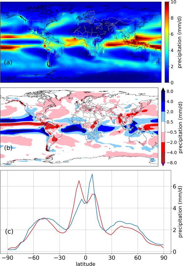
mum of up to 10 mm d−1 in the tropics close to the Intertropi- timated in semiarid regions, whereas wet tropical rainforests
cal Convergence Zone (ITCZ; Fig. 7a). Regions with little to are mostly underestimated, especially the eastern Amazon.
no vegetation, such as deserts and polar areas, receive very AGB shows good agreement in the seasonally dry Cerrado
little precipitation throughout the year. region in South America but appears to be overestimated
Precipitation biases with respect to ERA5 data are, how- in the Caatinga in northeastern Brazil. In central Australia,
ever, stronger than temperature biases, with an NME of 0.50 AGB matches observations but is overestimated in the north-
Geosci. Model Dev., 14, 4117–4141, 2021 https://doi.org/10.5194/gmd-14-4117-2021M. Drüke et al.: CM2Mc-LPJmL 4129 Figure 8. (a) Mean global aboveground biomass of GlobBiomass evaluation data. (b) Mean global aboveground biomass of CM2Mc- LPJmL (TR) over the 2006–2015 period. (c) Difference in the aboveground biomass between CM2Mc-LPJmL and GlobBiomass evaluation data. Blue (red) denotes an overestimation (underestimation) of biomass by CM2Mc-LPJmL. (d) Latitudinal sum of aboveground biomass from CM2Mc-LPJmL (blue line, R 2 = 0.64, NME = 0.56), stand-alone LPJmL5 (black line, R 2 = 0.94, NME = 0.35) input data and Glob- Biomass evaluation data (red line). ern part of the continent and underestimated in the southeast- ern part (Fig. 8c). Figure 8d compares the latitudinal mean of CM2Mc- LPJmL and LPJmL-offline with the evaluation data. LPJmL- offline shows better performance than the coupled model, with a smaller NME (0.35 vs. 0.56) and a better R 2 (0.94 vs. 0.64). While both models underestimate biomass in the tropics, biomass in the boreal zone is overestimated by CM2Mc-LPJmL and underestimated by the stand-alone LPJmL5 model compared with GlobBiomass. The LPJmL5 stand-alone version is forced by a reanalysis climatic input with a 0.5◦ spatial resolution, and the model is calibrated to this specific climate conditions; therefore, better model per- formance is expected. Modeled biomass is also within the range of CMIP5 models (Fig. S7). The geographic distribution of dominant PFT cover in CM2Mc-LPJmL follows the spatial pattern of the biomass distribution (Fig. 9a). The tropics are mostly dominated by the evergreen tree PFT. In the tropical savanna areas, the trop- ical deciduous tree PFT dominates, along with the C4 -grass Figure 9. (a) The dominant PFT for each cell, modeled by CM2Mc- PFT. The temperate zone is dominated by land use with some LPJmL. Cells with more than 50 % land use are masked using gray. summergreen trees – most common in areas such as Europe. Cells with less than 200 g C m−2 are shown using white. Full names The boreal zone is correctly covered by boreal needle-leaved of PFTs can be found in Appendix B. (b) The sum of squares errors and boreal summergreen trees, and the tundra zone is covered of ESA CCI land cover for each PFT in each cell. Blue areas have a with polar grasses. To better visualize the model error for the small error, and red areas have a large error. The error shown here is PFT distribution, we produced an error map that consists of absolute; hence, areas with a low PFT cover for both model and the sum of the square error for each PFT per cell (Fig. 9b). evaluation data are small compared with areas with a large PFT In tropical rainforests, the error with respect to the evalua- cover. tion data is relatively small. Drier savanna areas show a much https://doi.org/10.5194/gmd-14-4117-2021 Geosci. Model Dev., 14, 4117–4141, 2021
You can also read