Reservoir characterization and volumetric estimation of reservoir fluids using simulation and analytical methods

Reservoir characterization and
volumetric estimation of reservoir fluids
using simulation and analytical methods
B. K. Kurah, B. K., M. S. Shariatipour, and K. Itiowe

Final Published Version deposited by Coventry University’s Repository

Original citation & hyperlink:
Kurah, B.K., Shariatipour, M.S. and Itiowe, K., 2021. Reservoir characterization and
volumetric estimation of reservoir fluids using simulation and analytical methods: a case study
of the coastal swamp depobelt, Niger Delta Basin, Nigeria. Journal of Petroleum Exploration
and Production Technology, 11 (6), pp. 2347–2365.

DOI 10.1007/s13202-021-01206-1
ISSN 2190-0558

Publisher: Springer

Open Access This article is licensed under a Creative Commons
Attribution 4.0 International License, which permits use, sharing,
adaptation, distribution and reproduction in any medium or format,
as long as you give appropriate credit to the original author(s) and
the source, provide a link to the Creative Commons licence, and
indicate if changes were made. The images or other third party
material in this article are included in the article's Creative Commons
licence, unless indicated otherwise in a credit line to the material. If
material is not included in the article's Creative Commons licence and
your intended use is not permitted by statutory regulation or exceeds
the permitted use, you will need to obtain permission directly from
the copyright holder. To view a copy of this licence,
visit http://creativecommons.org/licenses/by/4.0/.

Journal of Petroleum Exploration and Production Technology (2021) 11:2347–2365
https://doi.org/10.1007/s13202-021-01206-1

 ORIGINAL PAPER-EXPLORATION GEOLOGY

Reservoir characterization and volumetric estimation of reservoir
fluids using simulation and analytical methods: a case study
of the coastal swamp depobelt, Niger Delta Basin, Nigeria
B. K. Kurah1 · M. S. Shariatipour1 · K. Itiowe2

Received: 19 November 2020 / Accepted: 31 May 2021 / Published online: 15 June 2021
© The Author(s) 2021

Abstract
Suites of wireline well logs and three-dimensional (3D) seismic data were integrated to characterise the reservoir and
estimate the hydrocarbon in Otigwe field, coastal swamp depositional belt, Niger Delta. The 3D seismic data were used to
generate seismic sections through which fourteen faults and two horizons of interest were mapped across four wells. Depth
structural map generated from the mapped faults and horizons of interest shows that the trapping mechanism within the field
is fault-supported anticlinal structural trap. The four available wells were correlated using lithostratigraphic correlation to
establish two reservoir continuities (Reservoir A and B). The estimated reservoir fluid volume at surface condition using
reservoir simulation and modelling software is 59 MMstb for reservoir A and 25.70 MMstb for reservoir B. On the other
hand, the estimated reservoir fluid volume at surface condition using analytical method is 52.58 MMstb for reservoir A and
18.85 MMstb for reservoir B. Using reservoir simulation and modelling software, the average net-to-gross ratio and shale
volume for reservoir A range from 0.86 to 0.89 and 0.11 to 0.14, respectively, while for reservoir B the range is between 0.69
to 0.82 and 0.18 to 0.31, respectively. On the flipside using the analytical method, the average net-to-gross ratio and shale
volume for reservoir A is 0.78 and 0.22, respectively. The results from the volumetric estimation of reservoir fluids showed
close values using both methods and reservoir A is more prolific compare to B.

Keywords Characterization · Volumetric · Porosity · Permeability · Prolific

Introduction most significant region within the West African Continental
 Margin (Aizebeokhai and Olayinka 2011). Hydrocarbons
The Niger Delta Basin is ranked as one of the most prolific (oil and gas) in the Niger Delta are mostly extracted from
deltaic systems in the world with respect to hydrocarbon the Agbada Formation which is predominantly made up of
accumulations or reserves. This hydrocarbon province con- unconsolidated sandstone and shale. Since one of the ulti-
tains only one petroleum system called the Akata-Agbada mate goals of the oil and gas industry is to identify and char-
petroleum system (Tuttle et al. 1999). It is regarded as the acterise the reservoirs and estimate the volume of oil and
 gas in place, accurate delineation of structural traps on 3D
 seismic sections and effective well log analysis is required.
* K. Itiowe The application of well logs and 3D seismic for the charac-
 kiamukeitiowe@yahoo.com terisation and hydrocarbon volume estimation will aid in the
 B. K. Kurah decision-making process by identifying commercially viable
 biokpokurah@gmail.com zones for exploitation.
 M. S. Shariatipour Well log analysis and 3D seismic survey are two essen-
 seyed.shariatipour@coventry.ac.uk tial techniques used for reservoir characterisation in the
1 petroleum industry. These techniques help the geoscientist
 School of Energy, Construction and Environment, Faculty
 of Engineering, Environment and Computing, Coventry to have a better knowledge of the physical properties and
 University, Coventry, England, UK structural setting of the reservoir rock and the fluid con-
2
 Department of Earth Sciences, Arthur Jarvis University, tents. According to Weber (2012), when well log analysis
 Akpabuyo, Cross River State, Nigeria is integrated with 3D seismic interpretation, a detailed view

 13
 Vol.:(0123456789)

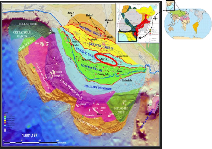
2348 Journal of Petroleum Exploration and Production Technology (2021) 11:2347–2365

Fig. 1  Location map of study area, indicated with the red oval (Oluwajanaet al. 2017; Tuttleet al. 1999)

of the subsurface geology and geophysical properties can Geological setting
be established. Since well logs are in depth, the top and
base of reservoirs can be mapped out and used to construct The Niger Delta is located in the Gulf of Guinea, on the
a subsurface structural and isopach/isobath map (Weber West Africa Margin and spreads all through the Niger Delta
2012). Depth measurement from well logs can be used to province between longitude 5 °E to 8 °E and 4 °N to 6 °N
convert two-way-time on a seismic section to depth. Res- (Tuttle et al. 1999) (Fig. 2). The Niger Delta Basin has three
ervoir fluid contents can be analysed through the use of formations which are the marine Akata, paralic Agbada and
well logs. Hence, fluid saturation within the porous media continental Benin Formations (Table 1). The Akata Forma-
can be calculated analytically using Archie’s formula, for tion is the primary source rock and is made up of marine
clean sandstone formation. According to Ajisafe and Ako shale (Doust and Omatsola 1990). The reservoir rock of the
(2013), it is more advantageous to integrate well log and Agbada Formation is made up of sandstone with shale inter-
seismic data for reservoir characterization than to use well calation. According to Kulke (1995), during the formation
data alone, because seismic data enables the extrapolation of the delta, there was equilibrium between the rate of sub-
and interpolation beyond and between sparse well controls. sidence and sedimentation. The depositional pattern of the
The vertical resolution obtained from well log data is excel- sediment was influenced by the tectonic setting and struc-
lent but has a poor areal resolution. On the other hand, 3D tural configuration of the terrain. The delta has prograded
seismic data provide high areal resolution, but with poor ver- south-westwards from the Eocene to Recent forming five
tical resolution (Ajisafe and Ako 2013). Accuracy of subsur- depositional belts at each stage of the formation (Doust and
face structural mapping and analysis would be significantly Omatsola 1990).
enhanced by integrating well logs and seismic data (Adejobi Rollover structures, multiple growth faults, antithetic
and Olayinka 1997; Barde et al. 2002). faults and collapsed crest structures are the main struc-
 Otigwe Field is located in the coastal swamp depositional tural features found in the Niger Delta (Fig. 2) (Tuttle
belt (depobelt) within the Niger Delta oil province, as shown et al. 1999). According to Evamy et al. (1978) and Stacher
in the red oval (Fig. 1).

 13

Journal of Petroleum Exploration and Production Technology (2021) 11:2347–2365 2349

Fig. 2  a Rollover structures with clay filled channel b Structure with multiple growth faults c Structure with antithetic faults and d collapsed
crest structures (Tuttle et al. 1999)

(1995), structural traps were formed during synsedimen- billion cubic metre are present in existing field. The seal
tary deformation of the petroleum bearing Agbada paralic rock in the Niger Delta is primarily interbedded marine
sequence. The structures become more complex towards shales within the Agbada formation. Three types of seals
the south with respect to gravitational instability of the are available: smearing of clay along faults, vertical seals
under compacted, over pressured Akata Formation (Tut- and interbedded sealing layers against which subsurface
tle et al. 1999). According to Doust (1989) hydrocarbons reservoir sands juxtapose because of faulting (Doust and
are trapped within the growth fault structure and about 4 Omatsola 1990).

Table 1  Age and Formations of the Niger Delta Sedimentary Basin (modified after Short and Stauble (1967))
Subsurface Surface outcrop
Youngest known Formation Oldest known age Youngest known age Formation Oldest known age
age

Recent Benin Fm Oligocene Holocene Alluvium Miocene?
 Ear. Holo. To Deltaic Plain
 Late Pleistoc Deposits
 Afam Shale Member Plio. / Pleist Benin Fm
Recent Agbada Fm Eocene Miocene Ogwashi - Oligocene
 Asaba Fm
 Eocene Ameki Fm Eocene
Recent Akata Fm Eocene L. Eocene Imo Shale Paleocene
 Equivalent not known Paleocene Paleocene Nsukka Fm Maestrich
 Maestrich Maestrich Ajali Fm Maestrich
 Campanian Mamu Fm Campanian
 Camp./ Mae Nkporo Sh Santonian
 Conia/ Santo Agwu Shale Turonian
 Turonian Ezeaku Shale Turonian
 Albian Asu River Gp Albian

 13

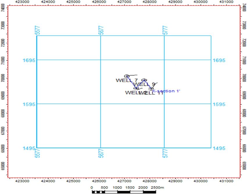
2350 Journal of Petroleum Exploration and Production Technology (2021) 11:2347–2365

Fig. 3  Seismic survey base map showing the location of four wells within the Otigwe field

Data set and methodology the picking of the horizons throughout all the inlines and
 crossline on the seismic sections. Check shot (time-depth
The data set consists of 3D seismic data (SEG-Y format), chart) data for well 2 were used to convert reservoir tops
well logs from four wells, well header, well deviation from from the well log in depth domain to two-way time domain
the four well and check shot (Time-Depth data). Two meth- on the seismic sections (Fig. 4). These logs were also used to
ods of data analysis were employed in this study. These are produce and display synthetic seismograms on the 3D seis-
the reservoir simulation/modelling software and analytical mic section for picking of horizons. The top of the horizons
method which involves using appropriate analytical formu- of interest which represents the reservoir top was adequately
lae Fig. 6. mapped and interpreted. The time and depth structural maps
 Reservoir simulation and modelling software was used in were produced to identify the area that was covered with
this study. The 3D seismic and well data set were imported hydrocarbon. The area was integrated with the thickness of
into the software. The wells are shown in the seismic survey the reservoir for the evaluation and estimation of the bulk
base map (Fig. 3). Non-reservoir zones, tops and base of the volume of hydrocarbon. The flow chart in Fig. 5 and Fig. 6
reservoirs were delineated from the well logs (using gamma, clearly illustrates the steps of the methodology.
density, sonic logs, etc.) and correlation of the reservoir top Shale contents are mostly present within the hydrocar-
and base were established. The reservoir simulation and bon-bearing sandstone reservoir. The presence of shale in
modelling software converted the 3D seismic data to series the productive zone has severe impact on the petrophysi-
of seismic sections consisting of inlines and crosslines, cal properties and can cause a reduction in the effective
through which picking of major and minor fault were car- and total porosity, as well as permeability. Moreover, it
ried out and interpreted using the appropriate tools on the also poses problem in the interpretation of wireline well
menu bar. This conversion process enables the identification logs and can affect proper and effective estimation of
of the horizon of interest (top of reservoir), which allow hydrocarbon or STOOIP (Moradi et al. 2016). Hence, its

 13

Journal of Petroleum Exploration and Production Technology (2021) 11:2347–2365 2351

Fig. 4  Survey check shot traveling time against depth for well 2

determination is crucial in solving the problem stated ear- Vsh = 0.083 23.7IGR − 1 Tertiary or younger rock (2)
 ( )
lier. According to Szabo (2011), various methods exist for
shale volume estimation, such as gamma ray log, sponta-
neous potential log or porosity-neutron log. In this study, Determination of total porosity
gamma ray log technique was used for the shale volume
estimation by first estimating the gamma ray index (IGR) Application of neutron-density log in porosity determina-
(Eq. 1). tion is the most commonly used technique in reservoir rock
 penetrated by a well (Ijasan, Torres-Verdin and Preeg 2013).
 GRlog − GRmin
IGR = Gamma ray Index = (1) The total porosity in hydrocarbon-bearing formation can be
 GRmax − GRmin determined using Eq. 3 (Gaymard and Poupon 1968 cited in
 Ijasan, Torres-Verdin and Preeg 2013).
where: GRlog represents gamma ray reading at the depth of
interest, GRmin and GRmax represent minimum and maxi- ma − b
 t = (3)
mum gamma ray values of the clean and shale formation, ma − f
respectively (Szabo 2011).
 Secondly, to obtain the realistic shale volume estima- Where, ma , b and f represent matrix,
tion without overestimating the content of shale (first-order
approximation: ­Vsh = ­IGR), a nonlinear relationship (for formation bulk and fluid density respectively
unconsolidated rock or chemically immature rock) was For sandstone lithology, ma =
 2.65 g
 , b is obtained
used in this study, by employing Eq. 2 (Szabo 2011). Since from density logand
 cm2

the Niger Delta sedimentary sequences are Tertiary rock or
younger rock, Eq. 2 was used.

 13

2352 Journal of Petroleum Exploration and Production Technology (2021) 11:2347–2365

Fig. 5  Flow chart of the methodology designed for this work

 f is obtained from literature because the lithological facies in the Niger Delta reservoirs
(for light crude in the Niger Delta) = 0.8 is made up of shaly-sand sequences.

 (4)
 ( )
 eff = total 1 − Vsh
Determination of effective porosity
 Where, eff , total and shale represent effective, total,
A porosity model and equation proposed for shaly-sand res- and shale porosity respectively ,
ervoirs by Al-Ruwaili (2007) were used for the determina-
tion of the effective porosity (Eq. 4). This was employed
 Vsh represents shale volume

 13

Journal of Petroleum Exploration and Production Technology (2021) 11:2347–2365 2353

Fig. 6  Methodological flow
chart demonstrating formula for
quantitative well log analysis
and interpretation, designed for
this work

Archie’s formula for water saturation determination where Sw represents water saturation level, Rw is the water
 resistivity, Rt is the formation resistivity (virgin zone) con-
Archie’s formula is the basic or elementary formula for com- taining the hydrocarbon, ∅ the total porosity of the reservoir.
puting water saturation for both the virgin and invaded zones Archie’s parameters a, m and n represent: tortuosity fac-
in the primary life of a given reservoir (Al-Awad 2001). For tor, cementation factor and saturation exponent.
a reservoir, the exactness or accuracy of the water saturation SW = Formation water saturation (fraction; obtained from
value depends on the exactness of the Archie’s parameters log data).
(a, m and n). In this work, Archie’s equation was used in
 (6)
 ( )
the determination of the water saturation in the virgin zone where; So = 1 − Sw(t)
(without mud filtrates) (Eq. 5).
 So = oil saturation.
 √
 a×R
Sw = n m w (5)
 � × Rt

 13

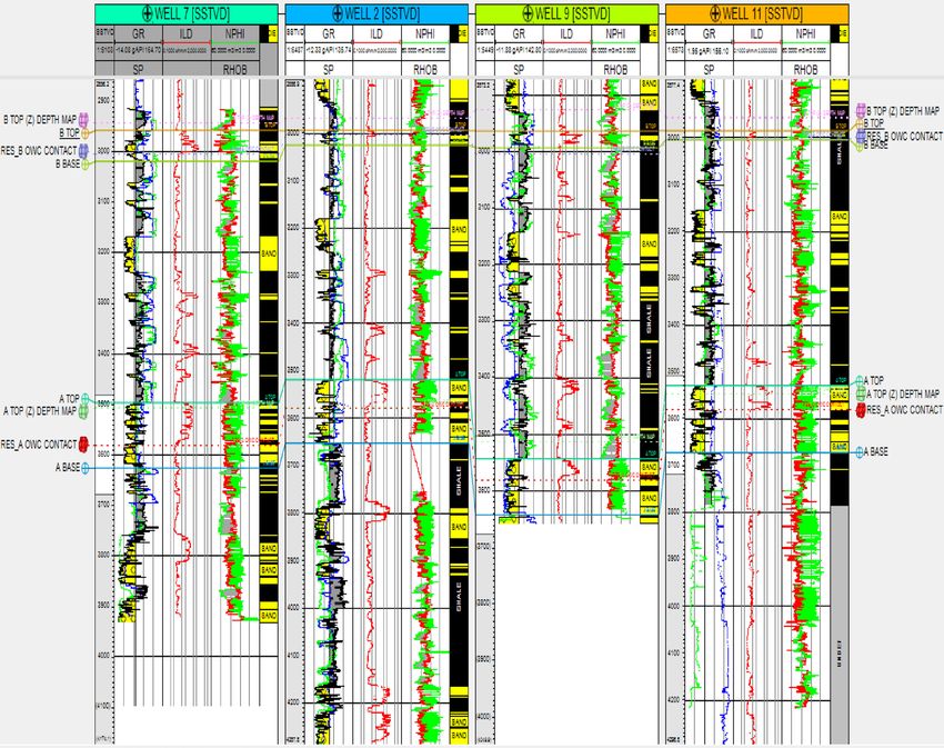
2354 Journal of Petroleum Exploration and Production Technology (2021) 11:2347–2365

Determination of Net‑To‑Gross Ratio Permeability determination

The net-to-gross ratio is the ratio of the total thickness Permeability is the ability of a porous medium to transmit
of the subsurface productive pay zone to that of the total fluid. In this study, the empirical expression for permeability
thickness of the subsurface reservoir interval for a vertical estimation by Awolabi, LongJohn and Ajienka (1994) was
well. Also, the net-to-gross ratio has a direct relationship employed. This method was used because it considers the
with the volume of shale as shown in Eq. 7 (Abbaszadeh unconsolidated reservoir sand within the Niger Delta hydro-
et al. 2003). When an entire reservoir interval is a pay zone, carbon province. The mathematical expression involves the
then net-to-gross is equal 1.0. Since the four available wells relationship between effective porosity, permeability and
in this study are all vertical wells and the entire sandstone irreducible water saturation as shown in Eq. (8).
reservoir or hydrocarbon-bearing interval contains interca-
 K(mD) = 26552 × 2 − 34540 × 2 × Swr (8)
 2
lation of shaly-layer, the net-to-gross ratio will therefore + 307
be less than unity (i.e. 1.0) and Eq. 7 was used for the
computation.
 Volumetric estimation technique
Net − To − Gross ratio = 1 − Vsh (7)
 The hydrocarbon volumes were estimated using the volumet-
 ric method (Eqs. 9, 10 and 11). Firstly, the hydrocarbon pore

Fig. 7  Stratigraphic correlation and well log analysis for the four wells

 13

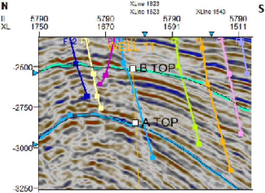
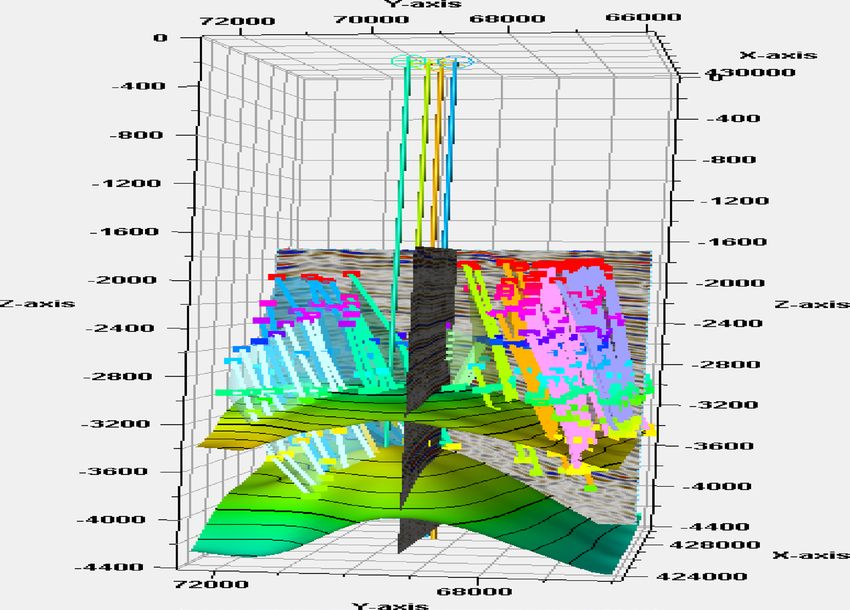
Journal of Petroleum Exploration and Production Technology (2021) 11:2347–2365 2355

volume was calculated using the reservoir simulation and
modelling software prior to the computation of the original
oil in place at surface condition by means of the formation
volume factor. The petrophysical parameters such as poros-
ity and water saturation, as well as net-to-gross ratio and
reservoir thickness were used to estimate the reservoir fluid
volume. These parameters were imputed into the following
formula.

 (9)
 ( )
HCPV = Vb × eff × NTG × 1 − Sw

 ( )
 vb × eff × NTG × 1 − Sw(t)
OOIP (t(STB) = STOIIP =
 Boi(p(t)
 (10)
 Vb = Bulk reservoir volume (bbl) = 7758Ah. Fig. 9  Interpreted seismic section (fault and horizon interpretation) of
 7758 = bbl\acre-ft. the Otigwe field
 A = Reservoir cross-sectional area; acres (obtained from
map data).
 Bo = Oil formation volume factor (1.2 bbls/stb for this
 h = Reservoir thickness (pay zone; ft) (obtained from log
 work).
data).
 ɸ = Formation porosity (fraction) (obtained from log
data).
 NTG = Net-to-Gross ratio.
 Results and discussion
 SW = Formation water saturation (fraction) (obtained
from log data)
 Stratigraphic correlation and interpretation

 (11) Lithostratigraphic correlation was used across the four wells
 ( )
Where;So = 1 − Sw(t)
 (Fig. 5). This was employed using the suite of wireline log
 So = oil saturation. signatures (i.e. gamma ray (GR), spontaneous potential

Fig. 8  Faults within the seismic
sections and tops of reservoir
A and B

 13

2356 Journal of Petroleum Exploration and Production Technology (2021) 11:2347–2365

(SP), bulk density (RHOB) and neutron-hydrogen porosity fresh formation water (Wei et al. 2014). Although, Passey
index (NPHI) logs). It provides general knowledge of the et al. (1990) stated that resistivity log signatures have less
subsurface stratigraphic sequences in the Otigwe Field. The application in shale identification because the mineralogical
correlated top and base of the sandstone reservoirs (yellow content in shale is not fully understood. Hence, the log tools
colours in the well logs) for reservoir A and B show the used for lithologic identification in this study were gamma
lateral continuity of the stratigraphic sequences in time and ray and spontaneous potential log signature. Having pro-
space. It establishes both the stratigraphic principle of lateral vided a distinction between the reservoir and non-reservoir
continuity of strata and Walther’s law of facies succession. rock with the suite of well logs, the hydrocarbon water con-
Reservoir A shows a slight uniform thickness across well 2, tacts across the four wells were delineated using resistivity
7 and 11, except well 9. On the other hand, reservoir B is and neutron-density log.
thinner in well 2, well 9 and well 11, except in well 7. Pinch- Gamma ray log reflects the amount of natural radioac-
out is deciphered to exist toward well 11. tive content (e.g. potassium, Uranium and Thorium) in rock
 (Etu-Efeotor 1997). Radiation emanates from these radio-
Well log analysis active elements. All rock contains radioactive content, but
 shale has the highest radioactive content compare to sand-
The interpreted well logs for the four wells indicate that the stone and limestone (Etu-Efeotor 1997). The result of the
reservoir rocks are generally unconsolidated sandstone with four logs in Fig. 5 shows that a deviation of the gamma ray
intercalation of interbedded shale sequences within each of log to the right of the shale baseline indicates shale layers
the reservoir interval. According to (Etu-Efeotor 1997), well whereas a deviation to the left of the shale baseline indicates
logs are basically used in the identification and characterisa- sandstone layers. This is because sandstones are free of shaly
tion of subsurface lithology and type of reservoir fluids (oil, material and has low radioactive contents. As the radioac-
gas and water). The lithologic sequences are delineated with tive material in the sandstone layer increases, the gamma
the aid of the gamma ray (GR) and spontaneous potential ray signature increases to the right. Hence, the increase is
(SP), whereas the unconsolidated nature of the reservoir proportional to the quantity of shale present. On the logs,
rock was delineated with the aid of the calliper log, indi- some intervals are found to be shaly-sand and sandy-shale.
cating the presence of caves. Also, the types of reservoir These intervals generally have radioactive material that falls
fluid were determined using resistivity (ILD), bulk density between clean sands and shales.
(RHOB) and neutron-porosity hydrogen index (NPHI) logs. Spontaneous potential log records the potential difference
Resistivity logs (ILD) can also be used to delineate lithol- between two electrodes and it is used to identify perme-
ogy, such that lower resistivity depicts shale or clay and able and impermeable zones (Dewan 1983). It is measured
medium–high resistivity depicts sand or gravel containing in millivolt, negative at the left and positive at the right.

Table 2  Petrophysical Well Number Vsh ɸt ɸeff K (mD) NTG Sw So h (m) hɸeffSo (m)
properties for the four wells in
reservoir A 2 0.11 0.24 0.21 103.10 0.89 0.21 0.79 50 8.30
 7 0.14 0.23 0.20 1678.22 0.86 0.32 0.68 73 9.93
 9 0.11 0.18 0.17 1199.02 0.89 0.30 0.70 31 3.69
 11 0.11 0.24 0.22 1783.28 0.89 0.21 0.79 50 8.69

Table 3  Petrophysical Well Number Vsh ɸt ɸeff K (mD) NTG Sw So h (m) hɸeffSo (m)
properties for the four wells in
reservoir B 2 0.16 0.24 0.21 138.14 0.84 0.41 0.59 12 1.49
 7 0.18 0.23 0.20 1841.58 0.82 0.21 0.79 43 6.79
 9 0.22 0.22 0.18 1649.18 0.78 0.22 0.78 22 3.09
 11 0.31 0.21 0.15 1499.55 0.69 0.55 0.45 13 0.88

Table 4  Simulated average of Reservoir Vsh ɸt ɸeff K (mD) NTG Sw So h (m) hɸeffSo (m)
the petrophysical properties of
Reservoir A and B A 0.12 0.22 0.20 1190.90 0.88 0.26 0.74 51 7.55
 B 0.22 0.23 0.18 1282.11 0.78 0.35 0.65 23 2.69

 13

Journal of Petroleum Exploration and Production Technology (2021) 11:2347–2365 2357

When a permeable zone is encountered, the spontaneous the absence of gas zones. Oil was found at a depth range
potential log signature deflects to the negative with respect of 3523 m to 3574 m in reservoir A and at a depth range of
to the impermeable zone (e.g. shale) while for an imper- 2976 m to 2999 m in reservoir B across the four wells using
meable zone, it deflects to the positive with respect to the the resistivity, neutron-porosity and bulk density logs. The
permeable zone (e.g. sandstone). In this study, the permeable presence of oil (green colour in the well logs) is indicated
and impermeable zones in the suites of four available well where there is separation between the neutron-porosity and
logs (Fig. 5) represent unconsolidated sandstone and shale, bulk density logs, in addition to the high resistivity, whereas
respectively. This affirms the lithological sequence identified below this oil zone is the water zone having low resistivity
in the Niger Delta (Short and Stauble 1967). (Fig. 7).
 The resistivity log was used in the identification of the The oil–water contact is the surface in a subsurface reser-
hydrocarbon-bearing reservoirs (unconsolidated sandstone voir separating the oil from the water. According to Okolie
reservoir). The resistivity of a rock or formation is a meas- and Ujanbi (2007), evaluation of oil–water contact within
ure of the ability to which it can resist or impede the flow the Niger Delta reservoir is difficult due to the presence of
of electric current. Formation water conducts electricity interbedded shale layers in the reservoir. In this study, the
because it is a function of salinity (Archie 1942; Bridge oil water contacts across the four wells in Fig. 5 were deter-
and Demicco, 2008). On the other hand, hydrocarbon fluids mined using the resistivity and combination of the neutron-
which are non-conductive increases the resistivity values, as porosity and bulk density logs. From the log analysis, the
the void spaces within the rock become fully saturated with oil water contacts across well 2, well 7, well 9 and well 11
hydrocarbon (oil or gas). The resistivity log signatures were in reservoir A were found to be 3570 m (11713 ft), 3570 m
observed to be evidently higher within the hydrocarbon- (11713 ft), 3576 m (11732 ft) and 3580 m (11745 ft), respec-
bearing zones than in the formation water saturated zone tively, whereas for reservoir B, the oil water contacts were
(Fig. 5). found to be 3008 m (9869ft), 3002 m (9849 ft), 2985 m
 In general, sandstones basically have a relatively low den- (9793 ft) and 3001 m (9846 ft), respectively. Estimation of
sity because of their relatively high porosity (Bridge and these oil water contacts is very important for reservoir char-
Demicco, 2008). The presence of gas within the pore spaces acterization and evaluation of original oil in place, since it
of the sandstone will lead to an extra density decrease; hence, aids in the determination of the oil section (Archer 1986;
there will be decrease in the neutron-porosity signature. This Adams 1993). This height/thickness of the oil section (from
decrease will cause the neutron-porosity signature to cross top of reservoir to the oil–water contact) was used in the
over the bulk density signature (Bridge and Demicco, 2008). estimation of the stock tank oil in place in this study.
The decrease in both the neutron-porosity and bulk density
signatures indicates the presence of gas in the reservoir, and Structural interpretation on seismic sections
this creates a large separation and forms a balloon shape
(Etu-Efeotor 1997). The gas effect is formed because gas Network of several normal faults was seen across the entire
comprises a smaller amount of hydrogen atoms compare seismic sections (Figs. 8 and 9). Fourteen (14) of these nor-
to oil and water (Etu-Efeotor 1997). Analysis of well logs mal faults were mapped and were found to trend northwest-
indicates the presence of oil zones in both reservoirs and southeast and dip southwest-southeast. It was observed that

Table 5  Petrophysical Well Number Vsh ɸt ɸeff K (mD) NTG Sw So h (m) hɸeffSo (m)
properties for the four wells
in reservoir A using analytical 2 0.22 0.26 0.22 1313.82 0.78 0.20 0.80 50 8.8
method
 7 0.22 0.26 0.20 1282.73 0.78 0.25 0.75 73 10.95
 9 0.22 0.19 0.15 893.23 0.78 0.08 0.92 22 3.64
 11 0.22 0.24 0.19 1250.444 0.78 0.11 0.89 50 8.46

Table 6  Petrophysical Well Number Vsh ɸt ɸeff K (mD) NTG Sw So h (m) hɸeffSo (m)
properties for the four wells
in reservoir B using analytical 2 0.22 0.20 0.23 1675.79 0.78 0.14 0.86 12 2.37
method
 7 0.22 0.30 0.23 1685.29 0.78 0.12 0.88 43 8.70
 9 0.22 0.23 0.18 1160.12 0.78 0.08 0.92 22 3.64
 11 0.22 0.26 0.20 920.20 0.78 0.57 0.43 13 1.12

 13

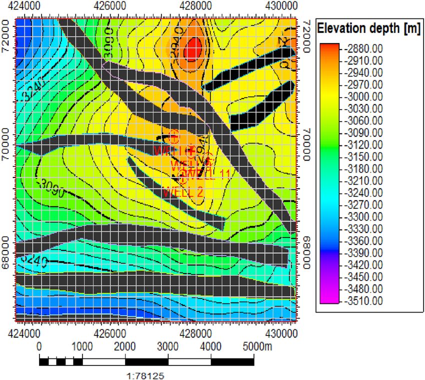
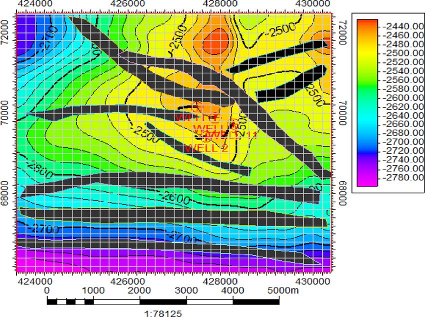
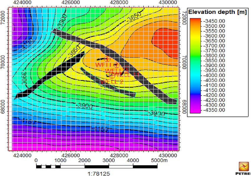
2358 Journal of Petroleum Exploration and Production Technology (2021) 11:2347–2365

Table 7  Average petrophysical Reservoir Vsh ɸt ɸeff K (mD) NTG Sw So h (m) hɸeffSo (m)
properties of analytical results
for reservoir A and B across the A 0.22 0.24 0.19 1185.06 0.78 0.17 0.83 51 8.08
four wells
 B 0.22 0.27 0.21 1360.35 0.78 0.23 0.77 23 3.96

the down thrown blocks are slightly thicker than the correla- reservoir in the Otigwe field by correcting for the present of
tive counterpart of the upthrown blocks. This is attributed shale using net-to-gross ratio, since there is a direct relation-
to successive stages of growth (Childs et al. 2003). This ship between shale volume and net-to-gross. This net-to-
implies that the rock volume or strata in the Niger Delta were gross ratio, porosity and water saturation were then used for
formed contemporaneously and continuously as deposi- the volumetric estimation of the reservoir fluids for proper
tion progresses. According to Lin et al. (2004), such faults estimation of hydrocarbon.
are called syn-depositional extensional faulting, also called The total and effective average porosity determined
growth faults. It was also observed that the faulting is associ- indicate that the reservoir in the Otigwe Field ranges from
ated with anticlinal traps (rollover anticline) across some parts good to very good. The net-to-gross ratio is an engineering
of the seismic sections. The growth fault-rollover anticline correction factor or term use to reduce the volume of the
structural systems result from finite amplitude gravitational unconsolidated sandstone reservoir in the location of study
instability having three different stages of formation, which by correcting the volume of shale.
include; birth, growth and decay (Mauduit and Brun 1998).
The fault-supported anticlinal structural features in the field Time and depth structural maps
were probably responsible for the dispersion and distribution
pattern of sediment and succession of depositional sequences The subsurface time and depth structural maps of the hori-
in the basin. zons of interest (top of reservoir A and B) were constructed
 by posting the time, depth and fault values on the seismic
 base map of the Otigwe Field (Figs. 10, 11, 12, and 13).
Interpretation of petrophysical properties From the depth structural maps, it was observed that the
 contour values where the reservoirs are situated have an anti-
Simulation results of petrophysical properties
 clinal structural trap with network of faults.
Reservoir simulation and modelling software was also used
to estimate the petrophysical properties (Tables 2 and 3). Determination of volumetric estimation
The averages of these modelling results are shown (Table 4).
 The computation of the volumetric estimation in this study
Analytical computation of petrophysical properties was done in both reservoir and surface conditions. Hydro-
from well log carbon reserves or volume of hydrocarbon can be estimated
 using deterministic and stochastic methods. Based on limited
The formulas presented in data set and methods (Eq. 1 to number of available data and geological complexities of the
Eq. 11) were applied for the determination of the various subsurface reservoir, there is always uncertainty in the use of
petrophysical properties (Tables 5 and 6, see computation these methods of estimation. These uncertainties also reflect
in Appendix A). The prolific well for commercial purpose on the volumetric estimation of resource or reserve. There-
was identified to be well 7 from reservoir A, using the factor fore, resources are expected to be estimated by the applica-
hɸeffSo (Table 5). Oil well placement within a grid block of tion of both deterministic and stochastic methods. However,
a reservoir model can be determined by the hɸeffSo factor. in this study, in addition to the approximation made (earlier
The average calculated petrophysical properties are shown discussed), deterministic method was used for the analytical
below (Table 7). method, to determine the volume of hydrocarbon in place,
 The shale volume determination in the preceding section since it is by far the most common. The procedure involves
account for the effect of shale contents within the uncon- the selection of a single value for each reservoir parameter
solidated sandstone reservoir and to ascertain the quality of and input the values into one or more than one simple and
the reservoir within the Otigwe field, coastal swamp depo- appropriate equations, thereby obtaining a single answer.
sitional belt of the Niger Delta. The essentiality of deter- Simple and appropriate equations were used to obtain petro-
mining the shale volume is critical, because it helps in the physical parameters, such as porosity, permeability, water
computation of net-to-gross ratio, porosity and water satura- saturation, net-to-gross ratio, volume of shale, and gross rock
tion (Adeoti et al. 2009). The result of the shale volume was volume. These estimated reservoir parameters and results
used to reduce the volume of the unconsolidated sandstone from seismic interpretation were integrated to obtain a single

 13

Journal of Petroleum Exploration and Production Technology (2021) 11:2347–2365 2359

value for the hydrocarbon pore volume (HCPV) at reservoir Simulated result of volumetric estimation
condition in both reservoirs A and B. This gives a descrip- of reservoir Fluids
tion of the volume of hydrocarbon that filled the pore spaces
inside the reservoir and the change in volume that will take The simulated result of the stock tank oil initially in place
place. This was then converted to volume of hydrocarbon at (STOIIP) (Table 8) indicates that reservoir A is more prolific
surface condition (OOIP or STOIIP) using the appropriate oil compared to reservoir B.
formation volume factor of 1.2 bbl/stb. The estimated volume
of hydrocarbon was calculated directly using average val-
ues of the petrophysical parameters, which include; average Analytical result of volumetric estimation
effective porosity, average oil saturation, average net-to-gross of reservoir fluids
ratio, average of the reservoir thickness in the pay zone and
the reservoir cross-sectional area occupied by oil. The aver- Computation of the area covered with hydrocarbon
age values from these parameters were then substituted into
Eq. (10) to obtain the original oil in place (OOIP) or stock To compute the volume analytically, firstly, the areas of
tank oil initially in place (STOIIP) at surface condition for reservoir A and B were calculated from the depth struc-
both reservoir A and B. tural map (Figs. 10 and 11). The depth structural maps were
 On the other hand, for the simulation model results, divided into squared grids and the area per grid was com-
geostatistical method was used to populate or distribute puted to be 200 m by 200 m (Area = 40,000 ­m3) using the
the reservoir properties, based on Sequential Gaussian survey lines instead of the scale 1:78,125, to avoid printing
Simulation, which considered variogram analysis. The error. The survey lines were traced from the reservoir simu-
procedure or methods was done in such a way that the lation and modelling software and seem accurate. The area
properties at well points where upscaled into the 3D grid in metre was then converted to acre (40,000m3 = 9.88 acres).
and the reason for the upscale is to average the proper- The grids in the maps were counted within the oil region,
ties to feel up the grid cells. After then, the data or vari- taking into consideration the average of the oil water con-
ogram analysis was done to see the variation of the data tacts and the average of the reservoir tops across the four
from one point to another (that is, how far the data could wells. The total oil area for each reservoir was then obtained
remain from point of stationarity or well point to a dis- by multiplying the total number of squared box containing
tance, before it changes to something different). Having oil to the area of a single squared box. Hence, the prospect
understood the data differences, it was now geostatisti- area for each reservoir is as follows:
cally distributed based on neighbour to neighbour cell
changes across the grids (that means that, the cells that • Area of oil region in reservoir A = 9.88 acres × 40 squared
are closed to the well point or point of reference or point grids = 395.20 acres
of stationarity, actually have small features or data simi- • Area of oil region in reservoir B = 9.88 acres × 31 squared
larity and the distribution varies based on the variogram grids = 306.28 acres
distribution or spread). The properties that were distrib-
uted include; the porosity, water saturation, net-to-gross Volumetric estimation of hydrocarbon in reservoir
ratio, permeability, etc. This process is called a stochastic A and B using analytical method
method, because at each point, there is a variation of data
across the grids and not a single property. This was done The volumetric determination approach observes the
for each of the reservoir properties. geological information to estimate the hydrocarbon pore
 Thereafter, model-based calculation was done for each volume and original oil in place. The hydrocarbon pore
of the grid cells to calculate the volume per cell using the volume estimation in this study acknowledged the static
models which comprise each variation of data per cell across method by deriving its source of data from wireline logs
the grids. The basic equation of calculating STOIIP was still and geological base map of the Otigwe field where the
used but the basic difference between the stochastic and the four available logs were located. Thereafter, the forma-
deterministic method is that the deterministic method used tion volume factor was used to convert the hydrocarbon
only a single value (no variation of data—which may really pore volume at reservoir condition to original oil in place
not be realistic due to reservoir heterogeneity resulting from at surface condition (STOIIP). Using the average petro-
facies change) whereas the stochastic method considered the physical properties (Table 7), the computations and results
established variations of STOIIP for each cells across the presentation for reservoir A and B are illustrated below
grids, taking into consideration, the cumulative STOIIP. using Eqs. 9 and 10:

 13

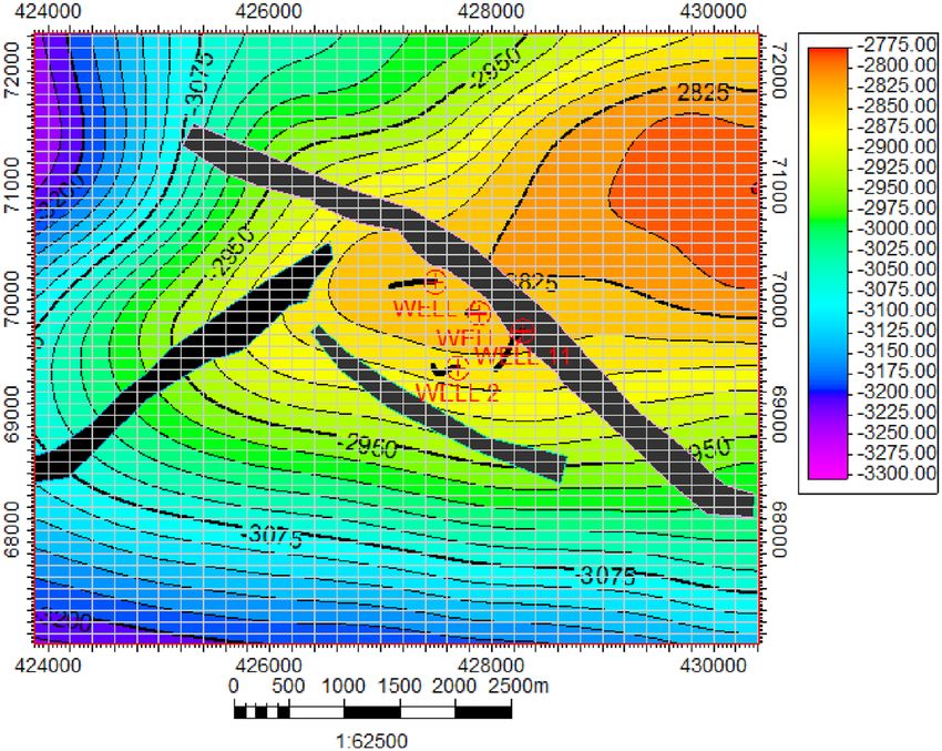
2360 Journal of Petroleum Exploration and Production Technology (2021) 11:2347–2365

Fig. 10  Time structural map of
reservoir A

Fig. 11  Depth structural map of
reservoir A

 13

Journal of Petroleum Exploration and Production Technology (2021) 11:2347–2365 2361

Fig. 12  Time structural map of
reservoir B

Fig. 13  Depth structural map of
reservoir B

 13

2362 Journal of Petroleum Exploration and Production Technology (2021) 11:2347–2365

Volumetric estimation at reservoir condition Table 8  Simulated results of Reservoir STOIIP (MMstb)
 volumetric estimation at surface
Reservoir A: HCPV = 7758 bbl∕acreft × 395.20 acre condition A 59.00
 × 167.32ft × 0.78 × 0.19 × 0.83 B 25.70

 HCPV = 63101671.45 bbl

Reservoir B ∶HCPV = 7758 bbl∕acreft × 306.28 acre more detailed structural architecture and regions of possible
 × 75.46 ft × 0.78 × 0.21 × 0.77 hydrocarbon accumulation within the fault-supported anti-
 HCPV = 22614648.25 bbl clinal trap. This means, faulting and folding were the main
 trapping mechanism in the study area and the four available
 wells were drilled through these traps where most of the
Volumetric estimation at surface condition entrapped hydrocarbons exist.
 The reservoir properties of reservoir A and B in the
Reservoir A Otigwe field indicates that the formation has the potential
 63101671.45 bbl to accumulate reasonable quantity of hydrocarbon, since
STOIIP = = 52.58 × 106 stb = 52.58 MMstb the porosity, permeability, high oil saturation and low water
 1.2bbl∕stb
 saturation values are exceptional, coupled with the right
 Reservoir B entrapment conditions. From the analytical method, the
 identified hydrocarbon-bearing reservoir zones have poros-
 22614648.25 bbl
STOIIP =
 1.2 bbl∕stb
 = 18.85 × 106 stb = 18.85 MMstb ity, permeability and hydrocarbon (oil) saturation ranging
 from 15 to 26%, 893.23 mD to 2323.82 mD and 75% to 92%
 for reservoir A and 18% to 26%, 920.20 mD to 1675.79 mD
Comparing the simulated and analytical STOIIP and 43% to 92% for reservoir B, respectively. Furthermore,
results using the analytical method, the estimated reservoir fluid
 volume (STOIIP) at surface condition for reservoir A is
The simulated result of the stock tank oil initially in place 52.58 MMstb and for reservoir B is 18.85 MMstb, while the
(STOIIP) indicates that reservoir A is more prolific com- average net-to-gross ratio and shale volume for reservoir A
pared to reservoir B. Secondly, comparing the simulated and B are 0.78 and 0.22, respectively. On the other hand,
STOIIP result with that of the STOIIP obtained analyti- from the static model, the identified hydrocarbon-bearing
cally, it was observed that the results for both methods were reservoir zones have porosity, permeability and hydrocar-
closely related (Table 9). bon (oil) saturation ranging from 17 to 24%, 103.10 mD
 to 1783.28 mD and 68% to 79% for reservoir A and 15%
 to 24%, 138.14 mD to 1841.58 mD and 45% to 79% for
Conclusion reservoir B, respectively. Also, the simulation results from
 reservoir simulation and modelling software tool show that
Integrated suites of well logs and 3D seismic data were used the estimated reservoir fluid volume (STOIIP) at surface
to characterise two hydrocarbon-bearing reservoir sand bod- condition for reservoir A is 59MMstb and for reservoir B
ies across four wells in the Otigwe Field, coastal swamp is 25.70MMstb. The average net-to-gross ratio and shale
depobelt, Niger Delta. The reservoir characterisation and volume for reservoir A ranges from 0.86 to 0.89 and 0.11 to
volumetric estimation of the hydrocarbon within the reser- 0.14, respectively, while for reservoir B the range is between
voir sand bodies were made possible through the creation of 0.69 to 0.82 and 0.18 to 0.31, respectively. The estimated
time and depth subsurface structural maps of two horizons reservoir fluid volume using both methods showed similar
of interest using the reservoir simulation and modelling soft- results. The study shows that reservoir A is more prolific
ware. The time and depth subsurface structural maps provide compare to reservoir B.

Table 9  Comparison between Reservoir STOIIP (MMstb) Average OWC (m) Average
Simulated and Analytical reservoir top
Average results of stock tank Analytical result Simulated result (m)
original oil in place (STOIIP)
 A 52.58 59.00 3574 3523
 B 18.85 25.70 2999 2976

 13

Journal of Petroleum Exploration and Production Technology (2021) 11:2347–2365 2363

 From the petrophysical parameters, it can be observed Reservoir A Reservoir B
that the two reservoirs A and B are not uniform due to sub- ( ) ( )
 Vsh = 0.083 23.7×0.5 − 1 = 0.22 Vsh = 0.083 23.7×0.5 − 1 = 0.22
surface reservoir heterogeneity, in addition to the compart-
 Well 9
mentalization with faults and probably fractures which can 60−22.5 60.5−31
complicate fluid flow. Hence, to reduce uncertainty and IGR = 97.5−22.5
 = 0.5 IGR = 90−31
 = 0.5
improve or optimize STOIIP for further studies, it will be
 ( 3.7×0.5
 ) ( 3.7×0.5
 )
 Vsh = 0.083 2 − 1 = 0.22 Vsh = 0.083 2 − 1 = 0.22
ideal to integrate biostratigraphic data and core samples, Well 11
analyse these data and drill more wells around the anticlinal IGR = 62.5−20
 105−20(
 = 0.5 IGR = 81.25−65
 97.5−65
 = 0.5
structure. According to Fadiya et al. (2014), biostratirgaphic 3.7×0.5
 ) ( 3.7×0.5
 )
 Vsh = 0.083 2 − 1 = 0.22 Vsh = 0.083 2 − 1 = 0.22
data play a core role in the integrated characterization and
modelling of lateral continuity of reservoir lithofacies by
providing accurate interpretation of the subsurface reservoir
framework, which aid in decision-making during drilling Analytical computation of total and effective
operation. Hence, with the addition of the biostratigraphic porosity
data and core samples in Otigwe Field, a precise and more
detailed reservoir characterization and volumetric estimation Applying Eqs. (3) and (4) for total and effective porosities,
will be established. respectively, the computation is shown as follows:

 Reservoir A Reservoir B
Implication of the study
 Well 2
From the study, it was discovered that reservoir A and B are Total = 2.65−2.16
 2.65−0.8
 = 0.26 Total = 2.65−2.12
 2.65−0.8
 = 0.29
not homogenous, as can be seen from their variable petro- effective = 0.26(1 − 0.22) = 0.22 effective = 0.29(1 − 0.22) = 0.23
physical parameters (porosity, permeability, etc.), coupled Well 7
with the presence of network of faults around the anticlinal Total = 2.65−2.16
 2.65−0.8
 = 0.26 Total = 2.65−2.1
 2.65−0.8
 = 0.30
structural trap which although indicate that the geometry or effective = 0.26(1 − 0.22) = 0.20 effective = 0.30(1 − 0.22) = 0.23
architecture of the reservoir is good for hydrocarbon accumu- Well 9
lation but these network of faults and probably the presence 2.65−2.3
 Total = 2.65−0.8 = 0.19 Total = 2.65−2.1 = 0.23
 2.65−0.8
of fractures can cause compartmentalization, which can lead effective = 0.19(1 − 0.22) = 0.15 effective = 0.23(1 − 0.22) = 0.18
to complication in fluid flow. Therefore, it will be ideal for Well 11
more wells to be drilled around the fault-supported anticlinal 2.65−2.2
 Total = 2.65−0.8 = 0.24 Total = 2.65−2.16 = 0.26
structural trap, in addition to collecting and analysing core
 2.65−0.8
 effective = 0.24(1 − 0.22) = 0.19 effective = 0.26(1 − 0.22) = 0.20
samples and integrate these core samples with biostratigraphic
data to enhance or optimize the STOIIP in the Otigwe field.

Appendix A Saturation determination

 Applying Eq. (5) and Eq. (6) for water and oil saturation,
 respectively, the computation is shown below with the fol-
 lowing assumptions:
Analytical computation of shale volume
 • The reservoir is water wet
Applying Eq. (1) and Eq. (2) for tertiary or younger rock, the
 • Water salinity is constant
computation is shown as follows:
 • Mud filtrate salinity is constant over the processed inter-
Reservoir A Reservoir B val

Well 2 Based on these assumptions, the resistivity of water for
 52.5−20 53−31
IGR = 85−20(
 = 0.5 IGR = 75−31 (
 = 0.5 each of the oil well, cutting across reservoir A and B, is
 constant.
 3.7×0.5
 ) 3.7×0.5
 )
Vsh = 0.083 2 − 1 = 0.22 Vsh = 0.083 2 − 1 = 0.22
Well 7
 60−20 55−20
IGR = 100−20
 = 0.5 IGR = 90−20
 = 0.5

 13

2364 Journal of Petroleum Exploration and Production Technology (2021) 11:2347–2365

 Reservoir A Reservoir B
 Well 2

In the water zone Sw = 1.0 Rw = 1.02 ×0.202 ×4
 = 0.20 Ωm
 √ 0.81
In the oil zone:
 √
 2 0.81×0.20 2 0.81×0.20
 Sw = 0.202 ×100
 = 0.20 = 20% Sw = 0.232 ×150
 = 0.14 = 14%

 So = 1 − 0.20 = 0.80 = 80% So = 1 − 0.14 = 0.86 = 86%
 Well 7
In the water zone Sw = 1.0 Rw = 1.02 ×0.202 ×3
 = 0.15Ωm
 0.81
In the oil zone:
 √ √
 2 0.81×0.15 2 0.81×0.15
 Sw = 0.202 ×50
 = 0.25 = 25% Sw = 0.232 ×150
 = 0.12 = 12%

 So = 1 − 0.25 = 0.75 = 75% So = 1 − 0.12 = 0.88 = 88%
 Well 9
In the water zone Sw = 1.0 Rw = 1.02 ×0.152 ×3
 = 0.08Ωm
 √ 0.81
In the oil zone:
 √
 2 0.81×0.08 2 0.81×0.08
 Sw = 0.152 ×200
 = 0.12 = 12% Sw = 0.182 ×300
 = 0.08 = 8%

 So = 1 − 0.12 = 0.88 = 88% So = 1 − 0.08 = 0.92 = 92%
 Well 11
In the water zone Sw = 1.0 Rw = 1.02 ×0.192 ×3.5
 = 0.16Ωm
 0.81
In the oil zone:
 √ √
 2 0.81×0.16 2 0.81×0.16
 Sw = 0.192 ×300
 = 0.11 = 11% Sw = 0.202 ×10
 = 0.57 = 57%

 So = 1 − 0.11 = 89% So = 1 − 0.57 = 0.47 = 47%

Analytical computation of net‑to‑gross ratio Reservoir B: K(mD) = 26552(0.23)2 − 34540(0.23)2
 (0.14)2 + 307 = 1675.79 mD.
Applying Eq. (7), the computation is shown as follows: Well 7
 Reservoir A: K(mD) = 26552(0.20)2 − 34540(0.20)2
Reservoir A Reservoir B (0.25)2 + 307 = 1282.73 mD.
Well 2 Reservoir B: K(mD) = 26552(0.23)2 − 34540(0.23)2
NTG = 1 − 0.22 = 0.78 NTG = 1 − 0.22 = 0.78 (0.12)2 + 307 = 1685.29 mD.
Well 7 Well 9
NTG = 1 − 0.22 = 0.78 NTG = 1 − 0.22 = 0.78 Reservoir A: K(mD) = 26552(0.15)2 − 34540(0.15)2
Well 9 (0.12)2 + 307 = 893.23 mD.
NTG = 1 − 0.22 = 0.78 NTG = 1 − 0.22 = 0.78 Reservoir B: K(mD) = 26552(0.18)2 − 34540(0.18)2
Well 11 (0.08)2 + 307 = 1160.12 mD.
NTG = 1 − 0.22 = 0.78 NTG = 1 − 0.22 = 0.78 Well 11
 Reservoir A: K(mD) = 26552(0.19)2 − 34540(0.19)2
 (0.11)2 + 307 = 1250.44 mD.
 Reservoir B: K(mD) = 26552(0.20)2 − 34540(0.20)2
Analytical computation of permeability (0.57)2 + 307 = 920.20 mD.

 Funding The author (s) received no funding for this work.
Applying Eq. (8), the computation is shown as follows:
 Reservoir A: K(mD) = 26552(0.20)2 − 34540(0.20)2 Availability of data This manuscript is an original work conducted by
(0.20)2 + 307 = 1313.82 mD. the authors under close supervision, which restrict data transferability
 Reservoir B: K(mD) = 26552(0.23)2 − 34540(0.23)2 by Moni Pulo (Petroleum Development Limited).
(0.14)2 + 307 = 1675.79 mD.
 Well 2 Declarations
 Reservoir A: K(mD) = 26552(0.20)2 − 34540(0.20)2
(0.20)2 + 307 = 1313.82 mD. Conflict of interest Not applicable.

 Ethics approval Ethics approval has been followed accordingly.

 13

Journal of Petroleum Exploration and Production Technology (2021) 11:2347–2365 2365

Open Access This article is licensed under a Creative Commons Attri- Etu-Efeotor JO (1997) Summarised geology of the Niger Delta. Fun-
bution 4.0 International License, which permits use, sharing, adapta- damental of Petroleum Geology, Jeson Services, Port Harcourt
tion, distribution and reproduction in any medium or format, as long Evamy BD, Haremboure J, Kamerling P, Knaap WA, Molloy FA, Row-
as you give appropriate credit to the original author(s) and the source, lands PH (1978) Hydrocarbon habitat of Tertiary Niger Delta. Am
provide a link to the Creative Commons licence, and indicate if changes Asso Petrol Geol Bull 62:277–298
were made. The images or other third party material in this article are Fadiya SL, Jaiyeola-Ganiyu FA, Fajemila OT (2014) Foraminifera
included in the article’s Creative Commons licence, unless indicated Biostratigraphy and Paleoenvironment of Sediments from Well
otherwise in a credit line to the material. If material is not included in AM-2, Niger Delta. Ife J Sci 16(1):61–72
the article’s Creative Commons licence and your intended use is not Ijasan O, Torres-Verdín C, Preeg WE (2013) Interpretation of porosity
permitted by statutory regulation or exceeds the permitted use, you will and fluid constituents from well logs using an interactive neu-
need to obtain permission directly from the copyright holder. To view a tron-density matrix scale. Interpretation. https://​doi.​org/​10.​1190/​
copy of this licence, visit http://​creat​iveco​mmons.​org/​licen​ses/​by/4.​0/. INT-​2013-​0072.1
 Kulke H (1995) Regional petroleum geology of the world. Part II:
 Africa, Australia and Antarctica. Berlin, Gebruder Bogrntraeger,
 pp 143–172
References Lin C, Zheng H, Ren J, Liu J, Qiu Y (2004) The Control of Syndepo-
 sitional Faulting on the Eogene Sedimentary Basin Fills of the
Abbaszadeh M, Takano O, Yamamto H, Shimamoto T, Yazawa N, San- Dongying and Zhanhua Sags, Bohai Bay Basin. Sci China Ser d
 dria FM, Zamora Guerrero DH, de la Garza, Fernando R (2003) Earth Sci-Eng Ed 47:769–782
 SPE annual technical conference and exhibition, Integrated geo- Mauduit T, Brun JP (1998) Growth fault/rollover systems: birth,
 statistical reservoir characterization of turbidite sandstone depos- growth, and decay. J Geophys Res Solid Earth 103:8B
 its in Chicontepec Basin, Gulf of Mexico. Soc Pet Eng. https://​ Moradi S, Moeini M, Al-Askari MK, Mahvelati EH (2016) Deter-
 doi.​org/​10.​2118/​84052-​MS mination of shale volume and distribution patterns and effective
Adams SJ, Van den Oord RJ (1993) Capillary pressure and saturation porosity from well log data based on cross-plot approach for a
 height functions. Report EP 93–0001, SIPM BV shaly carbonate gas reservoir. IOP Conf Ser Earth and Environ
Adejobi AR, Olayinka AI (1997) Stratigraphy and hydrocarbon poten- sci 44:042002. https://doi.org/10.1088/1755-1315/44/4/042002
 tial of the Opuama channel complex Area, Western Niger Delta. Okolie E, Ujanbi O (2007) Estimation of height of oil-water contact
 Niger Assoc Pet Explor (NAPE) Bull 12:1–10 above free water level using capillary pressure method for effec-
Adeoti L, Ayolabi E, James P (2009) An Integrated approach to volume tive classification of reservoirs in the Niger Delta. Nigerian J Phys
 of shale analysis: Niger Delta example, offrire field. World Appl 9:303–311
 Sci J 7:448–452 Oluwajana OA, Ehinola OA, Okeugo CG, Adegoke O (2017) Modeling
Aizebeokhai A, Olayinka I (2011) Structural and stratigraphic mapping hydrocarbon generation potentials of eocene source rocks in the
 of EMI field, offshore Niger Delta. J Geol Mining Res 3:5–38 agbada formation, Northern Delta Depobelt, Niger Delta Basin,
Ajisafe YC, Ako BD (2013) 3D Seismic attributes for Reservoir Nigeria. J Pet Exp Product Technol 7:379–388
 Characterization of “Y” field Niger Delta Nigeria. J Appl Sci Owolabi O, LongJohn T, Ajienka J (1994) An empirical expression for
 18:86–102 permeability in unconsolidated sands of the eastern Niger Delta.
AL-Awad M, (2001) Evaluating uncertainty in Archie’s water satura- J Pet Geol. https://​doi.​org/​10.​1111/j.​1747-​5457.​1994.​tb001​17.x
 tion equation parameters determination methods. Soc Pet Eng. Passey Q, Creaney S, Kulla J, Moretti F, Stroud J (1990) A practi-
 https://​doi.​org/​10.​2118/​68083-​MS cal model for organic richness from porosity and resistivity logs.
Al-Ruwaili (2007) Accuracy of shaly sand formation evaluation. United AAPG Bull 74:1777–1794. https://​doi.​org/​10.​1306/​0C9B2​5C9-​
 States Patent, Patent no. US 7,168,310 B2 1710-​11D7-​86450​00102​C1865D
Archer JS, Wall CG (1986) Petroleum engineering principles and prac- Short K, Stauble A (1967) Outline of geology of Niger Delta. AAPG
 tice. Grayer and Trotman, London Bull 51:761–779
Archie GE (1942) The electrical resistivity log as an aid in determining Stacher P (1995) Present understanding of the Niger Delta hydrocarbon
 some reservoir characteristics. Trans AIME Soc Pet Eng 146:1–9. habitat. In: Oti MN, Postma G (eds) Geology of Deltas. Rotter-
 https://​doi.​org/​10.​2118/​942054-G dam, AA Balkema
Barde JP, Gralla P, Harwijanto J, Marsky J (2002) Exploration at the Szabo N (2011) Shale volume estimation based on the factor analy-
 eastern edge of the prescapian basin impact of data integration sis of well-logging data. Acta Geophys. https://​doi.​org/​10.​2478/​
 on Upper Permian and Triassic prospectivity. Am Assoc Petrol s11600-​011-​0034-0
 Geol Bull 86:399–415. https://d​ oi.o​ rg/1​ 0.1​ 306/6​ 1EEDA
 ​ EE-1​ 73E-​ Tuttle ML, Charpentier RR, Brownfield ME (1999) The Niger Delta
 11D7-​86450​00102​C1865D petroleum system. Niger Delta province, Nigeria, Cameroon, and
Bridge J, Demicco R (2008) Earth surface processes. Cambridge Uni- Equatorial Guinea, Africa, US Department of the Interior, US
 versity Press, Landforms and Sediment Deposits Geological Survey
Childs C, Nicol A, Walsh JJ, Watterson J (2003) The Growth and Weber MR (2012) A detailed well log and 3D seismic interpretation
 Propagation of Synsedimentary Faults. J Struct Geol 25:633–648 of the fruitland formation: Southwest regional partnership carbon
Dewan JT (1983) Essentials of Modern Open-Hole Log Interpretation. sequestration site, San Juan basin, New Mexico. Master thesis.
 Pennwell Publishing Company, Tulsa, Oklahoma West Virginia University
Doust H (1989) The Niger Delta hydrocarbon potential, a major Ter- Wei Y, Jianbo W, Shuai L, Kun W, Yinan Z (2014) Logging Identifica-
 tiary Niger Province. In: Proceedings of KNGMG symposium, tion of the Longmaxi Mud Shale Reservoir in the Jiaoshiba Area.
 coastal lowstands, Geology and Geotechnology, The Hague. Sichuan Basin Nat Gas Ind B 1(1):230–236. https://​doi.​org/​10.​
 Kluiver Academic Publishers, Dordrecht, pp 22–25 1016/j.​ngib.​2014.​11.​016
Doust H and Omatsola E (1990). Niger Delta. In: Edwards JD, San-
 togrossi PA, (eds) Divergent/passive margin Basins. American Publisher’s Note Springer Nature remains neutral with regard to
 Association of Petroleum Geology Memoir 48: Tulsa, American jurisdictional claims in published maps and institutional affiliations.
 Association of Petroleum Geologists, pp 239–248

 13