Scale-integrated Network Hubs of the White Matter Structural Network
←
→
Page content transcription
If your browser does not render page correctly, please read the page content below
www.nature.com/scientificreports

                         OPEN         Scale-integrated Network Hubs
                                      of the White Matter Structural
                                      Network
Received: 15 December 2016            Hunki Kwon1, Yong-Ho Choi1, Sang Won Seo2 & Jong-Min Lee1
Accepted: 7 April 2017
Published: xx xx xxxx                 The ‘human connectome’ concept has been proposed to significantly increase our understanding of
                                      how functional brain states emerge from their underlying structural substrates. Especially, the network
                                      hub has been considered one of the most important topological properties to interpret a network as
                                      a complex system. However, previous structural brain connectome studies have reported network
                                      hub regions based on various nodal resolutions. We hypothesized that brain network hubs should be
                                      determined considering various nodal scales in a certain range. We tested our hypothesis using the
                                      hub strength determined by the mean of the “hubness” values over a range of nodal scales. Some
                                      regions of the precuneus, superior occipital gyrus, and superior parietal gyrus in a bilaterally symmetric
                                      fashion had a relatively higher level of hub strength than other regions. These regions had a tendency
                                      of increasing contributions to local efficiency than other regions. We proposed a methodological
                                      framework to detect network hubs considering various nodal scales in a certain range. This framework
                                      might provide a benefit in the detection of important brain regions in the network.

                                      The ‘human connectome’ concept, which refers to a comprehensive structural description of the network of ele-
                                      ments and connections forming the human brain, has been proposed to significantly increase our understanding
                                      of how functional brain states emerge from their underlying structural substrates1, 2. While neurons are arranged
                                      in an unknown number of anatomically distinct regions and areas in the human cerebral cortex3, anatomically
                                      distinct brain regions and inter-regional pathways represent perhaps the most feasible organizational level for
                                      the human connectome1, 2. Graph theoretical analysis, a powerful way of quantifying topological properties of a
                                      network, has been adopted in neuroimaging studies to investigate the characteristics of human brain networks
                                      on a macroscale4–8. This makes it possible to consider the human brain as a complex system, where nodes are the
                                      regions of the brain and edges represent the interacting between them. It means that the regions of the human
                                      brain affect each other rather than working independently. For the construction of the structural network of the
                                      human brain, macroscopic gray matter (GM) regions are defined as nodes and the fibers connecting them are
                                      defined as edges in neuroimaging data2, 9–12. Diffusion tensor imaging (DTI), which can measure the structural
                                      integrity of white matter (WM) fiber tracts, is one of the most important imaging modalities for understanding
                                      the structural connectivity between brain regions13, 14. DTI also gives more information on the pathophysiological
                                      procedures than other imaging modalities in terms of brain network analysis4, 8, 15–17.
                                          Many network parameters, which include global network topological properties such as clustering coefficients,
                                      global efficiencies, path length, small-worldness and local network topological properties such as nodal degree,
                                      betweenness centrality, and local efficiencies, have been suggested to explain the topology of the network2, 18.
                                      Especially, the hub, which plays a key role in efficient communication in a network, has been considered one
                                      of the most important topological properties to interpret a network as a complex system19, 20. A network hub is
                                      generally defined as the nodes of network with high degrees or high centrality and is determined based on how
                                      many of the minimum paths between all other node pairs in the network pass through it1. For example, a network
                                      hub of power grids makes it possible to easily distribute the load of one station to other stations, reducing the risk
                                      of serious failure21, 22. A network hub has been considered important in the study of how a disease spreads in a
                                      network because the loss of a hub is likely to break a network into disconnected parts23.
                                          Previous structural brain connectome studies have reported network hub regions based on various nodal
                                      resolutions4, 24–27. Many studies have used a predefined atlas such as the 90 cortical regions from the Automated

                                      1
                                        Department of Biomedical Engineering, Hanyang University, Seoul, South Korea. 2Department of Neurology,
                                      Samsung Medical Center, Sungkyunkwan University School of Medicine, Seoul, South Korea. Correspondence and
                                      requests for materials should be addressed to J.-M.L. (email: ljm@hanyang.ac.kr)

        Scientific Reports | 7: 2449 | DOI:10.1038/s41598-017-02342-7                                                                                     1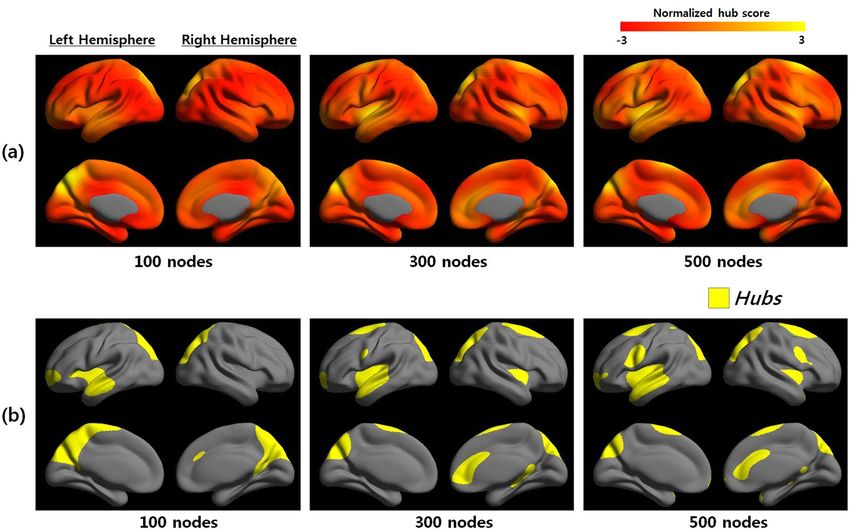
www.nature.com/scientificreports/

                               #Nodal scale           Mean (%)          Std (%)
                               100                    0.1866            0.0237
                               200                    0.0942            0.0156
                               300                    0.0599            0.0114
                               400                    0.0409            0.0079
                               500                    0.0300            0.0063
                               600                    0.0230            0.0052

                              Table 1. The ratio of the number of short fibers and U-fibers to the maximum possible number of connections
                              at each nodal scale. The number of short fibers and U-fibers were determined based on the edges not included
                              in calculation of the network hubs. The ratio showed that the number of short fibers and U-fibers steadily
                              decreased as the nodal scale increased.

                              Anatomical Labeling atlas (AAL)28 to define a network node4, 29. On the contrary, Nijhuis et al. used 500 random
                              regions as nodes to define a network hub30. Hagman et al. used 998 regions that equally cover the whole brain
                              to define the network nodes and show the network hub regions17. Zalesky et al. reported brain network analy-
                              sis results across random subdivisions at scales from 100 to 4000 on the AAL template24. Romero-Garcia et al.
                              also used different cortical sub-regions from 66 to 1494 on the Desikan–Killiany atlas for network analysis26.
                              Supplementary Table S1 summarized the detailed hub regions of these studies. Interestingly, these studies
                              reported different hub regions, which might be due to the strong dependence of network hub regions on the
                              network nodal scale24. The strength of a regional connection was found to positively correlate with the size of the
                              region’s surface in tract-tracing studies of macaque monkeys31. The strength of this relationship between region
                              size and network hub regions might be associated with the number of tracts measured in a given hub region
                              depending on the size of the particular region25. Since most previous studies have defined network hubs after
                              restriction to a specific resolution, they might not capture the potential scale-dependent nature of a node’s role in
                              the network as a whole32. Some studies have shown the strong dependence between hub regions and the network
                              nodal scale, but did not calculate the dependence quantitatively24, 26.
                                  We hypothesized that brain network hubs should be determined considering various nodal scales in a certain
                              range. To the best of our knowledge, the effects of nodal scale on the network hub regions and which regions are
                              scale-integrated hubs (HIS) considering the nodal scale changes have not been examined. We tested our hypoth-
                              esis using the hub strength determined by the mean of the “hubness” values over a range of nodal scales. We
                              normalized the group hub maps of each nodal scale allowing an unbiased comparison between the hub values of
                              multiple nodal scales and defined the HIS on the hub strength map using z-score transformation.

                              Results
                              Ratio of short association fibers. The wiring patterns of WM fibers directly define the topological perfor-
                              mance of brain networks. We computed the ratio of the number of connections of short association fibers (short
                              fibers and U-fibers) to the maximum possible number of connections at each nodal scale to understand how the
                              number of short fibers and U-fibers affect network hubs in different nodal scales (Table 1). The short fibers and
                              U-fibers were defined as the edges but not included in calculation of the network hubs. The ratio showed that the
                              number of short fibers and U-fibers steadily decreased as the number of nodal scales increased.

                              Network hub of multiple scales. Figure 1 showed the average group hub map at each nodal scale.
                              Betweenness centrality maps at different nodal scales were presented, where regions of yellow color indicate
                              higher hub scores than regions of red color (Fig. 1, top). We identified group hubs according to the average
                              betweenness centrality map that were one standard deviation above the mean (see Methods). Hubs of networks
                              at multiple scales were highlighted in yellow (Fig. 1, bottom). The anatomical location of the hubs can be repre-
                              sented from the pre-defined template28 and abbreviations for the cortical regions were listed in Supplementary
                              Table S2. Note that most of the hub regions almost overlapped, among which six cortical regions (precuneus,
                              cuneus, superior temporal gyrus, superior frontal gyrus, superior parietal gyrus, and superior occipital gyrus)
                              appeared as hubs in a bilaterally symmetric fashion between nodal scales. In addition, four brain regions (right
                              middle occipital gyrus, right inferior frontal gyrus, left inferior frontal gyrus, and left Heschl’s gyrus) were con-
                              sidered as hubs only for the coarsest scale; whereas, three different brain regions (right anterior cingulate and
                              paracingulate gyri, left precentral gyrus, and right precentral gyrus) were identified as hubs only in the finest
                              scale. Supplementary Table S3 showed the anatomical locations of the hubs at multiple scales (100–600 scales)
                              and ratio of each hub region compared with pre-defined template.

                              HIS region distribution. The HIS_ST map was shown to demonstrate the overall network hub pattern between
                              multiple nodal scales (Supplementary Figure S1). Figure 2 showed HIS regions with HIS_SC greater than one stand-
                              ard deviation above the mean of the HIS_ST map. Note that, as shown in Table 2, HIS included the regions precu-
                              neus, superior occipital gyrus, superior parietal gyrus, insula, superior temporal gyrus in a bilaterally symmetric
                              fashion, and right cingulum. Additionally, some regions of the precuneus, superior occipital gyrus, and superior
                              parietal gyrus in a bilaterally symmetric fashion had a relatively higher level of HIS_SC than other regions of the
                              insula, superior temporal gyrus in a bilaterally symmetric fashion, and right cingulum.

Scientific Reports | 7: 2449 | DOI:10.1038/s41598-017-02342-7                                                                                    2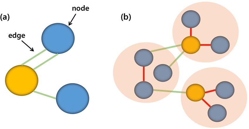
www.nature.com/scientificreports/

                              Figure 1. Betweenness centrality maps and hubs at multiple scales. (a) Betweenness centrality maps were
                              shown at three network nodal scales (100, 300, and 500). The colored scale represented the hub score (red to
                              yellow). (b) Hubs of three network nodal scales were defined by a standard deviation greater than the mean of
                              the betweenness centrality hub map. Supplementary Table S3 showed the network hub at each scale in detail.

                              Figure 2. Distribution of scale-integrated hub (HIS). Z-score transformation was performed to combine the
                              group hub scores from the different scales. Note that the scale-integrated hub score (HIS_SC) captured how ‘well
                              connected’ node i was to other nodes in the scale-integrated hub strength (HIS_ST) map. Regions with a high
                              HIS_SC might also indicate a fundamental hub with high consistency across the nodal scale. Note that Table 2
                              showed the HIS regions in detail.

                              Validation of HIS. We validated whether HIS regions involved a high level of local efficiency by comparing
                              non HIS regions at each nodal scale in order to demonstrate the importance of the HIS regions. The HIS regions
                              had a tendency of increasing contributions to local efficiency than the non HIS regions at most scales (Fig. 3). The
                              p-values, obtained by performing a two-sample t-test for each scale, were also provided to indicate the signifi-
                              cance of difference in HIS and non HIS regions. The local efficiency in HIS regions was significantly higher than
                              that of non HIS regions at 400 nodes (p < 0.05, t-test) or more (p < 0.001, t-test). The Kolmogorov–Smirnov test
                              showed that the distribution of local efficiency in HIS and non HIS regions for each of the nodal scales met assump-
                              tions of normality (p > 0.05).

                              Discussion
                              We proposed a methodological framework to detect network hubs considering various nodal scales in a cer-
                              tain range in this work. Our results suggested that the mechanism for forming structural network hubs is a
                              scale-dependent process and structural network hubs should be determined by investigating the trade-off

Scientific Reports | 7: 2449 | DOI:10.1038/s41598-017-02342-7                                                                                    3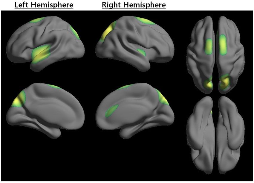
www.nature.com/scientificreports/

                               Anatomical location             HIS_ST     HIS_SC
                               Right superior occipital
                                                               0.980028   4.507347
                               gyrus
                               Left superior occipital gyrus   0.898464   4.095554
                               Right precuneus                 0.948762   4.349493
                               Left precuneus                  0.920223   4.20541
                               Right insula                    0.611848   2.648516
                               Left insula                     0.894113   4.073586
                               Right superior temporal
                                                               0.615138   2.665126
                               gyrus
                               Left superior temporal gyrus    0.961131   4.41194
                               Right superior parietal gyrus   0.980018   4.507295
                               Left superior parietal gyrus    0.878207   3.993282
                               Right cingulum                  0.723567   3.124552

                              Table 2. Scale-integrated hubs (HIS) (scale-integrated hub score (HIS_SC) >1). Anatomical locations of the top
                              11 HIS that had an HIS_SC one standard deviation above the mean.

                              between cortical scales. This framework could provide biologically meaningful results and reduce the bias against
                              network scales by considering all levels of network hubs instead of restricting to one nodal scale. Contrary to
                              previous studies that evaluated network topology at a single nodal network4, 17, 29, 33, our results highlighted the
                              importance of scale integration to detect fundamental brain network topological properties by using HIS_ST. It
                              demonstrated the performance of the suggested method for different numbers of nodes between 100 and 600
                              while avoiding any arbitrary choices.
                                  Some studies have also proposed network hub analysis of multiple nodal scales. Zalesky et al. reported that
                              the cingulate was detected as a region that is highly connected with other regions in the coarsest scale, while the
                              anterior cingulate was detected in only the finest scale24. Romero-Garcia et al. demonstrated that some regions
                              of the middle frontal gyrus, middle occipital gyrus, cuneus, and precuneus were detected in the coarsest scale,
                              while almost all frontal regions, inferior occipital gyrus, inferior parietal gyrus, and precuneus were detected in
                              only the finest scale26. These studies showed that there was a strong dependence between hub region and network
                              nodal scale; however, they did not calculate the dependence quantitatively considering the nodal scale changes.
                                  Some regions of the middle occipital gyrus and inferior frontal gyrus were defined as network hubs at the
                              coarsest scale, but regional heterogeneity was reduced at the finest scale in our results. Other regions of the cin-
                              gulate and precentral gyrus were defined as network hubs in the finest scale. While all of these regions have been
                              reported as network hubs in previous studies9, 29, they were variable according to the nodal scales.
                                  Our findings showed that HIS regions considering all scales were identified in the precuneus, superior occipital
                              gyrus, and superior parietal gyrus regions. The precuneus has mutual corticocortical connections with neigh-
                              boring areas that are responsible for the anatomical basis of their functional coupling and is also connected with
                              other parietal areas related to visuo-spatial information processing34. The precuneus plays a core role in the brain
                              network, suggesting that it has an important function relative to the other regions35. The HIS regions in the precu-
                              neus, superior occipital gyrus, and superior parietal gyrus had a significant negative correlation between age and
                              regional efficiency in a bilaterally symmetric fashion16. Importantly, these HIS regions have also been consistently
                              observed as network hubs9, 29.
                                  It was shown that the HIS regions had significantly greater contributions to local efficiency than the non HIS
                              regions at some nodal scales (400,500 and 600). Note that the HIS regions had a tendency of increasing contribu-
                              tions to local efficiency than the non HIS regions at most scales except for one scale (200). Since network hubs tend
                              to have a high level of local efficiency36, the HIS regions might play an important role in the network and can be
                              considered as fundamental regions, that is, hubs. Although hubs were defined at each scale, our framework can
                              separate them into the HIS regions and the non HIS regions, and the HIS regions had relatively higher betweenness
                              centrality than non HIS regions (Supplementary Figure S2). Our framework method could achieve an increased
                              sensitivity by eliminating the effect of the specific scale on the overall network hub pattern.
                                  We considered that two regions were connected when three fiber tracts were located in these two regions.
                              We analyzed all networks at their fundamental links since structural network based on DTI is naturally sparse.
                              Spurious connections of two regions could be induced by noises or limitations of deterministic tractography. We
                              showed the number of edges according to a threshold of fibers in the Supplementary Figure S3. Even if the thresh-
                              old of fibers was changed, the edges were similar according to nodal scales. It also showed that the important
                              connections having large amount of fibers remained unchanged. We, therefore, selected three fibers as threshold,
                              which was commonly adopted in the previous network studies to eliminate these spurious connections.
                                  The number of short association fibers might affect the varied hub pattern according to the nodal scale. Short
                              association fibers mostly include the local associative fibers (U-fibers) and neighborhood association fibers37.
                              Short association fibers composed of short fibers and U-fibers can have an effect in network hub regions38.
                              Figure 4 showsed an example illustration of how short association fibers can affect hub location according to
                              the nodal scale. Table 1 showed that the number of short association fibers has steadily decreased as the number
                              of nodal scales increased. Previous studies have reported that short association fibers were susceptible to aging
                              effects and were less myelinated, while long association fibers had thicker myelination along the neuron and

Scientific Reports | 7: 2449 | DOI:10.1038/s41598-017-02342-7                                                                                    4
www.nature.com/scientificreports/
Figure 3. Validation of scale-integrated hub (HIS). The HIS regions had a tendency of increasing contributions
to local efficiency than the non HIS regions at most scales. The error bars represented the standard deviation.
Note that ** and * designated statistically significant differences with p < 0.001 and p < 0.05, respectively.
Figure 4. Changes in the network hub position at different scales. A simple graphical model showed a
mathematical description of a network, consisting of nodes (blue circles), hubs (yellow circles), connections
between the nodes (green lines), and u-fibers or short fibers of nodes (red lines). The schematic diagram
represented the different hub regions at different nodal scales.
axon39. It suggested that the removal of short association fibers contributes to lower cognitive efficiency and
higher compensatory brain activation40.
While an HIS_SC of 1 was used to define HIS regions in this study, we validated the various HIS_SC (0.5, 1, 1.5, 2)
values to see their effects on determining the anatomical hub regions (Supplementary Figure S4). The overall hub
distribution showed a similar pattern even if the HIS_SC changed, which might imply that HIS regions have high
consistency of forming a network hub. We also used 1 standard deviation in this study to compare and interpret
with the existing network hub results8, 14–25, 29, 41–52.
We used betweenness centrality to detect network hub regions. Hubs, however, can be detected using other
network centrality measures with high degrees, high closeness centrality, and high rich-club properties compared
with the rest of the network20, 53. Although many studies have used betweenness centrality to examine the regional
hub2, 29, these various measures of centrality could help interpret the meaning of HIS regions in the network. We
used a uniform upsampling of the whole brain surface without respecting anatomical boundaries, which could
take an important role when hub regions are found at the boundaries of the predefined template30.
Romero-Garcia et al. suggested that the best topological trade-off of network scales is in a range from 540–599
and did not differ much from the finest cortical scale26. Nijhuis et al. parcelled neocortical regions into 500 ROIs
to detect network hubs. Many previous studies also investigated anatomical connections by dividing into around
100 regions. Therefore, we used a range from 100–600 nodal scales to determine HIS_SC in this study. Our results
demonstrated that the hub regions that were implied by our proposed methodological framework have important
roles in the study of brain network analysis.
Scientific Reports | 7: 2449 | DOI:10.1038/s41598-017-02342-7 5www.nature.com/scientificreports/
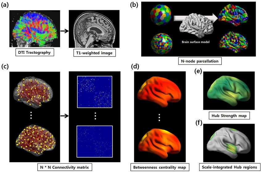
Figure 5. Flowchart of the processing pipeline. (a) The T1-weighted image was rigidly coregistered to the
averaged b0 image in the native diffusion space. The whole-brain WM tracts were reconstructed using the FACT
algorithm. (b) Each neocortical hemisphere was parcellated 20 times into 100, 200, 300, 400, 500, or 600 regions
of interest (ROIs) as nodes using the k-means algorithm determined with the Euclidean distances between
coordinates on the sphere model (left). The parcellated ROIs were transformed to the WM surface matched with
the sphere model (right). (c) Two nodes were considered to be structurally connected by an edge when at least
the end points of three fiber tracts were located in these two regions, and weighted structural networks were
constructed for each individual node at each scale. (d) The betweenness centrality map was calculated 20 times
for each pre-defined individual connectivity matrix dataset using the Brain Connectivity Toolbox (http://www.
brain-connectivity-toolbox.net). Individual betweenness centrality maps were averaged to create the group hub
map. This procedure was repeated for all nodal scales. (e) The scale-integrated hub strength (HIS_ST) is defined
as the sum of all normalized group hub scores divided by the total number of nodal scales in order to estimate
the overall network hub pattern between multiple nodal scales. (f) The scale-integrated hub score (HIS_SC)
captures how ‘well connected’ node i is to other nodes in the HIS_ST map.
Methods
Overview. The aim of the analysis pipeline presented here was to identify network hub regions considering
various nodal scales in a certain range. The flowchart in Fig. 5 described the main steps of our analysis process.
Subjects and MRI acquisition. The Institutional Review Board (IRB) of Samsung Medical Center approved
this study. All participants in this study provided written informed consent. We used a dataset from 54 healthy
subjects from Samsung Medical Center, Seoul, Korea. Three-dimensional (3D) T1 turbo field echo magnetic
resonance (MR) images were acquired using the same 3.0-T magnetic resonance imaging (MRI) scanner (Philips
3.0T 164 Achieva, Eindhoven, the Netherlands) with the following imaging parameters: sagittal slice thickness,
1.0 mm, over contiguous slices with 50% overlap; no gap; repetition time (TR) of 9.9 msec; echo time (TE) of
4.6 msec; flip angle of 8°; and matrix size of 240 × 240 pixels, reconstructed to 480 × 480 over a field of view of
240 mm. The following parameters were used for the 3D fluid-attenuated inversion recovery (FLAIR) images:
axial slice thickness of 2 mm; no gap; TR of 11000 msec; TE of 125 msec; flip angle of 90°; and matrix size of
512 × 512 pixels.
Sets of axial diffusion-weighted single-shot echo-planar images were collected in the whole-brain DT-MRI
examination with the following parameters: 128 × 128 acquisition matrix, 1.72 × 1.72 × 2 mm3 voxels; recon-
structed to 1.72 × 1.72 × 2 mm3; 70 axial slices; 22 × 22 cm2 field of view; TE 60 ms; TR 7696 ms; flip angle 90°;
slice gap 0 mm; and b-factor of 600 smm−2. Diffusion-weighted images were acquired from 45 different direc-
tions with the baseline image without weighting [0, 0, 0]. All axial sections were acquired parallel to the anterior
commissure-posterior commissure line.
Tissue classification and surface modeling. An automated processing-pipeline (CIVET) was used to
extract surfaces of the inner and outer cortex (http://mcin-cnim.ca/neuroimagingtechnologies/civet/)54. Surfaces
consisting of 41,962 vertices were generated for each hemisphere using deformable spherical mesh models after
Scientific Reports | 7: 2449 | DOI:10.1038/s41598-017-02342-7 6www.nature.com/scientificreports/
correction for intensity non-uniformity, normalization to the MNI 152 template, removal of non-brain tissues, and
tissue classification of WM, GM, cerebrospinal fluid, and background using an advanced neural-net classifier54–57.
DTI preprocessing. DTI data was processed using the FMRIB Software Library (http://www.fmrib.ox.ac.uk/fsl).
Motion artifacts and eddy current distortions were corrected by normalizing each diffusion-weighted volume
to the baseline volume (b0) using the affine registration method in the FMRIB’s Linear Image Registration Tool
(FLIRT). Diffusion tensor matrices from the sets of diffusion-weighted images were generated using a general
linear fitting algorithm.
The DTI tractography was performed using the FACT algorithm58 implemented in the Diffusion Toolkit in
the diffusion MR space, and about 100,000 fibers were extracted in each subject (Fig. 5(a)). An angle less than 45°
between each fiber tracking step and minimum/maximum path length of 20/200 mm were included in a thresh-
old set of the terminating condition. The tractography result was masked by the classified WM map.
Parcellating the cortex with different resolutions. Each neocortical hemisphere was parcellated into
100, 200, 300, 400, 500, or 600 regions of interest (ROIs) with similar size as nodes instead of pre-defined anatom-
ical template at single scale. The k-means algorithm was used based on the Euclidean distances between coordi-
nates on a sphere model. The sphere model was made by spherical harmonic parameterization and the nodes were
sampled in a 3D point distribution model (SPHARM-PDM)59. It was repeated 20 times (Fig. 5(b), left) to reduce
the biases for random selection of nodes and size of them for each individual at each nodal scale. Twenty random
nodes were, then, transformed to a WM surface matched with the sphere model (Fig. 5(b), right).
Connectivity matrix and group hub map extraction. T1-weighted images were co-registered to the
b0 images using FLIRT. Reconstructed whole-brain fiber tracts were inversely transformed into the T1 space, and
fiber tracts and surface-based parcellated regions at various scales were located in the same space. Two nodes
were considered to be structurally connected by an edge when at least the end points of three fiber tracts were
located in these two regions, and the edge was defined by the number of fiber tracts. We selected the threshold of
fiber number as three, which was commonly adopted in the previous network studies4, 60–62 to eliminate spurious
connections. Finally, weighted structural networks were constructed for each individual at each scale (Fig. 5(c)).
Nodal betweenness centrality was adopted to examine the regional hub characteristics of the structural brain
networks2, 29. The betweenness centrality (BC) of a node i is defined as
ρjk(i)
BC(i) = ∑ ρjk
j ≠ i≠ k (1)
where ρjk is the number of the shortest paths from node j to node k, and ρjk(i) is the number of the shortest paths
between node j and node k that pass through node i. Hence, BC(i) captures the influence of a node over informa-
tion flow between other nodes in the network. Regions with a high betweenness centrality indicate high intercon-
nectivity with other regions in the network.
The betweenness centrality map was calculated twenty times for each pre-defined individual connectiv-
ity matrix based on random network nodes at each scale using the Brain Connectivity Toolbox (http://www.
brain-connectivity-toolbox.net). The individual betweenness centrality map was taken as an average of the twenty
betweenness centrality maps30. We registered all individual betweenness centrality maps to a group template
using a 2-dimensional surface-based registration algorithm63, 64. They were blurred with a 20 mm full width at half
maximum surface-based diffusion kernel to decrease spatial variability between subjects30. This procedure was
repeated for all nodal scales (Fig. 5(d)).
Identifying HIS regions. Each individual betweenness centrality map was normalized by subtracting the
mean and divided by the standard deviation to allow unbiased comparison between the hub values of all the sub-
jects. Averaged betweenness centrality map (X) at each scale was defined considering all individual betweenness
centrality maps as:
1 N
X(i) = ∑ nBC(k ), (i = 1, 2 … .M )
N k =1 (2)
where nBC(i) is the normalized betweenness centrality map of individual k, N is the sets of all individuals, and
M is the sets of scales. X(i) was calculated by averaging all normalized betweenness centrality maps across all
individuals at each nodal scale. This equation was similar to a previous study65. HIS strength (HIS_ST) was defined
considering all nodal scales as
1 M
HIS _ ST (k ) = ∑ X(i), (k = 1, 2 … .V)
M i= 1 (3)
where X(i) is the averaged betweenness centrality scores of scale i, M is the sets of scales, and V is the sets of ver-
tices. HIS_ST(k) was defined as the sum of all normalized group hub scores divided by the total number of nodal
scales in order to estimate the overall network hub pattern between multiple nodal scales. Note that the uncer-
tainty of hub regions at the multiple nodal scales was averaged out66–68.
The HIS score (HIS_SC) was calculated to detect HIS regions as:
Scientific Reports | 7: 2449 | DOI:10.1038/s41598-017-02342-7 7www.nature.com/scientificreports/
HIS _ ST (i) − µ(HIS _ ST )
HIS _ SC(i) =
σ(HIS _ ST ) (4)
where i is the node index of the HIS_ST map, σ denotes the standard deviation, and µ denotes the mean. Z-score
transformation was performed to combine the group hub scores from the different scales. The HIS_SC could cap-
ture how ‘well connected’ node i is to the other nodes in the HIS_ST map. Regions with high HIS_SC indicated a
fundamental hub with high consistency across nodal scales. While most studies have suggested that z-scores of
betweenness centrality could be used to identify the hub in that community at a single scale38, 41, HIS regions were
defined as regions with HIS_SC greater than a specific standard deviation, which was chosen as 1 in this study, plus
the mean of the HIS_ST map.
Validation analysis. A two-sample t-test was applied at multiple nodal scales to determine the statistical sig-
nificance of the difference in local efficiency between the HIS regions and the non HIS regions at each nodal scale.
The non HIS region was defined as the network hub at each single scale that was not included in the HIS regions.
The network hubs tend to have a high level of local efficiency36. The local efficiency was defined as:
n d −1ij
E (i ) = ∑n − 1
j≠i (5)
where d −1ij is the reciprocal of the shortest paths from node j to node i. We tested whether the HIS regions showed
a higher level of local efficiency than the non HIS regions for each nodal scale. In addition, we used Kolmogorov–
Smirnov normality test to check normality of their distribution using the SPSS Statistics 18 software (http://www.
spss.com/software/statistics/).
Data availability. Patient data was acquired from Samsung Medical Center and may not be made public due
to restrictions from the IRB. Interested researchers may contact Dr. Sang Won Seo, a neurologist at SMC respon-
sible for the data used in this study, to request access to confidential data42–52, 59.
References
1. Sporns, O., Tononi, G. & Kotter, R. The human connectome: A structural description of the human brain. PLoS computational
biology 1, e42, doi:10.1371/journal.pcbi.0010042 (2005).
2. Bullmore, E. & Sporns, O. Complex brain networks: graph theoretical analysis of structural and functional systems. Nature reviews.
Neuroscience 10, 186–198, doi:10.1038/nrn2575 (2009).
3. Van Essen, D. C., Drury, H. A., Joshi, S. & Miller, M. I. Functional and structural mapping of human cerebral cortex: solutions are in
the surfaces. Proceedings of the National Academy of Sciences of the United States of America. 95, 788–795 (1998).
4. Lo, C. Y. et al. Diffusion tensor tractography reveals abnormal topological organization in structural cortical networks in Alzheimer’s
disease. The Journal of neuroscience: the official journal of the Society for Neuroscience. 30, 16876–16885, doi:10.1523/
JNEUROSCI.4136-10.2010 (2010).
5. He, Y., Chen, Z. & Evans, A. Structural insights into aberrant topological patterns of large-scale cortical networks in Alzheimer’s
disease. The Journal of neuroscience: the official journal of the Society for Neuroscience. 28, 4756–4766, doi:10.1523/
JNEUROSCI.0141-08.2008 (2008).
6. Supekar, K., Menon, V., Rubin, D., Musen, M. & Greicius, M. D. Network analysis of intrinsic functional brain connectivity in
Alzheimer’s disease. PLoS computational biology 4, e1000100, doi:10.1371/journal.pcbi.1000100 (2008).
7. Chen, G. et al. Classification of Alzheimer disease, mild cognitive impairment, and normal cognitive status with large-scale network
analysis based on resting-state functional MR imaging. Radiology 259, 213–221, doi:10.1148/radiol.10100734 (2011).
8. Reijmer, Y. D. et al. Disruption of cerebral networks and cognitive impairment in Alzheimer disease. Neurology 80, 1370–1377,
doi:10.1212/WNL.0b013e31828c2ee5 (2013).
9. Stam, C. J. Modern network science of neurological disorders. Nature reviews. Neuroscience 15, 683–695, doi:10.1038/nrn3801
(2014).
10. Fornito, A., Zalesky, A. & Breakspear, M. Graph analysis of the human connectome: promise, progress, and pitfalls. Neuroimage 80,
426–444, doi:10.1016/j.neuroimage.2013.04.087 (2013).
11. Bullmore, E. T. & Bassett, D. S. Brain graphs: graphical models of the human brain connectome. Annual review of clinical psychology
7, 113–140, doi:10.1146/annurev-clinpsy-040510-143934 (2011).
12. He, Y. & Evans, A. Graph theoretical modeling of brain connectivity. Current opinion in neurology 23, 341–350, doi:10.1097/
WCO.0b013e32833aa567 (2010).
13. Basser, P. J., Pajevic, S., Pierpaoli, C., Duda, J. & Aldroubi, A. In vivo fiber tractography using DT-MRI data. Magnetic resonance in
medicine: official journal of the Society of Magnetic Resonance in Medicine/Society of Magnetic Resonance in Medicine. 44, 625–632
(2000).
14. Basser, P. J. & Pierpaoli, C. Microstructural and physiological features of tissues elucidated by quantitative-diffusion-tensor MRI.
Journal of magnetic resonance. Series B 111, 209–219 (1996).
15. Daianu, M. et al. Breakdown of brain connectivity between normal aging and Alzheimer’s disease: a structural k-core network
analysis. Brain connectivity 3, 407–422, doi:10.1089/brain.2012.0137 (2013).
16. Gong, G. et al. Age- and gender-related differences in the cortical anatomical network. The Journal of neuroscience: the official
journal of the Society for Neuroscience. 29, 15684–15693, doi:10.1523/JNEUROSCI.2308-09.2009 (2009).
17. Hagmann, P. et al. Mapping human whole-brain structural networks with diffusion MRI. PloS one 2, e597, doi:10.1371/journal.
pone.0000597 (2007).
18. Rubinov, M. & Sporns, O. Complex network measures of brain connectivity: uses and interpretations. Neuroimage 52, 1059–1069,
doi:10.1016/j.neuroimage.2009.10.003 (2010).
19. Zamora-Lopez, G., Zhou, C. & Kurths, J. Cortical hubs form a module for multisensory integration on top of the hierarchy of
cortical networks. Frontiers in neuroinformatics 4, 1, doi:10.3389/neuro.11.001.2010 (2010).
20. van den Heuvel, M. P. & Sporns, O. Rich-club organization of the human connectome. The Journal of neuroscience: the official journal
of the Society for Neuroscience. 31, 15775–15786, doi:10.1523/JNEUROSCI.3539-11.2011 (2011).
21. Colizza, V., Flammini, A., Serrano, M. A. & Vespignani, A. Detecting rich-club ordering in complex networks. Nature Physics 2,
110–115, doi:10.1038/nphys209 (2006).
Scientific Reports | 7: 2449 | DOI:10.1038/s41598-017-02342-7 8www.nature.com/scientificreports/
22. McAuley, J. J., da Fontoura Costa, L. & Caetano, Tr. S. Rich-club phenomenon across complex network hierarchies. Applied Physics
Letters 91, 084103, doi:10.1063/1.2773951 (2007).
23. Pastor-Satorras, R. & Vespignani, A. Epidemic spreading in scale-free networks. Phys Rev Lett 86, 3200–3203 (2001).
24. Zalesky, A. et al. Whole-brain anatomical networks: does the choice of nodes matter? Neuroimage 50, 970–983, doi:10.1016/j.
neuroimage.2009.12.027 (2010).
25. Bassett, D. S., Brown, J. A., Deshpande, V., Carlson, J. M. & Grafton, S. T. Conserved and variable architecture of human white matter
connectivity. Neuroimage 54, 1262–1279, doi:10.1016/j.neuroimage.2010.09.006 (2011).
26. Romero-Garcia, R., Atienza, M., Clemmensen, L. H. & Cantero, J. L. Effects of network resolution on topological properties of
human neocortex. Neuroimage 59, 3522–3532, doi:10.1016/j.neuroimage.2011.10.086 (2012).
27. de Reus, M. A. & van den Heuvel, M. P. The parcellation-based connectome: limitations and extensions. Neuroimage 80, 397–404,
doi:10.1016/j.neuroimage.2013.03.053 (2013).
28. Tzourio-Mazoyer, N. et al. Automated anatomical labeling of activations in SPM using a macroscopic anatomical parcellation of the
MNI MRI single-subject brain. Neuroimage 15, 273–289, doi:10.1006/nimg.2001.0978 (2002).
29. Gong, G. et al. Mapping anatomical connectivity patterns of human cerebral cortex using in vivo diffusion tensor imaging
tractography. Cerebral cortex 19, 524–536, doi:10.1093/cercor/bhn102 (2009).
30. Nijhuis, E. H., van Cappellen van Walsum, A. M. & Norris, D. G. Topographic hub maps of the human structural neocortical
network. PloS one 8, e65511, doi:10.1371/journal.pone.0065511 (2013).
31. Hilgetag, C. C. & Grant, S. Uniformity, specificity and variability of corticocortical connectivity. Philosophical transactions of the
Royal Society of London. Series B, Biological sciences 355, 7–20, doi:10.1098/rstb.2000.0546 (2000).
32. Ye, A. Q. et al. Measuring embeddedness: Hierarchical scale-dependent information exchange efficiency of the human brain
connectome. Human brain mapping 36, 3653–3665, doi:10.1002/hbm.22869 (2015).
33. Hagmann, P. et al. Mapping the structural core of human cerebral cortex. PLoS biology 6, e159, doi:10.1371/journal.pbio.0060159
(2008).
34. Cavanna, A. E. & Trimble, M. R. The precuneus: a review of its functional anatomy and behavioural correlates. Brain: a journal of
neurology 129, 564–583, doi:10.1093/brain/awl004 (2006).
35. Utevsky, A. V., Smith, D. V. & Huettel, S. A. Precuneus Is a Functional Core of the Default-Mode Network. The Journal of
Neuroscience. 34, 932–940, doi:10.1523/jneurosci.4227-13.2014 (2014).
36. Betzel, R. F. et al. Changes in structural and functional connectivity among resting-state networks across the human lifespan.
Neuroimage 102(Pt 2), 345–357, doi:10.1016/j.neuroimage.2014.07.067 (2014).
37. Yeterian, E. H., Pandya, D. N., Tomaiuolo, F. & Petrides, M. The cortical connectivity of the prefrontal cortex in the monkey brain.
Cortex; a journal devoted to the study of the nervous system and behavior. 48, 58–81, doi:10.1016/j.cortex.2011.03.004 (2012).
38. He, Y., Chen, Z. J. & Evans, A. C. Small-world anatomical networks in the human brain revealed by cortical thickness from MRI.
Cerebral cortex 17, 2407–2419, doi:10.1093/cercor/bhl149 (2007).
39. Catani, M. et al. Short frontal lobe connections of the human brain. Cortex; a journal devoted to the study of the nervous system and
behavior. 48, 273–291, doi:10.1016/j.cortex.2011.12.001 (2012).
40. Gao, J. et al. The relevance of short-range fibers to cognitive efficiency and brain activation in aging and dementia. PloS one 9,
e90307, doi:10.1371/journal.pone.0090307 (2014).
41. Sun, Y. et al. Progressive gender differences of structural brain networks in healthy adults: a longitudinal, diffusion tensor imaging
study. PloS one 10, e0118857, doi:10.1371/journal.pone.0118857 (2015).
42. Tian, L., Wang, J., Yan, C. & He, Y. Hemisphere- and gender-related differences in small-world brain networks: a resting-state
functional MRI study. Neuroimage 54, 191–202, doi:10.1016/j.neuroimage.2010.07.066 (2011).
43. Liao, W. et al. Small-world directed networks in the human brain: multivariate Granger causality analysis of resting-state fMRI.
Neuroimage 54, 2683–2694, doi:10.1016/j.neuroimage.2010.11.007 (2011).
44. Wang, B. et al. Brain anatomical networks in world class gymnasts: a DTI tractography study. Neuroimage 65, 476–487, doi:10.1016/j.
neuroimage.2012.10.007 (2013).
45. Owen, J. P. et al. Test-retest reliability of computational network measurements derived from the structural connectome of the
human brain. Brain connectivity 3, 160–176, doi:10.1089/brain.2012.0121 (2013).
46. Gong, G., He, Y., Chen, Z. J. & Evans, A. C. Convergence and divergence of thickness correlations with diffusion connections across
the human cerebral cortex. Neuroimage 59, 1239–1248, doi:10.1016/j.neuroimage.2011.08.017 (2012).
47. Romero-Garcia, R., Atienza, M. & Cantero, J. L. Predictors of coupling between structural and functional cortical networks in
normal aging. Human brain mapping 35, 2724–2740, doi:10.1002/hbm.22362 (2014).
48. Sporns, O., Honey, C. J. & Kotter, R. Identification and classification of hubs in brain networks. PloS one 2, e1049, doi:10.1371/
journal.pone.0001049 (2007).
49. Li, S. et al. Increased global and local efficiency of human brain anatomical networks detected with FLAIR-DTI compared to non-
FLAIR-DTI. PloS one 8, e71229, doi:10.1371/journal.pone.0071229 (2013).
50. Wu, K. et al. Age-related changes in topological organization of structural brain networks in healthy individuals. Human brain
mapping 33, 552–568, doi:10.1002/hbm.21232 (2012).
51. Kesler, S. R., Gugel, M., Huston-Warren, E. & Watson, C. Atypical Structural Connectome Organization and Cognitive Impairment
in Young Survivors of Acute Lymphoblastic Leukemia. Brain connectivity 6, 273–282, doi:10.1089/brain.2015.0409 (2016).
52. Zhao, Y. et al. Abnormal topological organization of the white matter network in Mandarin speakers with congenital amusia.
Scientific reports 6, 26505, doi:10.1038/srep26505 (2016).
53. van den Heuvel, M. P. & Sporns, O. Network hubs in the human brain. Trends in cognitive sciences 17, 683–696, doi:10.1016/j.
tics.2013.09.012 (2013).
54. Zijdenbos, A. P., Forghani, R. & Evans, A. C. Automatic “pipeline” analysis of 3-D MRI data for clinical trials: application to multiple
sclerosis. IEEE transactions on medical imaging 21, 1280–1291, doi:10.1109/TMI.2002.806283 (2002).
55. Sled, J. G., Zijdenbos, A. P. & Evans, A. C. A nonparametric method for automatic correction of intensity nonuniformity in MRI
data. IEEE transactions on medical imaging 17, 87–97, doi:10.1109/42.668698 (1998).
56. Kim, J. S. et al. Automated 3-D extraction and evaluation of the inner and outer cortical surfaces using a Laplacian map and partial
volume effect classification. Neuroimage 27, 210–221, doi:10.1016/j.neuroimage.2005.03.036 (2005).
57. Collins, D. L., Neelin, P., Peters, T. M. & Evans, A. C. Automatic 3D intersubject registration of MR volumetric data in standardized
Talairach space. Journal of computer assisted tomography 18, 192–205 (1994).
58. Mori, S., Crain, B. J., Chacko, V. P. & van Zijl, P. C. Three-dimensional tracking of axonal projections in the brain by magnetic
resonance imaging. Annals of neurology 45, 265–269 (1999).
59. Styner, M. et al. Framework for the Statistical Shape Analysis of Brain Structures using SPHARM-PDM. The insight journal, 242–250
(2006).
60. Reijmer, Y. D., Freeze, W. M., Leemans, A., Biessels, G. J. & Utrecht Vascular Cognitive Impairment Study, G. The effect of lacunar
infarcts on white matter tract integrity. Stroke; a journal of cerebral circulation 44, 2019–2021, doi:10.1161/STROKEAHA.113.001321
(2013).
61. Shu, N. et al. Diffusion tensor tractography reveals disrupted topological efficiency in white matter structural networks in multiple
sclerosis. Cerebral cortex 21, 2565–2577, doi:10.1093/cercor/bhr039 (2011).
Scientific Reports | 7: 2449 | DOI:10.1038/s41598-017-02342-7 9www.nature.com/scientificreports/
62. Kim, H. J. et al. Clinical effect of white matter network disruption related to amyloid and small vessel disease. Neurology 85, 63–70,
doi:10.1212/WNL.0000000000001705 (2015).
63. Robbins, S., Evans, A. C., Collins, D. L. & Whitesides, S. Tuning and comparing spatial normalization methods. Medical image
analysis 8, 311–323, doi:10.1016/j.media.2004.06.009 (2004).
64. Lyttelton, O., Boucher, M., Robbins, S. & Evans, A. An unbiased iterative group registration template for cortical surface analysis.
Neuroimage 34, 1535–1544, doi:10.1016/j.neuroimage.2006.10.041 (2007).
65. Thompson, W. H. & Fransson, P. The frequency dimension of fMRI dynamic connectivity: Network connectivity, functional hubs
and integration in the resting brain. Neuroimage 121, 227–242, doi:10.1016/j.neuroimage.2015.07.022 (2015).
66. He, Y. et al. Uncovering intrinsic modular organization of spontaneous brain activity in humans. PloS one 4, e5226, doi:10.1371/
journal.pone.0005226 (2009).
67. Achard, S., Salvador, R., Whitcher, B., Suckling, J. & Bullmore, E. A resilient, low-frequency, small-world human brain functional
network with highly connected association cortical hubs. The Journal of neuroscience: the official journal of the Society for
Neuroscience 26, 63–72, doi:10.1523/JNEUROSCI.3874-05.2006 (2006).
68. Ginestet, C. E., Nichols, T. E., Bullmore, E. T. & Simmons, A. Brain network analysis: separating cost from topology using cost-
integration. PloS one 6, e21570, doi:10.1371/journal.pone.0021570 (2011).
Acknowledgements
This research was supported by the Brain Research Program through the National Research Foundation
of Korea (NRF) funded by the Ministry of Science, ICT, & Future Planning (NRF-2014M3C7A1046050);
and by the National Research Foundation of Korea (NRF) grant funded by the Korea government (MSIP)
(2016R1A2B3016609).
Author Contributions
Hunki Kwon and Jong-Min Lee wrote the main manuscript as first author and corresponding author respectively.
Hunki Kwon did network analysis and statistical analysis. Yong-Ho Choi did DTI data processing. Sang Won Seo
acquired the patients’ data as neurologist.
Additional Information
Supplementary information accompanies this paper at doi:10.1038/s41598-017-02342-7
Competing Interests: The authors declare that they have no competing interests.
Publisher's note: Springer Nature remains neutral with regard to jurisdictional claims in published maps and
institutional affiliations.
Open Access This article is licensed under a Creative Commons Attribution 4.0 International
License, which permits use, sharing, adaptation, distribution and reproduction in any medium or
format, as long as you give appropriate credit to the original author(s) and the source, provide a link to the Cre-
ative Commons license, and indicate if changes were made. The images or other third party material in this
article are included in the article’s Creative Commons license, unless indicated otherwise in a credit line to the
material. If material is not included in the article’s Creative Commons license and your intended use is not per-
mitted by statutory regulation or exceeds the permitted use, you will need to obtain permission directly from the
copyright holder. To view a copy of this license, visit http://creativecommons.org/licenses/by/4.0/.
© The Author(s) 2017
Scientific Reports | 7: 2449 | DOI:10.1038/s41598-017-02342-7 10You can also read