Seasonal variability of ocean circulation near the Dotson Ice Shelf, Antarctica
←
→
Page content transcription
If your browser does not render page correctly, please read the page content below
ARTICLE
                  https://doi.org/10.1038/s41467-022-28751-5                 OPEN

                  Seasonal variability of ocean circulation near the
                  Dotson Ice Shelf, Antarctica
                  H. W. Yang1,2, T.-W. Kim 1 ✉, Pierre Dutrieux 3,4, A. K. Wåhlin                                    5,   Adrian Jenkins     6,   H. K. Ha   7,

                  C. S. Kim 8, K.-H. Cho 1, T. Park1, S. H. Lee1 & Y.-K. Cho2
1234567890():,;

                  Recent rapid thinning of West Antarctic ice shelves are believed to be caused by intrusions of
                  warm deep water that induce basal melting and seaward meltwater export. This study uses
                  data from three bottom-mounted mooring arrays to show seasonal variability and local
                  forcing for the currents moving into and out of the Dotson ice shelf cavity. A southward flow
                  of warm, salty water had maximum current velocities along the eastern channel slope, while
                  northward outflows of freshened ice shelf meltwater spread at intermediate depth above the
                  western slope. The inflow correlated with the local ocean surface stress curl. At the western
                  slope, meltwater outflows followed the warm influx along the eastern slope with a
                  ~2–3 month delay. Ocean circulation near Dotson Ice Shelf, affected by sea ice distribution
                  and wind, appears to significantly control the inflow of warm water and subsequent ice shelf
                  melting on seasonal time-scales.

                  1 Korea Polar Research Institute, Incheon 21990, South Korea. 2 School of Earth and Environmental Sciences/Research Institute of Oceanography, Seoul

                  National University, Seoul 08826, South Korea. 3 British Antarctic Survey, Natural Environment Research Council, Cambridge CB3 0ET, UK. 4 Lamont-
                  Doherty Earth Observatory of Columbia University, Palisades, NY 10964, USA. 5 Department of Marine Sciences, University of Gothenburg,
                  Gothenburg, Sweden. 6 Department of Geography and Environmental Sciences, Northumbria University, Newcastle upon Tyne NE1 8QH, UK. 7 Department
                  of Ocean Sciences, Inha University, Incheon 22212, South Korea. 8 National Institute of Fisheries Science, Busan 46083, South Korea.
                  ✉email: twkim@kopri.re.kr

                  NATURE COMMUNICATIONS | (2022)13:1138 | https://doi.org/10.1038/s41467-022-28751-5 | www.nature.com/naturecommunications                          1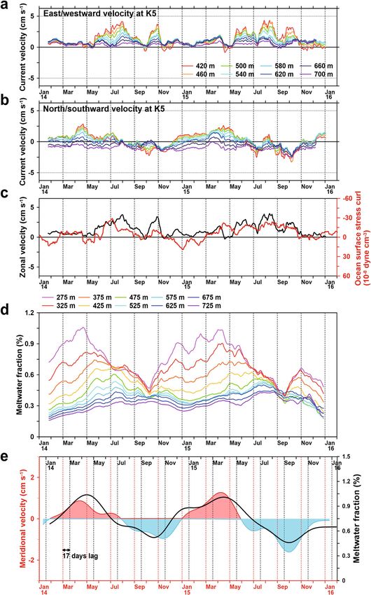
ARTICLE                                                                 NATURE COMMUNICATIONS | https://doi.org/10.1038/s41467-022-28751-5

G
        lacier flow in West Antarctica has been increasing1–5,                the DIS calving front to measure the variability of temperature,
        which can impact global sea-level rise6,7. The cause for the         salinity, and currents. These moorings were located near the
        recent flow increase is believed to be the thinning of the            center of the Dotson–Getz trough (DGT) and on its eastern and
buttressing ice shelves1–3,8. At the Amundsen Sea Embayment                  western slopes, 2–3 km away from the calving front (K4, K3, and
(ASE), ice from the West Antarctic Ice Sheet (WAIS) is drained               K5 in Fig. 1a). The location of the eastern (K4) and western (K5)
into the ocean through the Pine Island, Thwaites, Haynes, Smith,             moorings were chosen to measure mCDW inflows and meltwater
Pope, and Kohler glaciers. These glaciers had an ice flux of                  outflows, respectively. All but one acoustic Doppler current
334 ± 15 Gt yr−1 in 20139, and they have potential to impact sea             profiler (ADCP) recorded successfully for 2 years, while the
level rise globally should this flux change significantly. In the              ADCP measuring near-bottom currents on the eastern mooring
1980s, Pope, Smith, and Kohler Glaciers, located in the western              provided a 1-year record (Supplementary Table 1, Supplementary
ASE, drained ice about 15% of the total ice mass loss from the               Fig. 1).
ASE, but since 2013 their rate have increased and they now
contribute about 23%. In the ASE, warm and salty circumpolar
deep water (CDW) can intrude from the deep ocean across the                  Seasonal variation of mCDW at the eastern and western flank.
continental shelf under the influence of wind and Earth’s                     South-westward currents predominated near the bottom on the
rotation10. This happens in submarine troughs where the seabed               eastern side throughout the record, with an average current speed
is sufficiently deep (>500 m), and in the southern end of these               near 17 cm s−1 at 680 m (Fig. 1a). Away from the seabed, the
troughs a modified version of CDW (slightly colder and fresher                current was somewhat weaker (near 5 cm s−1 at 400 m) and veered
water compared with CDW; mCDW) can access deep-draft ice                     westward. Near the western flank, weak south-eastward flows
which accelerates the ice shelf melt and the glacier mass loss11–17.         (around 1 cm s−1) were measured at 700 m (Fig. 1b). The current
   The oceanic heat transport in the AS is more significant than              direction gradually turned eastward at shallower levels, with an
the Ross and Weddell Seas adjacent to the giant ice shelves in               average current speed reaching 1.2 cm s−1 at 420 m (Fig. 1a).
Antarctica. In the Ross and Weddell Seas, where large cyclonic               Warm and salty mCDW (2 °C higher than the seawater freezing
polar gyres are located north of the continental shelf, only a tiny          point at the surface) was found flowing towards DIS at the eastern
amount of CDW cooled within the gyre intrusion on the con-                   flank below 700 m (Fig. 1c, d), with average temperature and
tinental shelf2,18. Understanding seawater circulation near the ice          salinity for two years at 747 m near the seabed being 0.3 °C and
shelf is essential for determining how changes in oceanic heat               34.5 PSU, respectively. In contrast, the outflows of relatively cold
transport affect basal melting of ice shelves19. Recently, it has            and fresh water (−1 °C, 34.2 PSU) were found above 500 m near
been found that the surface water flowing into the cavity influ-               the western flank (Fig. 1b, e).
ences Ross and Filcher-Ronne ice shelves melting and their                      The predominantly south-westward flow on the eastern flank
seasonality20,21. Long-term mooring observation in front of Pine             (Fig. 2a, b) displayed large, depth-independent seasonal and
Island Glacier (PIG) have shown that the variation in sea surface            intra-seasonal variability. Near the bottom (680 m), the south-
heat flux can affect the variability in CDW volume and seawater               ward (towards the ice shelf cavity) flow reached a maximum of
circulation pattern22. Moreover, the seasonal expansion and                  20 cm s−1 in January 2014 and a minimum of 12 cm s−1 in May.
contraction of polynya and sea ice melting and formation can                 The southward component decreased gradually at mid-depth, but
affect the seawater density structure, affecting the seawater                its seasonal and intra-seasonal variability remained the same in
circulation.                                                                 the whole water column. At the 400 m depth, the observed
   The Dotson Ice Shelf (DIS), located southwest in the ASE,                 maximum southward component was 9 cm s−1 in January 2016,
buttresses the Kohler and Smith Glaciers and has thinned by                  and a northward component of 2 cm s−1 was measured in April
2.6 m yr−1 between 1994 and 2012, which is 30% faster than the               2015. The vertical shear of the meridional current component was
average thickness change in the AS sector (1.94 m yr−1)5.                    largest in the warm layer near the bottom, and it had
Observations near DIS has been conducted semi-regularly in                   comparatively small temporal variations through the measured
summertime since 1994 and demonstrate a substantial inter-                   period. This suggests, that the seasonality of the southward
annual variation connected with the weather systems near the                 component is a barotropic process, and that the baroclinic
ASE15,19. Continuous time series, based on moored instru-                    component (associated with the vertical shear) does not
mentation, are rarer. Although there is a clear seasonal variation           significantly affect the seasonal variability of the southward flow.
of the mCDW intrusions further north in the Getz–Dotson                         In summer, the strong barotropic southward flows drive an
trough10,23, previous records at the ice shelf front15,24,25 have            increase of salinity in front of the DIS (Supplementary Fig. 2)
been too short to determine any seasonality there. The seasonal              because the salinity is relatively low in front of the DIS due to the
variation of atmospheric forcing into the ocean caused by the                strong down-welling26. Salinity at mid-depths (above 500 m)
seasonality of the sea ice distribution will affect the ocean circu-         varied seasonally near the eastern and central front, as shown by
lation near the ice shelf26. Therefore, confirming the seasonality            the 34.2 PSU isohaline, rising from ~450 m in early spring to
of the mCDW circulation in front of the ice shelf and identifying            ~300 m in early summer and deepening 450–500 m for the rest of
the causes is essential for quantifying the influx of oceanic heat            the year. The seawater temperature does not differ significantly
into the ice shelf cavity and understanding the thinning process of          between the eastern slope and the center, similar to the salinity.
the ice shelf. In this study, we show that there is a clear seasonal         Thus, the baroclinic effect by density gradient seems insignificant
variability of mCDW water flowing into the DIS and how it                     in the mid-depth layer. This spatial distribution of salinity suggests
propagates into the cavity beneath the ice shelf. In addition,               that the vertical shear of the southward flow (Fig. 2b) is less
temporal and spatial variations in ocean circulation and heat                prominent in the middle layer (400–560 m) compared to the lower
transport to and from the sub-DIS cavity and look into associated            layer (below 560 m). Nearer the seabed there was no distinct
forcing mechanisms are investigated.                                         seasonal variability of the salinity, but a noticeable eastward
                                                                             gradient increased in association with intrusions of mCDW along
                                                                             the eastern flank. The salinity at 750 m was above 34.5 PSU on the
Results                                                                      eastern side, 34.4 PSU in the center, and 34.35–34.4 PSU on the
Observation. In January 2014, three bottom-moored arrays were                western side. Such a salinity gradient is associated with an increase
deployed from the South Korean icebreaker RVIB Araon along                   of southward current shear near the bottom.

2                NATURE COMMUNICATIONS | (2022)13:1138 | https://doi.org/10.1038/s41467-022-28751-5 | www.nature.com/naturecommunications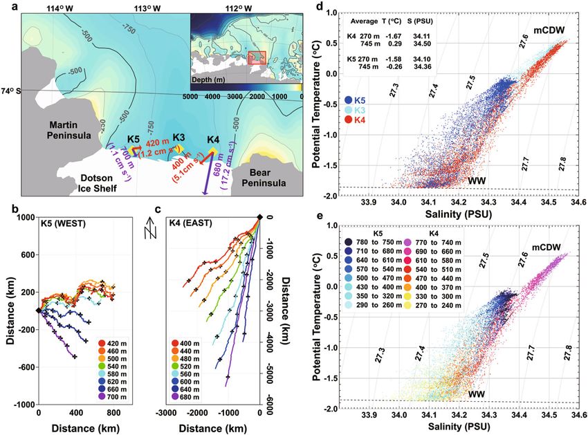
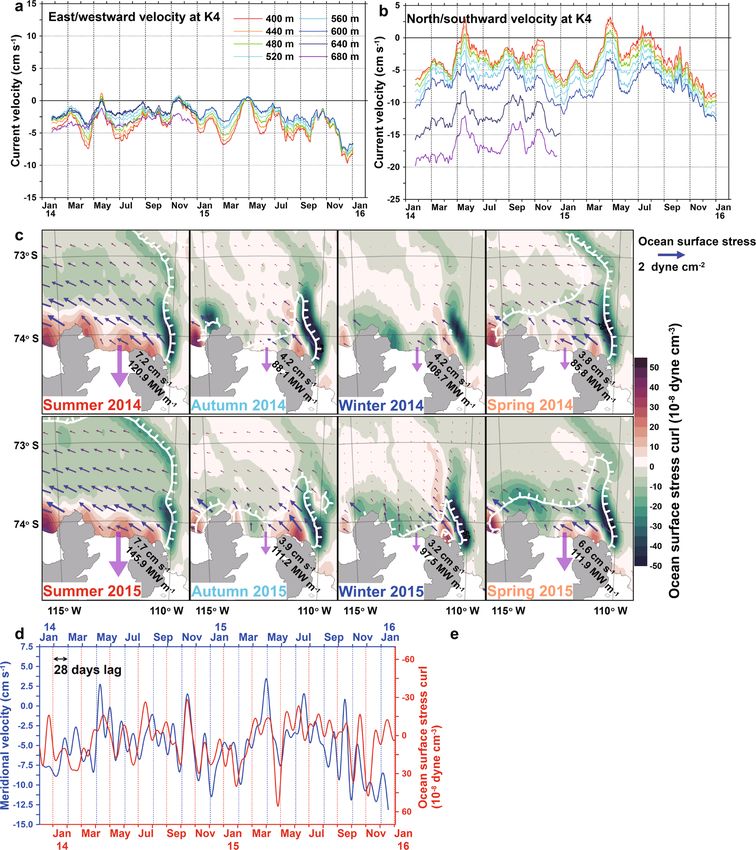
NATURE COMMUNICATIONS | https://doi.org/10.1038/s41467-022-28751-5                                                                      ARTICLE

Fig. 1 Study area, bathymetry, station locations, progressive vector and temperature–salinity diagrams at mooring sites. a Bathymetry, coastline66, and
stations on the Amundsen Sea continental shelf (location shown in red rectangle). Yellow diamonds show moorings K3–K5 near the Dotson Ice Shelf. Red
and purple arrows are average current at the top layer (K4 = 400 m, K5 = 420 m) and the bottom layer (K4 = 680 m, K5 = 700 m). b, c Progressive
vector diagrams of velocities at K5 from 420–700 m depth and K4 from 400–680 m depth during 2014 and 2015. Color-coded dots denoted depth and
marked the black cross on the diagrams every 3 months interval. Black diamonds are the starting point. d Temperature–salinity at K4 (red), K3 (cyan), and
K5 (blue). Average potential temperature and salinity near the top (270 m) and bottom layer (745 m) are highlighted. e Temperature–salinity color-coded
by the depth at K4 and K5.

Effect of ocean surface forcing. North of the DIS, the Amundsen                 Therefore, although both buoyancy flux and meridional velocity are
Sea polynya (ASP) repeats seasonal expansion and contraction,                   influenced by atmospheric variability and vary seasonally, the effect
which can affect seawater circulation and spatial distribution of               of local buoyancy fluxes on mCDW variability and circulation are
mCDW by causing changes in ocean surface density during sea                     comparatively weak in the present data set.
ice formation and melting. Previous study from PIG22 suggests                      At the outer edges of the ASP, there is a boundary between
that local positive (i.e., from ocean to air) buoyancy fluxes from               open water and (more or less) fast sea ice. When a homogeneous
sea ice formation and/or atmospheric cooling (less buoyant at the               wind field blows over an opening in the fast ice, spatial stress
sea surface) creates deep convection, leading to a downward                     gradients (ocean surface stress curl, OSSC, Fig. 2c) are created
descent of the thermocline and thinning of the mCDW layer at                    near the edges, resulting in divergence or convergence of the
the bottom, while negative buoyancy fluxes (i.e., downward and                   wind-driven surface (Ekman) transport23. These can induce
more buoyant at the sea surface) due to surface heating and sea                 barotropic currents. In other to estimate the effect of the
ice melting leads to an upward movement of the thermocline and                  barotropic component on the variability of the southward current
a increase mCDW volume. In order to investigate the effect of sea               near the eastern side of DIS front, the OSSC was calculated from
ice fluctuations on the change of mCDW and its circulation, local                sea ice motion and wind using the ice–ocean drag coefficient (see
surface buoyancy fluxes were calculated using the heat- and                      the “Methods” section and Supplementary Fig. 4) and compared
freshwater fluxes from the data-assimilating Southern Ocean                      to the mooring data. The variability of OSSC on the eastern flank
State Estimate (SOSE)27. These surface buoyancy fluxes were then                 was relatively high compared to the western flank. Cross-spectral
compared to the depth of isohalines and meridional velocities                   analysis of the OSSC at the eastern flank (74°S, 112.25°W) and the
(Supplementary Fig. 3a and see the section “Methods”). Both                     vertically averaged southward velocity at mooring K4 showed a
local buoyancy flux and meridional velocity demonstrate a sea-                   statistically significant coherence around 80-day frequency with
sonal variation that decreased in summer and increased in winter.               other shorter frequencies (e.g., 31-day and 22-day) (Supplemen-
The buoyancy flux, which affects the density structure of the                    tary Fig. 5). In addition, 20-day low-pass-filtered southward
water column, modulates the baroclinic component of the mer-                    velocity had a statistically significant correlation (r = 0.47) with
idional velocity. However, the variation range of the baroclinic                OSSC at 28-day lag (Fig. 2d, e), approximately a quarter of a
component (depth-averaged removed) in meridional velocity was                   combines of a dominant 80-day frequency and other shorter
5.67 cm s−1 at 680 m depth, which was the largest in the entire                 frequencies, suggesting that the accumulated OSSC forces variation
layer, but almost half of the barotropic component of 11.52 cm s−1.             in the barotropic meridional velocity. That is, positive OSSC along

NATURE COMMUNICATIONS | (2022)13:1138 | https://doi.org/10.1038/s41467-022-28751-5 | www.nature.com/naturecommunications                               3
ARTICLE                                                                   NATURE COMMUNICATIONS | https://doi.org/10.1038/s41467-022-28751-5

                                                                                                                0.2

                                                                                                                0.1
                                                                                            Cross Correlation

                                                                                                                  0

                                                                                                                -0.1

                                                                                                                -0.2

                                                                                                                -0.3

                                                                                                                -0.4
                                                                                                                              Lag (day)
                                                                                                                -0.5
                                                                                                                  -60   -40   -20      0        20   40   60
                                                                                                                                    Lag (day)

Fig. 2 Time series of velocities and ocean surface stress curl. a, b 31-day running average zonal and meridional velocities at K4 (East flank). Positive
values indicate east and northward currents. c Horizontal distribution of ocean surface stress curl (color), ocean surface stress (arrow) and sea ice
concentration (SIC) in 2014 and 2015. Outside of the white line indicates where SIC is over 50%. A positive ocean surface stress curl (OSSC) means high
sea surface height. The seasonal average southward velocity and heat transport are shown on the map, and the purple arrows indicate the magnitude of
southward heat transport. d 20-day low-pass filtered OSSC at 74°S, 112.25°W (red) and vertical mean (400–600 m) meridional velocity (blue). Axis of the
OSSC was reversed. e Cross-correlation between OSSC and velocity with 20-day low-pass filter and 99% confidence interval (blue line).

the eastern slope of the DIS increases the cumulative OSSC,                    flank creates a zonal barotropic pressure gradient driving a
increasing the horizontal gradient of the sea surface elevation and            southward velocity. During summer, the OSSC increases due to
accelerating the barotropic southward flow. When the positive                   strong south-easterly winds over the open sea and during winter it
OSSC turns negative, the barotropic southward flow is maximum                   decreases when the wind stress and currents are weakened by the
and then decelerates. We interpret this statistically significant               sea ice cover (Fig. 2c). The summertime increase of the OSSC leads
relationship as an indication that higher OSSC over the eastern                to a strengthened southward mCDW flow (Supplementary Fig. 6a)

4                  NATURE COMMUNICATIONS | (2022)13:1138 | https://doi.org/10.1038/s41467-022-28751-5 | www.nature.com/naturecommunications
NATURE COMMUNICATIONS | https://doi.org/10.1038/s41467-022-28751-5 ARTICLE
and enhanced heat transport to the ice shelf. Conversely, both gradient increasing to the east causes an increase in the
southward flow and heat transport decrease in winter. The southward baroclinic current countervailing the northward
relatively high OSSC near the DIS can also induce a barotropic barotropic current.
pressure gradient in the meridional direction, which may similarly During summer and autumn, the input of glacier meltwater in
drive the strongly barotropic westward Antarctic coastal current at the Dotson trough strengthens athe stratification and prevents
mid-depth (Fig. 2a). The westward current component decreases vertical convection of dense water31. However, the decrease of
with depth due to the eastward baroclinic shear caused by the local meltwater discharge in the winter and spring would weaken the
down-welling associated with high OSSC near the ice shelf front. stratification and enhances the deep convection of dense winter
On the western flank of the ice shelf front, the seasonal water. An upper water column homogenized by vertical mixing
variation, most prominent in mid-depth, had a range about half can provide an opportunity for the winter water to descend to the
that of the eastern side bottom (Fig. 3a, b). Near the bottom, near- middle layer. This strengthening of vertical convection and the
constant weak south-eastward currents were observed during the Antarctic Coastal Current26,29 to the westward can rapidly reduce
entire record. The meridional current component shifted between the upper layer meltwater fraction (Fig. 3d).
northward in fall and southward in spring (Fig. 3b) and the
current velocities were generally smaller compared to the eastern
Relation between heat transport and meltwater flux. In order to
flank. In both 2014 and 2015, the highest northward velocities
evaluate the effect of warm water inflow and its seasonality on the
were 2.9 and 2.5 cm s−1 in April and the highest southward
basal melting, heat transport toward the DIS near its eastern front
velocity was 2.5 cm s−1 in early October. The eastward current
was estimated as a function of heat content and southward cur-
component had a maximum in winter, 4.2 and 4.9 cm s−1 at
rent velocity for the two years (see the “Methods” section and
420 m depth in July (Fig. 3a), and was almost constant close to
Fig. 4). The heat transport varied between 51 and 182 MW m−1,
2 cm s−1 in summer. The occurrence of eastern flow in the winter
with summertime values more than three-fold those of winter due
coincides with a decrease of OSSC at the western side of DIS front
to the strengthened southward velocities and higher seawater
(Fig. 3c), and an associated local drop in sea level height,
temperature near the bottom. Although the peak of heat transport
intensifying the eastward barotropic current in the entire water
in winter was smaller than that in summer, it was conspicuous
column. However, the upwelling accompanied by negative OSSC
(July 2014 and June 2015, Fig. 4b) compared to the small peaks in
generates a westward baroclinic current that countervails the
spring and autumn. Such two winter peaks mainly depend on the
eastward barotropic current at a deeper in the water column.
strengthening of the southward flow and are related to the
increase of OSSC due to the strengthening of the wind (Supple-
mentary Fig. 9).
Meltwater outflow. During all seasons, there was a weak south-
Although it is expected that the seasonal increase in heat
ward flow present near the bottom throughout the record at the
transport has implications for the basal melt of the ice shelf, recent
western side of DIS front (Fig. 3b), presumably driven by the
results indicate that the barotropic current component, which is a
cross-front salinity distribution which increased toward the
strong contributor to the seasonal variability, can be at least partially
eastern side of DIS due to the inflow of mCDW. In the middle
blocked at the ice front32. Nevertheless, the seasonal variability of
layer, the northward current component had a seasonal max-
heat transport in front of the ice shelf will be propagated to under
imum in autumn, both years, coinciding with maximums of the
the ice shelf because the barotropic southward flows affect the
meltwater fraction (e.g. concentration of glacial meltwater in
variability of isohalines and isotherms, and that signal is expected to
seawater calculated by Eqs. (3) and (4) in the “Methods” section)
propagate in the cavity (Supplementary Fig. 3). The oceanic heat
(Fig. 3b, d). These meltwater outflows occurred mainly in the
transport along the eastern slope melts the DIS base, and a fresh
layer between 272–540 m and can be significant enough to
meltwater mixture returns to the open sea along the western slope.
influence the density structure in the water column and thereby
Meltwater fluxes on the west side seemingly follow heat transports
the local circulation26,28. Since the mooring did not cover the
on the east side with a 74-day lag (correlation of r = 0.50 on a 99%
upper water column, it is believed that much of the meltwater
significance level, Fig. 4b, and Supplementary Fig. 10). Such a
outflow remained undetected (Supplementary Fig. 7). However,
significant correlation indicated that the heat transport to the ice
the signal is sufficiently strong to identify the seasonal variation of
cavity affected by the OSSC variability at the eastern slope causes
the outflow. We observe a seasonal variation of the meltwater
the seasonal variation of meltwater discharge and northward flow at
fraction (Fig. 3d, see the “Methods” section), with a maximum
the western slope. The observed delay between warm inflow and
exceeding 1% in April for 275 m depth in both years. This value is
meltwater outflow agrees qualitatively well with the two months
similar to PIG (~1.5% at 100–500 m)29 and Shirase Glacier
residence time inside the cavity observed in 201833. Our new
Tongue in East Antarctica (near 0.8%)30. The seasonal phase of
observation on the variability of seawater circulation in front of ice
the maximum meltwater fraction is delayed gradually toward the
shelves and the link between heat inflow to the ice cavity and
bottom, with the maximum at 575 m (0.45%) appearing in July.
meltwater discharge complements the previously revealed mechan-
In contrast, the minimum meltwater fraction appeared in early
ism by Jenkins et al. (2018)34 that heat content variability in front of
October/September both years for the whole water column.
DIS can affect the heat transport into the DIS cavity and ice
A decrease of vertically integrated density along the western
shelf melt.
side of the ice front by a discharge of meltwater during autumn
leads to local sea surface elevation rise and an increase in the
northward barotropic current. There is a strong correlation Discussion
(r = 0.9, with a 17-day lag) between the meridional current Using two years of mooring data near the calving front of Dotson
velocity and the upper layer meltwater fraction (Fig. 3e and ice shelf, we identified a substantial inflow of warm and salty
Supplementary Fig. 8). Thus, the variability of meridional current water near the seabed at the eastern flank of the deep trough that
at the western side of DIS may be influenced by meltwater leads into the ice shelf cavity. We also identified high con-
discharge. This is in contrast to the eastern side, where it is centrations of meltwater on the opposite (western) flank. These
primarily OSSC that changes the velocity. Deeper in the water findings have been observed in other systems that receive warm
column, the freshening by an inflow of meltwater in the water salty water through deep troughs in the continental shelf, such as
column reduces the density in the western front. The density Getz ice shelf32,35, Pine Island Glacier19, Amery ice shelf36, as well
NATURE COMMUNICATIONS | (2022)13:1138 | https://doi.org/10.1038/s41467-022-28751-5 | www.nature.com/naturecommunications 5ARTICLE NATURE COMMUNICATIONS | https://doi.org/10.1038/s41467-022-28751-5 Fig. 3 Time series of velocities and meltwater fraction at K5. a and b 31-day running average zonal and meridional velocities at K5 (West flank). c 31-day running average zonal velocity (420 m, black line) and mean ocean surface stress curl (OSSC) (74°S, 112.75–113.25°W, red line). r = 0.57, confidence level = 99%. d 31-day running average meltwater fraction at 50 m intervals from 275 to 725 m (thin color-coded lines). e Velocity (vertical mean) and meltwater fraction (black line) at 275 m with 90-day low-pass filter (r = 0.9, with a 17-day lag). Red and blue shades indicate northward and southward flow, respectively. The upper x-axis is back-shifted by 17-day. as Dotson trough further north than the presently studied Both the warm inflow in the east and the meltwater outflow in system37. A similar circulation pattern has also been noted in the west had a clear seasonal variation. Inflow velocity and heat comparatively ‘cold’ shelf systems such as Ross ice shelf20 and content in the east peaked in summer, with a nearly three-fold Filchner-Ronne ice shelf38, although it does not substantially increase of the summertime heat transport toward the cavity. influence the ice shelf melt processes there. It was also shown that There was also an autumn maximum in both meltwater content high meltwater concentrations correlate with intermittent out- and outflow velocity in the western side of the ice shelf front, flows from the western side of the cavity, which is to be expected delayed by about 2 months from the inflow peak in the east. The but is rarely observed due to the challenging environments for substantial seasonal variability of heat transport and meltwater data collection near the calving fronts of these large glaciers. discharge near the ice shelf calving front, that was observed, 6 NATURE COMMUNICATIONS | (2022)13:1138 | https://doi.org/10.1038/s41467-022-28751-5 | www.nature.com/naturecommunications
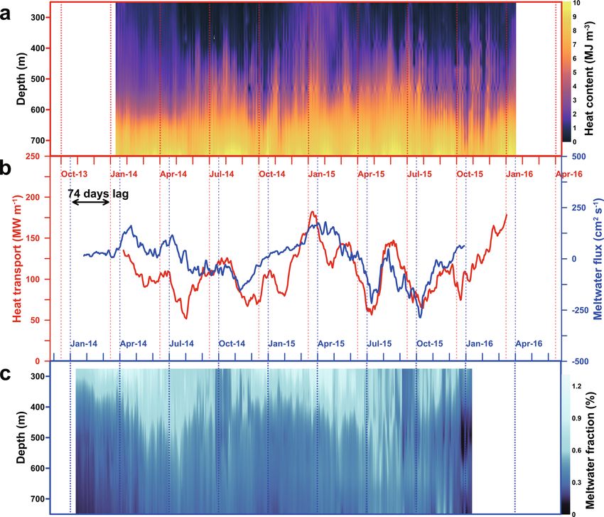
NATURE COMMUNICATIONS | https://doi.org/10.1038/s41467-022-28751-5                                                                    ARTICLE

Fig. 4 Time series of heat content and heat transport at K4 and meltwater fraction and meltwater flux at K5. a Vertical and temporal distribution of
calculated heat content from 250 to 750 m at K4. b 31-day running average vertical mean meltwater flux(blue) between 275 and 575 m at mooring K5 and
estimated heat transport (red) at mooring K4. The upper x-axis for heat transport and content has been back-shifted 74-day. c Vertical and temporal
distribution of meltwater fraction at mooring K5.

suggests that previously evaluated heat- and meltwater                          and sea ice conditions. These appear to be similar to the inter-
transport15,24,25, based on summer observation, may have been                   mittent reductions in heat transport that have been observed at
overestimated. Based on the present data set the average heat                   the Getz ice shelf cavity35, except that the forcing in the present
transport in summer was 141 MW m−1, 1.27 times greater than                     locality is mainly local while the Getz ice shelf appears to be
the annual average of 111 MW m−1, a number that can be used to                  predominantly remotely forced and transmitted via topographic
scale summertime observations from this region. The seasonal                    waves to the cavity opening.
average meltwater flux to the north was at a maximum of                             The driving mechanism behind seasonality of the heat trans-
89.2 cm2 s−1 in autumn and 25.7 cm2 s−1 in summer. In contrast,                 port into the DIS cavity is interpreted to be caused by local OSSC,
meltwater flux showed negative in winter and spring due to the                   induced by changes in sea ice and wind distribution, in turn
dominant southward flows, and the annual average was close to                    linked to changes of the polynya area and sea ice distribution40.
zero. This seasonality implies that additional observations are                 Previous studies have shown that the wind field and atmospheric
needed to determine how much of the inter-annual variability of                 circulation affects not only the seawater circulation at the ice shelf
heat and meltwater transport seasonality propagates into the ice                front but also the variability of warm water flowing into the DGT
shelf cavity. The effects of the strong seasonality also have                   near the center of the continental shelf10,11,23,41. Also, local wind
implications for timing of snapshots used to calculate ice shelf                forcing in front of PIG has been attributed a significant mod-
thickness evolution and points to the importance of high-                       ulator for the short-term (less than one month) variability of the
resolution remote sensing products when calculating ice shelf                   upper thermocline depth and basal melting there42. Local atmo-
mass balance.                                                                   spheric forcing, such as wind, is the most crucial factor in
   The seasonal variation observed at DIS is in contrast to sea-                determining the variability of the seawater circulation and oceanic
sonal variation in the deep troughs leading to Pine Island                      heat transport in the AS. Meanwhile, atmospheric circulation in
Glacier22 and to Getz Glacier32,35,39, where a wintertime max-                  the AS is much more complex and diverse than in any other sea
imum in heat content and velocity has been observed. In contrast                in Antarctica due to the variability43,44 (i.e., seasonal migration of
to the situation at Pine Island Glacier calving front22, where the              longitudinal location) in the Amundsen Sea Low (ASL)45. In
main cause for vertical migration of the thermocline is local                   addition, this variability in ASL was influenced by the Southern
buoyancy flux, short-term variability of heat transport was here                 Annular Mode (SAM) and El Niño-Southern Oscillation (ENSO)
caused by local changing stress at the ocean surface due to wind                phases in a long-term timescale46.

NATURE COMMUNICATIONS | (2022)13:1138 | https://doi.org/10.1038/s41467-022-28751-5 | www.nature.com/naturecommunications                            7
ARTICLE NATURE COMMUNICATIONS | https://doi.org/10.1038/s41467-022-28751-5
Through long-term observations in front of DIS for two years,
we found that heat was delivered to the DIS cavity along the T;S χ T χTCDW
ψ melt ¼ χ Tmelt χ TCDW χ Smelt χ SCDW χ WW
eastern flank of the DGT, and glacial meltwater was emitted along WW χ CDW
S S
T S χTWW χTCDW
the western flank with a time lag of two months. Furthermore, the T;S
ψ mix ¼ χ obs χ CDW χ obs χ CDW χS χS
T S
ð4Þ
WW CDW
seasonality of heat transport and meltwater discharge was con- ψ T;S
firmed due to the variability of OSSC induced by wind and sea ice φ¼ mix
ψ T;S
melt
distribution. The circulation pattern of mCDW in the front of the where χT and χS represent potential temperature and salinity and subscripts melt,
ice shelf and its seasonal variability by atmospheric conditions CDW, WW, and obs indicate the end-members of ice, CDW, Winter water, and
demonstrated here allow for quantitative evaluation of the effects in situ observations at K5. In previous studies, meltwater fraction calculation and
of short-term variability in the atmosphere on ocean circulation. end-member selection have used summer observation data24,34,48–50. In this study,
an end-member applicable over the entire season was required to calculate the
This finding implies that the ocean circulation effect by local meltwater fraction using mooring data. However, winter water is generated as a
meteorological conditions in front of the ice shelf plays an result of brine rejection and convection by sea surface cooling and remains until
essential role in regulating mCDW inflow and the basal melting summer above the mCDW layer. Thus, to detect this ‘pure’ winter water, we
of the ice shelf. Therefore, understanding the long-term varia- selected end-member estimated from summer observation already presented. We
bility of the atmosphere and the subsequent response of the ocean used the two-year average (2014 and 2016) end member for CDW (T ~ 0.013 °C,
S ~ 34.46 PSU), WW (T ~ −1.88 °C, S ~ 34.24 PSU) and ice (T ~ −95 °C, S ~ 0 PSU)
circulation are likely essential for determining the long-term obtained from previous studies in the AS34.
melting trend of the WAIS. These results suggest that further
studies are needed, e.g., ice-ocean coupled numerical model study Buoyancy flux calculation. Buoyancy flux is caused by atmospheric heating and
considering the ice shelf. formation and melting of sea ice. Buoyancy flux was calculated as
QHF
Methods Bf ¼ gα þ gβQFW S0 ð5Þ
ρw C p
Data collection. To monitor the temporal and spatial variation of mCDW and its
effect on the rapid melting of glaciers in the Amundsen Shelf, we conducted where g is acceleration of gravity (9.8 m s−2) and α at the sea surface (35 PSU, 0 °C)
extensive oceanographic surveys 4 times from 2010 to 2016. The temporal varia- is the thermal expansion coefficient (5.1 × 10⁻⁵ K−1)51. QHF is net air–sea heat flux
bility and properties of mCDW and its circulation in front of the DIS were (W m−2) and positive means that the ocean gains heat. ρw and Cp are water density
obtained from the K3–K5 moorings deployed on January 8–9 2014, and recovered and specific heat of seawater (4190 J kg−1 K−1), respectively. β (at the sea surface,
on January 19–20, 2016. At each station, the current velocities were observed from 35 PSU, 0 °C) is the saline contraction coefficient (7.9 × 10⁻⁴)51. QFW is the
dual ADCPs with upward-looking 150 kHz (K4 and K5) or 75 kHz (K3) and freshwater flux (m s−1) and negative means that the ocean gains fresh water. S0 is
downward-looking 300 kHz (K3–K5) RD Instruments (RDI) (Supplementary the ocean surface salinity. QHF and QFW are obtained from the data-assimilating
Table 1). All ADCPs were configured in a narrowband mode for optimal range. Southern Ocean State Estimate (SOSE) for 1/6° from 2013 to 201827.
The upward-looking 150 and 75 kHz ADCPs used 8 m bins and 15 min ensembles
of 25 and 40 pings, respectively. The downward-looking 300 kHz ADCP used 4 m
bins and 15 min ensembles of 20 pings. Unfortunately, the latter recorded velocities Drag coefficient between the air, sea ice, and ocean. The processes of
for only 371 and 713 days from January 2014 at K4 and K5, respectively, but the momentum exchange between the atmosphere and ocean are complicated on the
other ADCPs recorded continuously during the entire observation period (Sup- continental shelf around Antarctica because wind forcing will be delivered to the
plementary Fig. 1). The observed velocities were processed using WinADCP® ocean through sea ice. Therefore, the atmospheric and oceanic drag coefficients are
software and the tidal signal was removed using the t_tide toolbox47. salient parameters for estimating the effect of wind forcing on the variability of
In addition, the moorings contained 8 (K4 and K5) or 12 (K3) Sea-Bird seawater circulation. The drag coefficient is determined by the speed reduction and
Electronics (SBE) 37-SM or 37-SMP-ODO MicroCAT sensors (Supplementary veering of sea ice. We obtained wind data from the Antarctic Mesoscale Prediction
Table 1) to observe conductivity as accuracy of 0.0003 S m−1, temperature System (AMPS), which uses the Polar Weather Research and Forecasting (WRF)
(accuracy of 0.002 K), and dissolved oxygen (accuracy of 3 μmol kg−1). model, the mesoscale model specially adapted for polar regions52 providing gridded
wind data above 10 m at the sea surface with a horizontal resolution of 20 km
(March 6, 2006 to October 31, 2008), 15 km (November 1, 2008 to December 31,
Heat transport calculations. The heat content (HC, J m−3) at each mooring was 2012), and 10 km (January 1, 2013 to December 31, 2018) at 3 h intervals (Sup-
calculated relative to the freezing point: plementary Fig. 4b). Sea ice concentration data with a horizontal resolution of
3.125 km were obtained from the Advanced Microwave Scanning Radiometer for
HC ¼ ρ0 Cp T T f ð1Þ
Earth observing system (AMSR-E, January 1, 2006 to October 4, 2011), the Special
where ρ0 is the reference seawater density (1027 kg m−3); Cp is the specific heat of Sensor Microwave Imager/Sounder (SSMIS, October 4, 2011 to July 1, 2012), and
seawater (3986 J K−1 kg−1); and T and Tf are seawater temperature and seawater the Advanced Microwave Scanning Radiometer-2 (AMSR-2, July 2, 2012 to
freezing point at the surface based on the salinity, respectively. present)53. Although the horizontal resolution of SSMIS is relatively low compared
To calculate heat transport during the entire observation period from 400 to with the other two datasets, we interpolated the sea ice concentration to the same
680 m, velocity below 600 m depth since Jan. 2015 at K4 was estimated from the grid spacing as the AMSR-E. For sea ice velocity, data provided by the Polar
relationship between the meridional velocity of the 600 m layer and data every Pathfinder Daily 25 km EASE-Grid Sea Ice Motion Vectors Version 4 from 2006 to
20 m (620, 640, 660, 680 m) from January 2014 to January 2015. In this calculation 2018 ware used54.
process, it was assumed that the shear between each layer of the baroclinic The free drift sea ice motion using the Coriolis force, balance of wind, and water
component of southward velocity was always constant. The linear regression stress55 then becomes:
showed a high coefficient of determination from 0.93 to 0.64 (Supplementary π
Fig. 11). Heat transport in the 400–680 m layer was calculated from estimated ρa C D;ai W 10 W 10 þ R θw ρw CD;io U w U ice U w U ice þ R ρ hf U w U ice ¼ 0
2 ice
meridional velocity and heat content:
Z 400 ð6Þ
Q¼ ρ0 Cp T T f ´ V dz ð2Þ where CD,ai is drag coefficient between the air and ice; W10 is surface wind; Uw, and
680
Uice are the ocean current and sea ice velocities, respectively; ρa, ρw, and ρice are the
densities of air, water, and sea ice, respectively; f is the Coriolis parameter; and h is
Meltwater fraction calculations. The outflow water from DIS was considered a ice thickness. The rotation matrix R as a function of the angle (θ) between
mixture of winter water (WW), mCDW, and ice shelf meltwater based on the (Uice−Uw) and W10 is given by
assumption that the ice-seawater system was closed. This relationship was
expressed by water mass (v) and properties (χ1,χ2)48: cosθ sinθ
R ðθ Þ ¼ ð7Þ
sinθ cosθ
vcdw þ vww þ vmelt ¼ 1 ð3:1Þ
The Uice as sea ice velocity can be expressed as
vcdw χ 1 cdw þ vww χ 1 ww þ vmelt χ 1 melt ¼ χ 1 obs ð3:2Þ
U ice ¼ αRðθÞW10 þ U w ð8Þ
vcdw χ 2 cdw þ vww χ 2 ww þ vmelt χ 2 melt ¼ χ 2 obs ð3:3Þ where α is the wind factor. In an idealized
steady ocean,
the secondand third terms
Following the conservation equation for the above equation, the meltwater fraction in Eq. (6) can be rewritten as R θw ρw CD;io U ice U ice and R π=2 ρice hf U ice ,
(φ) was then calculated from observed in situ temperature and salinity and the end- assuming that the current velocity is close to zero56. The ice–ocean drag coefficient
members of ice and water mass24,34,49,50: (CD,io) can be estimated, allowing sea ice motion and sea ice velocity in free drift to
8 NATURE COMMUNICATIONS | (2022)13:1138 | https://doi.org/10.1038/s41467-022-28751-5 | www.nature.com/naturecommunicationsNATURE COMMUNICATIONS | https://doi.org/10.1038/s41467-022-28751-5 ARTICLE
be defined as velocities as61,64,65
0 τx 1
α4 þ N 2a R2O α2 N 4a ¼ 0 ð9Þ ! pffiffiffiffiffiffiffiffiffi
o
U xW cos π4 sin π4 B ρ2w fAZ C
y ¼ π π @ y A ð22Þ
where Na is the Nansen Number and Ro is the ice’s Rossby Number, given by UW sin 4 cos 4 τo
pffiffiffiffiffiffiffiffiffi
sffiffiffiffiffiffiffiffiffiffiffiffiffiffiffi ρ2w fAZ
ρa CD;ai ρice Hf
Na ¼ and Ro ¼ ð10Þ where f is the Coriolis parameter, AZ is the vertical eddy viscosity of 0.1 m2 s−1, and
ρw CD;io ρw CD;io N a jW 10 j y
τ xo ; τ o are the surface stresses. The surface current velocity was calculated by
The wind factor (α) and angle (θ) can be written as repeating the above equations, starting at the surface with a current velocity of zero
sffiffiffiffiffiffiffiffiffiffiffiffiffiffiffiffiffiffiffiffiffiffiffiffiffiffiffiffiffi
pffiffiffiffiffiffiffiffiffiffiffiffiffi ffi
and continuing until convergence. Finally, ocean surface stress curl (τc) was written
R4o þ 4 R2o as
α ¼ Na ð11Þ x y
2 ∂τ o ∂τ o
τc ¼ ð23Þ
0 1 ∂y ∂x
N a Ro B 1 C
θ ¼ arctan ¼ arctanB ffiffiffiffiffiffiffiffiffiffiffiffiffiffiffiffiffiffiffiffiffiffiffi
@rq ffiffiffiffiffiffiffiffiffiffiffiffi ffiA
C ð12Þ
α Data availability
1
4 þ 1
R 4 1
2 The mooring data that support the findings of this study are available from the
o
corresponding author upon reasonable request. The mooring data are available from
The observation data can be calculated from each grid point as57
Korea Polar Data Center (KPDC) website (https://kpdc.kopri.re.kr/search/06a59de7-
0 y0 0 y y0 y c931-4d0e-8622-e6c1f7d61dfd) and can request data sharing to the administrator. The
cosðθÞ∑W x10 U xice0 þ sinðθÞ∑W 10 U xice0 sinðθÞ∑W x10 U ice0 þ cosðθÞ∑W 10 U ice0
α¼ 02 y02 CTD data (seawater temperature, salinity and dissolved oxygen) are available from
∑W x10 þ ∑W 10 KPDC website (ANA04B: https:https://kpdc.kopri.re.kr/search/9ac8e1ac-a263-40dc-
ð13Þ be6b-529f45855c53; ANA06B: https://kpdc.kopri.re.kr/search/0edae2a7-d680-47bc-84f6-
! 233d26c1d3a6). The model data for wind are available from the AMPS website of Ohio
0 0
y y
∑W x10 U ice0 ∑W 10 U xice0 State University (http://polarmet.osu.edu/AMPS/) and the NCAR website (https://
θ ¼ arctan 0 y0 y
ð14Þ www.earthsystemgrid.org/dataset/ucar.mmm.amps.html). The sea ice concentration data
∑W x10 U xice0 ∑W 10 U ice0 from AMSR-E, SSMIS and AMSR-2 are available from the Sea Ice Remote Sensing
Finally, using the functions above for θ and α, the expressions for Na and Ro website of the University of Bremen (https://seaice.uni-bremen.de/data/). Polar
become: Pathfinder Daily 25 km EASE-Grid Sea Ice Motion Vector, Version 4 data are available
α from NSIDC (National Snow and Ice Data Center) website (https://nsidc.org/data/
N a ¼ vs ffiffiffiffiffiffiffiffiffiffiffiffiffiffiffiffiffiffiffiffiffiffiffiffiffiffiffiffiffiffiffiffiffiffiffiffiffiffiffiffiffiffiffiffiffiffiffiffiffiffiffiffiffiffiffiffiffiffiffi
u ffiffiffiffiffiffiffiffiffiffiffiffiffiffiffiffiffiffiffiffi NSIDC-0116/versions/4). The sea ice thickness data measured from ICESat are available
u 1
2 þ 4 rffiffiffiffiffiffiffiffiffiffiffiffiffiffiffiffiffiffiffiffi
1
2
u ð15Þ from the NASA website (https://earth.gsfc.nasa.gov/cryo/data/antarctic-sea-ice-
t 1 þ1
tan2 θ 2
1
4 1 þ1
2 2
1
4 thickness). The reanalysis model data for net surface heat flux and freshwater flux are
tan θ
2 available from the Southern Ocean State Estimate (SOSE) website (http://sose.ucsd.edu).
1
Ro ¼ qffiffiffiffiffiffiffiffiffiffiffiffiffiffiffiffiffiffiffiffiffiffiffiffiffiffiffiffiffi
ð16Þ Received: 21 January 2021; Accepted: 10 February 2022;
1 2
þ 14
4 1
tan2 θ 2
y 0 y 0 10
where W x10 0 , W 10 , U xice 0 , and U ice are anomalies defined by (W x10 W x
),
y
(W 10 W 10 ), (U 10 U
y x 10 ), and (U yice U
x ice
y ice
), and U x ice
,U
y 10
,W x 10
, and W
y
, are sea
ice velocities of zonal and meridional direction and mean values of 10 m wind,
respectively. Finally, the C D;io and CD;ai can be calculated from Na, Ro and the mean References
sea ice thickness58,59 in spring and autumn from 2004 to 2007 as obtained from 1. Pritchard, H. D. et al. Antarctic ice-sheet loss driven by basal melting of ice
NASA’s Ice, Cloud, and land Elevation Satellite (ICESat) laser altimetry shelves. Nature 484, 502–505 (2012).
(Supplementary Fig. 4): 2. Rignot, E., Jacobs, S., Mouginot, J. & Scheuchl, B. Ice-shelf melting around
ρice Hf ρ CD;io N a 2 Antarctica. Science 341, 266–270 (2013).
C D;io ¼ and C D;ai ¼ w ð17Þ 3. Depoorter, M. A. et al. Calving fluxes and basal melt rates of Antarctic ice
ρw Ro N a jW 10 j ρa
shelves. Nature 502, 89–92 (2013).
4. Harig, C. & Simons, F. J. Accelerated West Antarctic ice mass loss continues to
Ocean surface stress curl at the air–ocean and ice–ocean. In the coastal region, outpace East Antarctic gains. Earth Planet. Sci. Lett. 415, 134–141 (2015).
the horizontal imbalance of energy from the atmosphere into the ocean can have a 5. Paolo, F. S., Fricker, H. A. & Padman, L. Volume loss from Antarctic ice
large impact on ocean circulation. Therefore, ocean circulation will be strengthened shelves is accelerating. Science 348, 327–331 (2015).
by horizontal variations in the wind field and sea ice condition at the boundary of 6. Thomas, R. et al. Accelerated sea-level rise from West Antarctica. Science 306,
the polynya. Ocean surface stress is calculated as a combination of sea ice and wind 255–258 (2004).
stress as 7. Shepherd, A. et al. A reconciled estimate of ice-sheet mass balance. Science
338, 1183–1189 (2012).
τ o ¼ Aτ io þ ð1 AÞτ ao ð18Þ
8. Scambos, T. A. et al. How much, how fast?: A science review and outlook for
where A is the portion of the area occupied by sea ice and τ ao , τ io are the ocean research on the instability of Antarctica’s Thwaites Glacier in the 21st century.
surface stress at the air–ocean and ice–ocean interface, respectively60,61. τ ao was Global Planet. Change 153, 16–34 (2017).
calculated by 9. Mouginot, J., Rignot, E. & Scheuchl, B. Sustained increase in ice discharge
from the Amundsen Sea Embayment, West Antarctica, from 1973 to 2013.
τ ao ¼ τ xao ; τ yao ¼ ρa CD;ao W 10 W 10 ð19Þ Geophys. Res. Lett 41, 1576–1584 (2014).
where subscript x and y are the zonal and meridional components, respectively; ρa 10. Wåhlin, A. K. et al. Variability of warm deep water inflow in a submarine
and W 10 are the air density (1.29 kg m−3) and wind velocity vector at 10 m above trough on the Amundsen Sea shelf. J. Phys. Oceanogr. 43, 2054–2070 (2013).
the sea level, respectively. The air–ocean drag coefficient (CD;ao ) was applied 11. Wåhlin, A. K. et al. Some implications of Ekman layer dynamics for cross-
depending on wind speed as62 shelf exchange in the Amundsen Sea. J. Phys. Oceanogr. 42, 1461–1474 (2012).
( 12. Walker, D. P. et al. Oceanic heat transport onto the Amundsen Sea shelf
1:2 ´ 103 W 10ARTICLE NATURE COMMUNICATIONS | https://doi.org/10.1038/s41467-022-28751-5
17. Dutrieux, P. et al. Strong sensitivity of Pine Island ice-shelf melting to climatic 47. Pawlowicz, R., Beardsley, B. & Lentz, S. Classical tidal harmonic analysis
variability. Science 343, 174–178 (2014). including error estimates in MATLAB using T_TIDE. Comput. Geosci. 28,
18. Assmann, K. M. et al. Variability of Circumpolar Deep Water transport onto 929–937 (2002).
the Amundsen Sea continental shelf through a shelf break trough. J. Geophys. 48. Randall-Goodwin, E. et al. Freshwater distributions and water mass structure
Res. Oceans 118, 6603–6620 (2013). in the Amundsen Sea Polynya region, Antarctica. Elem. Sci. Anth. 3, 000065
19. Jacobs, S. S., Jenkins, A., Giulivi, C. F. & Dutrieux, P. Stronger ocean (2015).
circulation and increased melting under Pine Island Glacier ice shelf. Nat. 49. Jenkins, A. The impact of melting ice on ocean waters. J. Phys. Oceanogr. 29,
Geosci. 4, 519–523 (2011). 2370–2381 (1999).
20. Malyarenko, A., Robinson, N. J., Williams, M. J. M. & Langhorne, P. J. A 50. Jenkins, A. & Jacobs, S. S. Circulation and melting beneath George VI Ice Shelf,
wedge mechanism for summer surface water inflow into the Ross Ice Shelf Antarctica. J. Geophys. Res. 113, C04013 (2008).
cavity. J. Geophys. Res. Oceans 124, 1196–1214 (2019). 51. Sverdrup, Harald Ulrik, Martin Wiggo Johnson, and Richard Howell Fleming.
21. Stewart, C. L., Christoffersen, P., Nicholls, K. W., Williams, M. J. & The Oceans: Their physics, chemistry, and general biology. Vol. 1087 (Prentice-
Dowdeswell, J. A. Basal melting of Ross Ice Shelf from solar heat absorption in Hall, 1942).
an ice-front polynya. Nat. Geosci. 12, 435–440 (2019). 52. Bumbaco, K. A. et al. Evaluating the Antarctic Observational Network with
22. Webber, B. G. M. et al. Mechanisms driving variability in the ocean forcing of the Antarctic Mesoscale Prediction System (AMPS). Mon. Weather Rev. 142,
Pine Island Glacier. Nat. Commun. 7, 14507 (2017). 3847–3859 (2014).
23. Kim, T. W. et al. Is Ekman pumping responsible for the seasonal variation of 53. Spreen, G., Kaleschke, L. & Heygster, G. Sea ice remote sensing using AMSR-E
warm circumpolar deep water in the Amundsen Sea? Cont. Shelf Res. 132, 89-GHz channels. J. Geophys. Res. 113, C02S03 (2008).
38–48 (2017). 54. Tschudi, M., Fowler, C., Maslanik, J., Stewart, J. S. & Meier, W. Polar
24. Miles, T. et al. Glider observations of the Dotson Ice Shelf outflow. Deep Sea Pathfinder Daily 25 km EASE-Grid Sea Ice Motion Vectors, Version 3
Res. Part II: Top. Stud. Oceanogr. 123, 16–29 (2016). (National Snow and Ice Data Center, 2016).
25. Deb, S. et al. Oceanographic observations at the Dotson Ice Shelf front, West 55. Leppäranta, M. The Drift of Sea Ice (Springer, 2005).
Antarctica, and calculations of basal melting. In:International Glaciological 56. Lu, P., Li, Z. & Han, H. Introduction of parameterized sea ice drag coefficients
Society Symposium 2015 (Churchill College, 2015). into ice free-drift modeling. Acta Oceanol. Sin. 35, 53–59 (2016).
26. Kim, C. S. et al. Variability of the Antarctic coastal current in the Amundsen 57. Kimura, N. Sea ice motion in response to surface wind and ocean current in
Sea. Estuar. Coast. Shelf Sci. 181, 123–133 (2016). the Southern Ocean. J. Meteorol. Soc. Jpn. Ser. II 82, 1223–1231 (2004).
27. Mazloff, M. R., Heimbach, P. & Wunsch, C. An eddy-permitting Southern 58. Kurtz, N. T. & Markus, T. Satellite observations of Antarctic sea ice thickness
Ocean state estimate. J. Phys. Oceanogr. 40, 880–899 (2010). and volume. J. Geophys. Res. 117, C08025 (2012).
28. Nakayama, Y., Timmermann, R., Rodehacke, C. B., Schröder, M. & Hellmer, 59. Markus, T. et al. Freeboard, snow depth, and sea ice roughness in East
H. H. Modeling the spreading of glacial meltwater from the Amundsen and Antarctica from in-situ and multiple satellite data. Ann. Glaciol. 52, 242–248
Bellingshausen Seas. Geophys. Res. Lett. 41, 7942–7949 (2014). (2011).
29. Nakayama, Y., Schröder, M. & Hellmer, H. H. From circumpolar deep water 60. Yang, J. The seasonal variability of the Arctic Ocean Ekman transport and its
to the glacial meltwater plume on the eastern Amundsen Shelf. Deep Sea Res. role in the mixed layer heat and salt fluxes. J. Clim. 19, 5366–5387 (2006).
Part I 77, 50–62 (2013). 61. Timmermann, R. et al. Ocean circulation and sea ice distribution in a finite
30. Hirano, D. et al. Strong ice-ocean interaction beneath Shirase Glacier Tongue element global sea ice–ocean model. Ocean Model. 27, 114–129 (2009).
in East Antarctica. Nat. Commun. 11, 1–12 (2020). 62. Large, W. G. & Pond, S. Open ocean momentum flux measurements in
31. Silvano, A. et al. Freshening by glacial meltwater enhances melting of ice moderate to strong winds. J. Phys. Oceanogr. 11, 324–336 (1981).
shelves and reduces formation of Antarctic Bottom Water. Sci. Adv. 4, 63. Häkkinen, S. Coupled ice–ocean dynamics in the marginal ice zones:
eaap9467 (2018). upwelling/downwelling and eddy generation. J. Geophys. Res. Oceans 91,
32. Wåhlin, A. et al. Ice front blocking of ocean heat transport to an Antarctic ice 819–832 (1986).
shelf. Nature 578, 568–571 (2020). 64. Ekman, V. W. On the influence of the earth’s rotation on ocean currents. Ark.
33. Girton, J. B. et al. Buoyancy-adjusting profiling floats for exploration of heat Mat. Astron. Fys. 2, 1–53 (1905).
transport, melt rates, and mixing in the ocean cavities under floating ice 65. Pond, S. & Pickard, G. L. Introductory Dynamical Oceanography (Gulf
shelves. In OCEANS 2019 MTS/IEEE SEATTLE 1–6 (IEEE, 2019). Professional Publishing, 1983).
34. Jenkins, A. et al. West Antarctic Ice Sheet retreat in the Amundsen Sea driven 66. Nitsche, F. O., Jacobs, S. S., Larter, R. D. & Gohl, K. Bathymetry of the
by decadal oceanic variability. Nat. Geosci. 11, 733–738 (2018). Amundsen Sea continental shelf: Implications for geology, oceanography and
35. Assmann, K. M., Darelius, E., Wåhlin, A. K., Kim, T. W. & Lee, S. H. Warm glaciology. Geochem. Geophys. Geosyst. 8, Q100009 (2007).
circumpolar deep water at the western Getz ice shelf front, Antarctica.
Geophys. Res. Lett 46, 870–878 (2019).
36. Williams, G. D. et al. The suppression of Antarctic bottom water formation by Acknowledgements
melting ice shelves in Prydz Bay. Nat. Commun. 7, 1-9 (2016). The authors thank the officers, crew and scientists of the R/V Araon. Hee Won Yang and
37. Ha, H. K. et al. Circulation and Modification Of Warm Deep Water On The Tae-Wan Kim were supported by the Korea Polar Research Institute (KOPRI)
Central Amundsen Shelf. J. Phys. Oceanogr. 44, 1493–1501 (2014). (PE21110).
38. Hattermann, T. et al. Observed interannual changes beneath Filchner-Ronne Ice
Shelf linked to large-scale atmospheric circulation. Nat. Commun. 12, 2961 (2021). Author contributions
39. Steiger, N., Darelius, E., Wåhlin, A. & Assmann, K. Intermittent reduction in H.W.Y. led the analysis and wrote the manuscript. T.-W.K. designed the research and
ocean heat transport into the Getz Ice Shelf cavity during storm events. contributed to the data analysis. P.D., A.K.W., A.J., H.K.H., C.S.K., K.-H.C., T.P., S.H.L.,
Geophys. Res. Lett 48, e2021GL093599 (2021). and Y.K.C. were responsible for data collection and initial data processing. All authors
40. Stammerjohn, S. E. et al. Seasonal sea ice changes in the Amundsen Sea, contributed to writing the manuscript.
Antarctica, over the period of 1979–2014. Elem. Sci. Anthrop. 3, 000055
(2015).
41. Dotto, T. S. et al. Control of the oceanic heat content of the Getz–Dotson Competing interests
Trough, Antarctica, by the Amundsen Sea Low. J. Geophys. Res. Oceans. 125, The authors declare no competing interests.
e2020JC016113 (2002).
42. Davis, P. E. et al. Variability in basal melting beneath Pine Island Ice Shelf
on weekly to monthly timescales. J. Geophys. Res. Oceans 123, 8655–8669
Additional information
Supplementary information The online version contains supplementary material
(2018).
available at https://doi.org/10.1038/s41467-022-28751-5.
43. Connolley, W. M. Variability in annual mean circulation in southern high
latitudes. Clim. Dyn. 13, 745–756 (1997).
Correspondence and requests for materials should be addressed to T.-W. Kim.
44. Turner, J. et al. Atmosphere–ocean–ice interactions in the Amundsen Sea
embayment, West Antarctica. Rev. Geophys. 55, 235–276 (2017).
Peer review information Nature Communications thanks David Porter, Craig Stevens
45. Hosking, J. S., Orr, A., Marshall, G. J., Turner, J. & Phillips, T. The influence of
and the other, anonymous, reviewer(s) for their contribution to the peer review of this
the Amundsen–Bellingshausen Seas low on the climate of West Antarctica
work. Peer reviewer reports are available.
and its representation in coupled climate model simulations. J. Clim. 26,
6633–6648 (2013).
Reprints and permission information is available at http://www.nature.com/reprints
46. Fogt, R. L., Bromwich, D. H. & Hines, K. M. Understanding the SAM
influence on the South Pacific ENSO teleconnection. Clim. Dyn. 36, Publisher’s note Springer Nature remains neutral with regard to jurisdictional claims in
1555–1576 (2011). published maps and institutional affiliations.
10 NATURE COMMUNICATIONS | (2022)13:1138 | https://doi.org/10.1038/s41467-022-28751-5 | www.nature.com/naturecommunicationsNATURE COMMUNICATIONS | https://doi.org/10.1038/s41467-022-28751-5 ARTICLE
Open Access This article is licensed under a Creative Commons
Attribution 4.0 International License, which permits use, sharing,
adaptation, distribution and reproduction in any medium or format, as long as you give
appropriate credit to the original author(s) and the source, provide a link to the Creative
Commons license, and indicate if changes were made. The images or other third party
material in this article are included in the article’s Creative Commons license, unless
indicated otherwise in a credit line to the material. If material is not included in the
article’s Creative Commons license and your intended use is not permitted by statutory
regulation or exceeds the permitted use, you will need to obtain permission directly from
the copyright holder. To view a copy of this license, visit http://creativecommons.org/
licenses/by/4.0/.
© The Author(s) 2022
NATURE COMMUNICATIONS | (2022)13:1138 | https://doi.org/10.1038/s41467-022-28751-5 | www.nature.com/naturecommunications 11You can also read