SoilGrids 2.0: producing soil information for the globe with quantified spatial uncertainty
←
→
Page content transcription
If your browser does not render page correctly, please read the page content below

SOIL, 7, 217–240, 2021

                                                                                                         SOIL
https://doi.org/10.5194/soil-7-217-2021
© Author(s) 2021. This work is distributed under
the Creative Commons Attribution 4.0 License.

          SoilGrids 2.0: producing soil information for the globe
                    with quantified spatial uncertainty
        Laura Poggio, Luis M. de Sousa, Niels H. Batjes, Gerard B. M. Heuvelink, Bas Kempen, Eloi Ribeiro,
                                                and David Rossiter
                                ISRIC – World Soil Information, Wageningen, the Netherlands
                                   Correspondence: Laura Poggio (laura.poggio@wur.nl)

                                 Received: 14 October 2020 – Discussion started: 9 November 2020
                             Revised: 9 April 2021 – Accepted: 18 April 2021 – Published: 14 June 2021

       Abstract. SoilGrids produces maps of soil properties for the entire globe at medium spatial resolution (250 m
       cell size) using state-of-the-art machine learning methods to generate the necessary models. It takes as inputs soil
       observations from about 240 000 locations worldwide and over 400 global environmental covariates describing
       vegetation, terrain morphology, climate, geology and hydrology. The aim of this work was the production of
       global maps of soil properties, with cross-validation, hyper-parameter selection and quantification of spatially
       explicit uncertainty, as implemented in the SoilGrids version 2.0 product incorporating state-of-the-art practices
       and adapting them for global digital soil mapping with legacy data. The paper presents the evaluation of the
       global predictions produced for soil organic carbon content, total nitrogen, coarse fragments, pH (water), cation
       exchange capacity, bulk density and texture fractions at six standard depths (up to 200 cm). The quantitative
       evaluation showed metrics in line with previous global, continental and large-region studies. The qualitative
       evaluation showed that coarse-scale patterns are well reproduced. The spatial uncertainty at global scale high-
       lighted the need for more soil observations, especially in high-latitude regions.

1   Introduction                                                       The best available soil data are required to support the
                                                                    Land Degradation Neutrality (LDN) (Cowie et al., 2018)
Healthy soils provide important ecosystem services at the lo-       initiative, achieve several of the Sustainable Development
cal, landscape and global level and are important for the func-     Goals and provide input for, for example, Earth system mod-
tioning of terrestrial ecosystems (Banwart et al., 2014; FAO        elling by the IPCC (Dai et al., 2019; Luo et al., 2016;
and ITPS, 2015; UNEP, 2012). Information on world soil re-          Todd-Brown et al., 2013) and crop modelling (Han et al.,
sources, based on the currently “best available” (shared) soil      2019; van Bussel et al., 2015; van Ittersum et al., 2013),
profile data, at a scale level commensurate with user needs, is     among many other applications. Such information can in
required to address a range of pressing global issues. These        turn help inform international conventions such as the United
include avoiding and reducing soil erosion through land re-         Nations Framework Convention on Climate Change (UN-
habilitation and development (Borrelli et al., 2017; WOCAT,         FCCC), the United Nation Convention to Combat Desertifi-
2007), mitigating and adapting to climate change (Batjes,           cation (UNCCD) and the United Nations Convention on Bi-
2019; Harden et al., 2017; Sanderman et al., 2017; Yigini           ological Diversity (UNCBD).
and Panagos, 2016; Smith et al., 2019) and ensuring water              Until the last decade, most global scale assessments re-
security (Rockstroem et al., 2012), food production and food        quiring soil data used the Digital Soil Map of the World
security (FAO et al., 2018; Soussana et al., 2017; Spring-          (DSMW) FAO (1995), an updated version of the original
mann et al., 2018), as well as preserving biodiversity (Barnes,     printed 1 : 5 ×10⁶ scale Soil Map of the World (SMW)
2015; IPBES, 2019; van der Esch et al., 2017) and human             (FAO-Unesco, 1971–1981). The soil geographic data from
livelihood (Bouma, 2015).                                           the DSMW provided the basis for generating a range of de-

Published by Copernicus Publications on behalf of the European Geosciences Union.
218                                                                                  L. Poggio et al.: Soil information for the globe

rived soil property databases that drew on a larger selection         dardised soil profile data for the world (Batjes et al., 2020)
of soil profile data held in the WISE database (Batjes, 2012)         and environmental covariates (Nussbaum et al., 2018; Pog-
and more sophisticated (taxotransfer) procedures for deriving         gio et al., 2013; Reuter and Hengl, 2012). In particular, this
various soil properties (Batjes et al., 2007). Subsequently, in       paper addresses the following elements at global scale:
a joint effort coordinated by the Food and Agriculture Or-
                                                                          1. incorporation of soil profile data derived from IS-
ganization of the United Nations (FAO), the best available
                                                                             RIC’s World Soil Information Service (WoSIS), with
(newer) soil information collated for central and southern
                                                                             expanded number and spatial distribution of observa-
Africa, China, Europe, northern Eurasia and Latin America
                                                                             tions (Batjes et al., 2020);
was combined into a new product known as the Harmonised
World Soil Database (HWSD) (FAO et al., 2012).                            2. a reproducible covariate selection procedure, relying on
   Until recently, the HWSD was the only digital map an-                     recursive feature elimination (Guyon et al., 2002);
nex database available for global analyses. However, it has
several limitations (GSP and FAO, 2016; Hengl et al., 2014;               3. improved cross-validation procedure, based on spatial
Ivushkin et al., 2019; Omuto et al., 2012). Some of these re-                stratification; and
late to the partly outdated soil geographic data, as well as the
                                                                          4. quantification of prediction uncertainty using quantile
use of a two-layer model (0–30 and 30–100 cm) for deriv-
                                                                             regression forests (Meinshausen, 2006).
ing soil properties. Others concern the derived attribute data
themselves, in particular their unquantified uncertainty, and
the use of three different versions of the FAO legend (i.e.           2     Materials and methods
FAO74, FAO85 and FAO90). These issues have been ad-
dressed to varying degrees in various new global soil datasets        This study uses quantile regression forests (Meinshausen,
(Batjes, 2016; Shangguan et al., 2014; Stoorvogel et al.,             2006), a method with a limited number of parameters to be
2017) that still largely draw on a traditional soil mapping ap-       tuned and that has proven to be an effective compromise be-
proach (Dai et al., 2019).                                            tween accuracy and feasibility for large datasets. Selected
   In the last decade, digital soil mapping (DSM) has be-             primary soil properties as defined and described in the Glob-
come a widely used approach to obtain maps of soil infor-             alSoilMap specifications (Arrouays et al., 2014) were mod-
mation (Minasny and McBratney, 2016). DSM consists pri-               elled. The following sections describe each step of the work-
marily in building a quantitative numerical model between             flow (Fig. 1) in detail. These include the following:
soil observations and environmental information acting as                 1. input soil data preparation
proxies for the soil forming factors (McBratney et al., 2003;
Minasny and McBratney, 2016). DSM can also integrate di-                  2. covariates’ selection
rect information as proxies for soil properties, for example
                                                                          3. model tuning and cross-validation
proximal sensing measurements. The number of studies us-
ing DSM to produce maps of soil properties is ever grow-                  4. final model fitting for prediction
ing. Numerous modelling approaches are considered, from
linear models to geostatistics, machine learning and artifi-              5. predictions with uncertainty estimation.
cial intelligence (e.g. deep learning). Keskin and Grunwald
(2018) provide a recent review of methods and applications
                                                                      2.1    Soil observation data
in the field of DSM. DSM techniques have been applied at
various spatial resolutions (e.g. 30 to 1000 m) to support pre-       Soil property data for this study were derived from the IS-
cision farming (e.g. Piikki et al., 2017) as well as applications     RIC World Soil Information Service (WoSIS), which pro-
at landscape (e.g. Ellili et al., 2019; Kempen et al., 2015),         vides consistent, standardised soil profile data for the world
country (e.g. Mora-Vallejo et al., 2008; Nijbroek et al., 2018;       (Batjes et al., 2020). All soil data shared with ISRIC to sup-
Vitharana et al., 2019; Poggio and Gimona, 2017b; Kempen              port global mapping activities are first stored in the ISRIC
et al., 2019), regional (e.g. Dorji et al., 2014; Moulatlet et al.,   Data Repository, together with their metadata (including the
2017), continental (e.g. Grunwald et al., 2011; Guevara et al.,       name of the data owner and licence defining access rights).
2018; Hengl et al., 2017a) and global levels (e.g. Hengl et al.,      Subsequently, the source data are imported “as is” into Post-
2014, 2017b; GSP and ITPS, 2018; Stockmann et al., 2015).             greSQL, after which they are ingested into the WoSIS data
   The aim of this paper is to present the development of new         model itself. Following data quality assessment and con-
soil property maps for the world at 250 m grid resolution with        trol (including consistency checks on latitude–longitude and
a process incorporating state-of-the-art practices and adapt-         depth of horizon/layer; flagging of duplicate profiles; and
ing them to the challenges of global digital soil mapping with        providing measures for geographic and attribute accuracy,
legacy data. It builds on previous global soil properties maps        as well as time stamps), the descriptions for the soil ana-
(SoilGrids250m) (Hengl et al., 2017b), integrating up-to-date         lytical methods and the units of measurement are standard-
machine learning methods, the increased availability of stan-         ised using consistent procedures, with additional checks for

SOIL, 7, 217–240, 2021                                                                      https://doi.org/10.5194/soil-7-217-2021
L. Poggio et al.: Soil information for the globe                                                                                   219

Figure 1. Workflow of the methodological approach.

Table 1. Soil properties description and units.

    Soil property              Acronym Units              Mapped units      Description
    Bulk density               BDOD        kg/dm3         cg/cm3            Bulk density of the fine earth fraction oven dry
    Cation exchange            CEC         cmol(c)/kg     mmol(c)/kg        Capacity of the fine earth fraction to hold exchangeable
    capacity                                                                cations
    Coarse fragments           CFVO        cm3 /100 cm3   cm3 /dm3          Volumetric content of fragments larger than 2 mm in the
                                           (volume %)                       whole soil
    Nitrogen                   N           g/kg           cg/kg             Sum of total nitrogen (ammonia, organic and re-
                                                                            duced nitrogen) as measured by Kjeldahl digestion plus
                                                                            nitrate–nitrite
    pH (water)                 pH          –              10∗               Negative common logarithm of the activity of hydro-
                                                                            nium ions (H+ ) in water
    Organic carbon             SOC         g/kg           dg/kg             Gravimetric content of organic carbon in the fine earth
    concentration                                                           fraction of the soil
    Soil texture fraction      STF         %              g/kg              Gravimetric contents of sand, silt and clay in the fine
                                                                            earth fraction of the soil
  ∗ unitless.

possible erroneous entries for the soil analytical data them-        change capacity) and physical properties (soil texture (sand,
selves (Ribeiro et al., 2018). Ultimately, upon final consis-        silt and clay), coarse fragments). The snapshot comprises
tency checks, the standardised data are made available via           196 498 georeferenced profiles originating from 173 coun-
the ISRIC Soil Data Hub (https://data.isric.org, last access:        tries, representing over 832 000 soil layers (or horizons), in
20 May 2021) in accord with the licence specified by the data        total over 5.8 million records. Generally, there are more ob-
providers. As a result, not all data standardised in WoSIS are       servations for the superficial than the deeper layers. About
freely available to the international community. Hence, this         5 % of the profiles were sampled before 1960, 14 % between
study considers two “sources” of point data.                         1961–1980, 32 % between 1981–2000 and 16 % between
   The first is the latest publicly available snapshot of WoSIS      2001–2020; the date of sampling is unknown for 34 % of the
(Batjes et al., 2020). It contains, among others, data for           shared profiles (Batjes et al., 2020).
chemical (organic carbon, total nitrogen, soil pH, cation ex-

https://doi.org/10.5194/soil-7-217-2021                                                                     SOIL, 7, 217–240, 2021
220                                                                                L. Poggio et al.: Soil information for the globe

   Second, in addition to the freely shareable data, several         2.1.2    Transformation of texture data
soil observation databases in our repository have licences
                                                                     A transformation was applied to the texture fractions, as fol-
stipulating that ISRIC may only use them for SoilGrids ap-
                                                                     lows. The relative percentage of sand, silt and clay can be
plications or visualisations, for example EU-LUCAS (Tóth
                                                                     treated as compositional variables, as the sum of the com-
et al., 2013) and soil data for the state of Victoria (Australia).
                                                                     ponents always equals 100 %. Therefore, these components
The corresponding source datasets were screened and pro-
                                                                     were transformed using the addictive log ratio (ALR) trans-
cessed using the same procedures as used for the regular
                                                                     formation with the Gauss–Hermite quadrature (Aitchison,
WoSIS workflow (some 42 000 profiles). As a result, some
                                                                     1986). ALR has previously been applied to soil texture data
240 000 profiles in total were used as the data source for the
                                                                     (Lark and Bishop, 2007; Akpa et al., 2014; Ballabio et al.,
present 2020 SoilGrids run, comprising more than 920 000
                                                                     2016; Poggio and Gimona, 2017a), and it has been shown
observed soil layers. During data processing some minor cor-
                                                                     (Lark and Bishop, 2007) that ALR-transformed variables
rections were made to the merged input dataset, for example
                                                                     preserve information on the spatial correlation and maintain
further depth congruence checks.
                                                                     the compositional integrity of the original components. In
                                                                     this study, clay was used as the denominator variable. There-
2.1.1   Soil properties                                              fore the two ALR components that were interpolated can be
For the purposes of SoilGrids, “soil” is up to 2 m thick uncon-      defined as
solidated material at the Earth’s epidermis in direct contact
                                                                                     sand

with the atmosphere; thus subaqueous and tidally exposed             ALR1 = log
                                                                                     clay
soils are not considered here. Neither are materials deeper
than 2 m. This decision has consequences for computations                             silt
                                                                     ALR2 = log              .                                  (1)
of total stocks, in particular soil organic carbon.                                  clay
   Table 1 describes the soil properties that are considered in
this version of SoilGrids: organic carbon content, total nitro-      2.1.3    Spatial stratification of observations
gen content, soil pH (measured in water), cation exchange
                                                                     Random splitting of profile observations into n cross-
capacity, soil texture fractions and proportion of coarse frag-
                                                                     validation folds is not suitable in this context, considering
ments. These properties were modelled for the six standard
                                                                     the high spatial variation in observation density as it would
depths intervals as defined in the GlobalSoilMap specifica-
                                                                     provide biased results (Brus, 2014). For regions like Europe
tions (Arrouays et al., 2014): 0–5, 5–15, 15–30, 30–60, 60–
                                                                     and North America there are over four profiles per 10 km2 ,
100 and 100–200 cm.
                                                                     whereas for large countries in Asia, such as Kazakhstan, In-
   “Litter layers” on top of minerals soils were excluded from
                                                                     dia or Mongolia, the number of available profiles is still quite
further modelling using the following assumptions. Consis-
                                                                     limited (< one profile per 100 km2 ) (see Batjes et al., 2020
tency in layer depth (e.g. sequential increase in the upper
                                                                     for further details).
and lower depth reported for each layer down the profile)
                                                                        Therefore, soil observations were spatially stratified in the
in WoSIS was checked using automated procedures. In ac-
                                                                     geodetic domain to guarantee a balanced spatial distribution
cord with current internationally accepted conventions, such
                                                                     within each cross-validation fold. Spatial strata, in the form
depth increments are given as “measured from the surface,
                                                                     of hexagons, were created with an Icosahedral Snyder Equal-
including organic layers and mineral covers” (FAO, 2006;
                                                                     Area Grid (ISEAG) of aperture 3 and resolution 6, resulting
Schoeneberger et al., 2012). Prior to 1993, however, the start
                                                                     in 7292 strata (i.e. hexagonal cells), each with an area around
(zero depth) of the profile was set at the top of the mineral
                                                                     70 000 km2 . This ISEAG was generated with the dggridR
surface (the solum proper), except when “thick” organic lay-
                                                                     package for the R language (Barnes et al., 2016).
ers as defined for peat soils (FAO-ISRIC, 1986) were present
                                                                        The profiles were assigned to 1 of 10 folds, each equally
at the surface. Then the top of the peat layer was taken as
                                                                     represented in each stratum, i.e. each cell of the grid pre-
the soil surface. Organic horizons were recorded as above
                                                                     viously described. All observations (layers or horizons) be-
and mineral horizons recorded as below, relative to the min-
                                                                     longing to a profile were always in the same fold for both
eral surface (Schoeneberger et al., 2012) (p. 2–6). Insofar as
                                                                     model calibration and evaluation. The caret R package was
is possible, “superficial litter” on top of mineral layers was
                                                                     used to subdivide the locations in the folds while maintaining
flagged as an auxiliary (Boolean) variable, also with refer-
                                                                     the spatial distribution.
ence to the original soil horizon designation when provided,
so it can be filtered out during auxiliary computations of soil
properties.                                                          2.2     Environmental covariates
                                                                     Over 400 geographic layers were available as environmental
                                                                     covariates for this work. These were chosen for their pre-
                                                                     sumed relation to the major soil forming factors, including
                                                                     long-term soil conditions, i.e. the “time” factor. Appendix A

SOIL, 7, 217–240, 2021                                                                    https://doi.org/10.5194/soil-7-217-2021
L. Poggio et al.: Soil information for the globe                                                                              221

provides a list of the products used as covariates and their     2.3.1   De-correlation analysis
sources. The layers considered can be grouped as follows.
                                                                 De-correlation analysis was carried out as an initial step to
  – Climate: temperature, precipitation, snowfall, cloud         reduce the redundancy of information from more than 400
    cover, solar radiation, wind speed;                          environmental layers. Only covariate layers that had a pair-
                                                                 wise correlation coefficient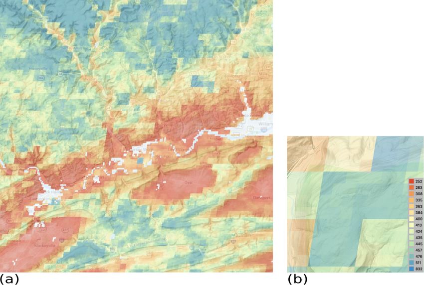
222                                                                              L. Poggio et al.: Soil information for the globe

2.4     Hyper-parameter selection and cross-validation            random forest, but rather a cumulative probability distribu-
                                                                  tion of the soil property at each location and depth.
Figure 2 summarises the approach used for the selection of           For each property (see Table 1) and standard depth from
the model hyper-parameters and the cross-validation. Further      the GlobalSoilMap specification (0–5, 5–15, 15–30, 30–60,
details are provided in the following sections.                   60–100 and 100–200 cm), four different values were com-
                                                                  puted to characterise this distribution: median (0.50 quantile,
2.4.1    Model tuning and numeric evaluation                      q0.50 ), mean, 0.05 quantile (q0.05 ) and 0.95 quantile (q0.95 ),
                                                                  i.e. the lower and upper limits of a 90 % prediction inter-
Model tuning was performed with a 10-fold cross-validation
                                                                  val. This uncertainty interval is as described in the Global-
procedure applied to multiple combinations of hyper-
                                                                  SoilMap specifications (Arrouays et al., 2014). The predic-
parameters.
                                                                  tions were computed for the mid-point of the depth interval
   Different numbers of decision trees (ntree parameter) were
                                                                  and considered constant for the whole depth interval.
combined with different numbers of covariates used in tree
                                                                     In order to compute the prediction uncertainty for soil tex-
splits (mtry parameter). The number of trees was progres-
                                                                  ture, the back-transformation was applied at the level of indi-
sively increased with the following values: 100, 150, 200,
                                                                  vidual tree predictions and the quantiles of the tree prediction
250, 500, 750 and 1000. The different mtry values were mul-
                                                                  distributions obtained from the resulting values.
tiples of the square root of the number of covariates. Four
multipliers were tested, 1 (default in ranger), 1.5, 2 and
3. For example, if the RFE procedure identified a set of 50       2.5.2    Uncertainty
covariates, the mtry values assessed were 7, 11, 14 and 21.       The percentage of cross-validation observations contained
   Each of the resulting combinations of ntree and mtry pa-       in the 0.9 prediction interval was calculated (prediction in-
rameters was used to train a different model with observa-        terval coverage probability, PICP) (Shrestha and Soloma-
tions from nine folds. Predictions were then assessed on the      tine, 2006). Ideally the PICP is close to 0.9, indicating that
remaining fold with classical performance measures, i.e. root     the uncertainty was correctly assessed. A PICP substantially
mean squared error (RMSE) and model efficiency coefficient        greater than 0.9 suggests that the uncertainty was underes-
(MEC; Janssen and Heuberger, 1995). MEC is equal to the           timated; a substantially smaller PICP indicates that it was
fraction of the explained variance based on the 1 : 1 line of     overestimated.
predicted versus observed that is defined as 1 minus the ratio       Furthermore, to visualise the uncertainty as a map, the fol-
between residual sum of squares and total sum of squares.         lowing indicators were calculated:
The final hyper-parameter selection was based on an optimi-
sation of model performance and computational constraints,          1. 90th prediction interval (PI90)
in this case memory consumption. For example an increase
                                                                        PI90 = q0.95 − q0.05 ;                                 (2)
of the ntree parameter above 200 provided a minor increment
in the metrics (usually less than 0.1 %, not reported here)
                                                                    2. ratio of the interquartile range over the median (predic-
while requiring considerably more memory and computation
                                                                       tion interval ratio, PIR):
time.
   The model evaluation was based on the performance met-                       q0.95 − q0.05
                                                                        PIR =                 .                                (3)
rics of the selected hyper-parameters’ combination. Predic-                         q0.50
tions at the centre of the six standard depth intervals were
compared with observations having the midpoint included           2.6     Qualitative evaluation of spatial patterns
within the considered interval.
                                                                  Expert judgement was used to evaluate the reasonableness
                                                                  of the maps, by comparing well-known spatial patterns at
2.5     Prediction and uncertainty quantification
                                                                  global, regional and local scales with SoilGrids predictions
2.5.1    Model fit                                                (see Sect. 3.4). Obviously these are not definitive evaluations,
                                                                  only indicative.
The final model for each soil property was fitted with all
available observations, the covariates and the hyperparam-
                                                                  2.7     Software and computational framework
eters selected in the previous steps. Observation depth was
included in the model as a covariate. It was calculated at the    SoilGrids requires an intensive computational workflow,
midpoint of the sampled layer or horizon.                         with numerous steps integrating different software. Soil-
   Models were obtained with the ranger package (Wright           Grids is entirely based on open-source software, in particular
and Ziegler, 2017), with the option quantreg to build             SLURM (Yoo et al., 2003) for job management, GRASS GIS
quantile random forests (QRF; Meinshausen, 2006). With            (GRASS Development Team, 2020) for data and tiles’ man-
this option, the prediction is not a single value, e.g. the av-   agement and R statistical software (R Core Team, 2020) for
erage of predictions from the group of decision trees in the      model fitting and statistical analysis.

SOIL, 7, 217–240, 2021                                                                  https://doi.org/10.5194/soil-7-217-2021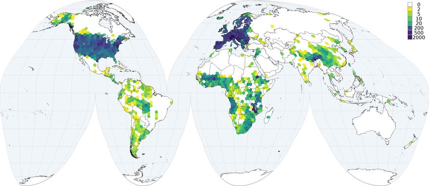
L. Poggio et al.: Soil information for the globe                                                                                  223

Figure 2. Detailed workflow for the Hyper-parameter selection and cross-validation.

   Predictions were computed in a high-performance com-                    As indicated, the number of observations for each property
puting cluster. A dynamic geographic tiling system was de-             varies greatly with depth and bioclimatic region, with higher
veloped with GRASS GIS to maximise the use of memory                   densities observed for North America and Europe. Generally,
for each job. Technical details on this parallelisation scheme         there are more observations for agricultural areas. Further,
are given in de Sousa et al. (2020).                                   the available profiles have been collated over several decades,
   The predictions were multiplied by a conversion factor of           some 62 % of the data being from 1960–2020; the time of
10 or 100 to maintain the required precision while using in-           sampling is unknown for around 34 % of the profiles. As in-
teger type in the file geotiff to reduce space occupied on disk.       dicated by Batjes et al. (2020), in principle, the age of the
Application of the conversion factor resulted in mapped lay-           observations should be taken into account during the map-
ers with units differing from those of the input observations          ping process via covariate layers for time periods commen-
(see Table 1).                                                         surate with the sampling dates, especially for soil properties
   The total computation time with the selected covariates             that are readily affected by changes in land use or manage-
and hyper-parameters differed per property. On average, the            ment practices. However, for these so-called “dynamic” soil
complete computation of the 24 maps (mean and three quan-              properties, such as pH and soil organic matter content, we
tiles for each of the six standard depths) for a single prop-          consider that the spatial variation will be much greater that
erty, including (i) RFE, (ii) model training and (iii) predic-         the temporal variation, so that not taking the age of observa-
tion, took approximately 1500 CPU hours. The prediction ac-            tions into account will not greatly affect the map. In addition,
counted for about two-thirds of the total time.                        it is difficult or impossible to find comparable covariates, in
                                                                       particular remote-sensing-derived covariates, for each time
                                                                       period. Space–time relations should be considered in future
3     Results and discussion                                           assessments (Heuvelink et al., 2020).
                                                                           This study considers standardised data for some 240 000
3.1    Input soil observations                                         profiles, derived from WoSIS. This is over 60 000 more pro-
                                                                       files than considered in the data compilation underpinning
Table 2 breaks down the distribution of the legacy soil ob-
                                                                       the preceding SoilGrids runs (Hengl et al., 2017b), thus pro-
servations for each soil property by depth interval. Table B1,
                                                                       viding substantial new information for calibration of the new
in Appendix B, shows the number of observations by biocli-
                                                                       global models. However, as indicated, there are still signif-
matic region.
                                                                       icant geographic gaps (e.g. arid regions, boreal regions and
   Figures 3 and 4 show examples of observation density of
                                                                       “forest” soils). Some of these are related to the physical re-
the soil calibration data for two soil properties, pHwater and
                                                                       moteness or inaccessibility of some regions, while others are
proportion of coarse fragments, that show a large difference
                                                                       related to the fact that many soil datasets still are not or can
in density.

https://doi.org/10.5194/soil-7-217-2021                                                                     SOIL, 7, 217–240, 2021
224                                                                              L. Poggio et al.: Soil information for the globe

not be shared for various reasons as described by Arrouays         mum of 0.31 for coarse fragments to a maximum of 0.74
et al. (2017).                                                     for BDOD. Clay is less well modelled than the other two
   In the previous version of SoilGrids (Hengl et al., 2017b),     particle-size classes. This may be an effect of the chosen
synthetic observations were randomly placed in regions with        ALR transformation that had clay as denominator (Lark and
few or no observations, e.g. the Sahara and the Arabian            Bishop, 2007). Metrics of the mean were always better than
Peninsula. This approach is worth further exploring, includ-       or equal to those for the median for all properties.
ing information derived from other regional datasets, expert          Overall, these metrics are in line with continental or large-
opinion and transfer learning from similar areas according to      region DSM studies (Keskin and Grunwald, 2018). However,
the Homosoil concept (Mallavan et al., 2010), which assumes        they are slightly lower than those presented by Hengl et al.
similarity of soil-forming factors across regions. However,        (2017b). The latter difference can be explained by the more
SoilGrids already implicitly incorporates the Homosoil con-        prudent cross-validation approach now taken, with spatially
cept, as long as there are sufficient observations in a given      balanced folds and all observations belonging to the same
soil-forming environment anywhere in the world. Therefore,         profile in the same fold. This prevents the use of data from the
no synthetic observations (“pseudo-points”) were included in       same profile both for calibration and numerical evaluation.
this version of SoilGrids, also by a lack of confidence about         Table 4 shows that the models with a higher number of
the accuracy of the synthetic data.                                retained covariates (Table 3) have better predictive perfor-
   In future studies, it will be relevant to identify beforehand   mances. However, these models are also the models with the
areas of the world with a low observation density that are not     largest number of observations (Table 2). The considered soil
yet represented by a high density of observations in other         properties are also different. Therefore, no general conclu-
areas with similar soil-forming factors. A set of synthetic        sion can be drawn from this observation.
profiles could then be generated to describe these areas, by          Table 5 shows the MEC for mean predictions by depth in-
consulting soil scientists knowledgeable on the soils and soil     terval. Performances decreased with depth, in line with many
properties of these areas.                                         other DSM studies (Keskin and Grunwald, 2018). This pat-
                                                                   tern can be explained mainly by weakened relationships be-
3.2   Model tuning and hyper-parameter selection
                                                                   tween environmental layers and soil properties of the deeper
                                                                   layers.
Model hyper-parameters selected for each property are pre-            In this study, the vertical dimension of soil variability was
sented in Table 3.                                                 only taken into account by using the depth of the observa-
   The numbers of covariates selected using the two-step ap-       tion as a covariate. Recent publications (Ma et al., 2021;
proach for covariates’ selection was fairly small in compari-      Nauman and Duniway, 2019) indicate that such an approach
son with the full set (Table 3), resulting in more parsimonious    can be too simplistic or lead to problems with consistency
models. Figure 5 shows two examples of the loss function for       over the predicted depth sequence. This may be true for lo-
RFE for two soil properties with different numbers and distri-     cal datasets, in which the short-range spatial variability is
butions of input observations. In both cases, there is a clear     of a similar magnitude as the vertical variability. Further re-
improvement of performances while using 15 to 20 covari-           search is necessary to assess the effects of using depth as a
ates. The curve reaches a minimum of the loss function and         covariate on global datasets and models. Alternatives such
then stays on a plateau with a slight decline after the identi-    as 3D smoothers (Poggio and Gimona, 2017b) or geostatis-
fied minimum.                                                      tical models exploiting 3D spatial auto-correlation are worth
   All final models were trained with a maximum of 200 de-         exploring in further studies.
cision trees, a number beyond which performance gains did             Table 6 summarises the PICPs, globally and by predicted
not noticeably increase.                                           depth interval. Most of the values are between 0.88 and 0.92,
   The mtry parameter mainly depended on the number of co-         indicating that the prediction intervals obtained with QRF are
variates and was always between 1.5 and 2 times the square         a realistic representation of the prediction uncertainty, as the
root of the number of covariates, which is the default pro-        expected value for a 90 % prediction interval is 0.90. Excep-
vided by common random forest packages such as ranger              tions are the models for coarse fragments with higher values
(Wright and Ziegler, 2017). This confirms the need to de-          around 0.95, indicating an overestimation of prediction un-
termine optimum model hyper-parameters, especially when            certainty. The texture components have values with a larger
dealing with large numbers of input data (Nussbaum et al.,         spread, around 0.78 to 0.80 for sand and closer to 0.96 for silt
2018) as is the case here.                                         and clay. These indicate a potential underestimation of pre-
                                                                   diction intervals for sand and overestimation for silt and clay.
3.3   Quantitative evaluation
                                                                   These results may be related with the range of these prop-
                                                                   erties in the input observations. The transformation method
Cross-validation results are summarised in Table 4, present-       used to derive the prediction intervals for the texture compo-
ing the root mean squared error (RMSE) and model effi-             nents could also be a contributing factor. Further exploration
ciency coefficient (MEC). The MEC varies from a mini-              of the causes is worthwhile.

SOIL, 7, 217–240, 2021                                                                 https://doi.org/10.5194/soil-7-217-2021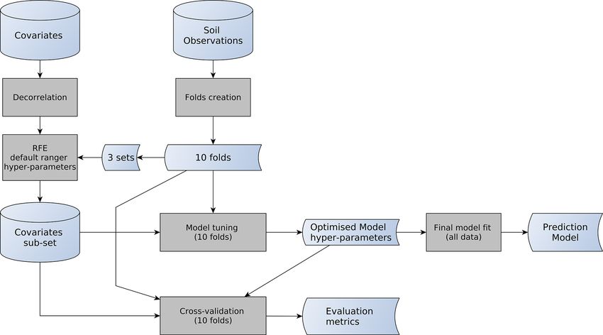
L. Poggio et al.: Soil information for the globe                                                                                        225

Table 2. Number of observations per standard depth interval for each soil property. See Table 1 for abbreviations and units of the soil
properties considered.

                          Depth interval     BDOD        CEC      CFVO            N       pH       SOC         STF
                          0–5 cm              8122      20 576    15 541    27192      44 049    48 616     42 983
                          5–15 cm            19 817     49 463    66 833    82 856    146 677   148 918    155 302
                          15–30 cm           17 819     40 673    35 254    39 568     91 326    91 682     98 659
                          30–60 cm           27 146     63 444    56 755    48 804    141 812   122 338    140 353
                          60–100 cm          23 130     58 038    50 912    36 946    131 172   102 687    12 7073
                          100–200 cm         23 396     66 236    49 995    28 135    129 373    92 327    116 847

Figure 3. Number of observations per grid cell (70 000 km2 ) for soil pHwater .

Table 3. Hyper-parameters for each considered soil property. See           known sampling design (Brus et al., 2011; Brus, 2014). How-
Table 1 for abbreviations and units of the soil properties considered.     ever, this is not feasible when only legacy data are available.
                                                                           In this case, a so-called “cross-validation” approach is often
                           Number of       Number of     mtry              used. This needs to be tuned to avoid over- or underestima-
                           covariates          trees                       tion of the numeric evaluation metrics, especially in case of
       BDOD                         40           200       12              large differences in observation density, i.e. clustered spatial
       CEC                          25           200       10              observations. This is especially important at global scale, as
       CFVO                         20           200        6              the distribution of the soil observations is not uniform across
       N                            30           200       10              the globe. It can not be guaranteed that the numeric evalua-
       pH                           32           200        9              tion metrics derived from cross-validation are unbiased esti-
       SOC                          40           200       12              mates of the true numeric evaluation metrics, i.e. those that
       Texture ALR I                25           150       10              would have been computed on a probability sample of the
       Texture ALR II               27           150       10              whole population. It is also not possible to quantify how close
                                                                           the cross-validation metrics estimates are to the true metrics,
                                                                           as it is not possible to obtain confidence intervals (Brus et al.,
   A key issue for DSM applications using legacy soil data is              2011). When using cross-validation it is important to pre-
the evaluation of the results. The aspect of evaluation which              vent over- or under-optimistic estimates. For example, it is
compares actual with predicted values is numerical (or sta-                likely that prediction errors are smaller in areas where the
tistical) evaluation, often termed “validation” in the DSM lit-            sampling density is higher. Because of their high sampling
erature; Oreskes (1998) and Rossiter (2017) explain why the                density, such areas will be over-represented in the sample
term “evaluation” is preferred for the overall process of as-              as the percentage of cross-validation points in clustered ar-
sessing the success of models, including DSM models. The                   eas will be higher than the percentage of the total land area
best approach to numerical evaluation is to have an inde-                  covered by those areas. Results of standard cross-validation
pendent dataset obtained with probability sampling using a                 will be strongly influenced by the performances in clustered

https://doi.org/10.5194/soil-7-217-2021                                                                          SOIL, 7, 217–240, 2021
226 L. Poggio et al.: Soil information for the globe Figure 4. Number of observations per grid cell (70 000 km2 ) for coarse fragments. Figure 5. Example of loss function (RMSE) used in the RFE step of covariates’ selection. areas. Using spatial cross-validation as suggested by Meyer been applied with success in other geostatistics exercises and et al. (e.g. 2018), where it is ensured that calibration data are could be adapted to global soil mapping. The creation of the never too close to a cross-validation point, on the other hand folds could also be modified to take into account the density could produce over-pessimistic results. In order to address of the observations. some of these concerns, this study adopted a practical solu- tion in which the folds were created to guarantee a spatially balanced distribution between cross-validation folds, main- 3.4 Qualitative evaluation of spatial patterns taining the same densities of the input data in each fold so At global scale, well-known patterns are reproduced, and that they represent approximately the same population. typical properties associated with many World Reference Although the numerical evaluation procedure used in this Base for Soil Resources (WRB) (IUSS Working Group work takes into account the spatial distribution of the ob- WRB, 2015) Reference Soil Groups can be recognised. servations and their density, further improvement is possi- For example, the pH map identifies the large regions of ble in both model training and evaluation. For example, the alkaline soils (Solonetz, Solochak), highly weathered soils weights assigned to observations in heavily sampled areas (e.g. Acrisols, Alisols, Plithosols), acid forest soils (e.g. Pod- could be reduced. The United States and large regions of Eu- zols) and young soils from calcareous glacial deposits (e.g. rope and Australia have high numbers of observations that Luvisols). The low pH of Andosols (e.g. Pacific North- could be downweighted to strengthen the spatial robustness west United States, Japan, New Zealand) is also correctly of the evaluation procedure. Declustering or debiasing tech- represented. The texture components (particle size class – niques (Goovaerts, 1997; Deutsch and Journel, 1998) have PSC) maps correctly identify the siltier deltas (e.g. Yellow– SOIL, 7, 217–240, 2021 https://doi.org/10.5194/soil-7-217-2021
L. Poggio et al.: Soil information for the globe                                                                                        227

Table 4. Global cross-validation results for both mean and median predictions. See Table 1 for abbreviations and units of the soil properties
considered.

                           Property    RMSE (median)       RMSE (mean)       MEC (median)       MEC (mean)
                           BDOD                     0.19              0.19              0.73             0.74
                           CEC                     11.01             10.69              0.40             0.43
                           CFVO                    13.46             12.69              0.22             0.31
                           N                        2.62              2.50              0.47             0.52
                           pH                       0.78              0.77              0.67             0.68
                           SOC                     39.67             36.48              0.37             0.47
                           Sand                     0.19              0.18              0.51             0.54
                           Silt                     0.13              0.13              0.60             0.62
                           Clay                     0.13              0.13              0.42             0.43

Table 5. MEC per depth layer for mean predictions. See Table 1 for abbreviations and units of the soil properties considered.

                         Depth layer     BDOD       CEC     CFVO        N      pH    SOC       Sand    Silt     Clay
                         0–5 cm             0.78    0.46      0.33    0.65    0.69    0.55     0.59   0.71      0.45
                         5–15 cm            0.74    0.42      0.35    0.41    0.66    0.39     0.58   0.64      0.42
                         15–30 cm           0.72    0.39      0.33    0.44    0.68    0.38     0.57   0.68      0.42
                         30–60 cm           0.70    0.42      0.31    0.46    0.68    0.38     0.54   0.62      0.41
                         60–100 cm          0.61    0.41      0.29    0.48    0.68    0.42     0.50   0.57      0.40
                         100–200 cm         0.59    0.45      0.29    0.49    0.67    0.59     0.48   0.54      0.40

Yangtze, Ganges–Brahmaputra), broad river plains (e.g. Po,                  However, at the local scale, a preliminary assessment of
Danube, Mississippi, Rio Plate, upper Amazon), the loess re-             SoilGrids in the United States, compared with a gridded ver-
gions (e.g. Midwestern United States, NW Europe, Ukraine)                sion of the national detailed gSSURGO (NRCS National Soil
and the sandy North German–Polish plain. The cation ex-                  Survey Center, 2016) soil geographic database based on a de-
change capacity (CEC) map clearly identifies large regions of            tailed field survey, reveals that SoilGrids may fail to account
highly weathered clays (e.g. Southeastern United States and              for local parent material transitions, e.g. sedimentary facies
China, central Brazil) and high-CEC 2 : 1 clays (e.g. “black             of coastal plain marine sediments, as well as glacial features
cotton” Vertisols in the Deccan plateau and the Sudan). This             such as proglacial lacustrine sediments and relic beach lines,
map, together with the soil organic carbon (SOC) concentra-              so that the local PSC pattern is not accurate, sometimes on
tion maps, identifies large regions of Histosols (e.g. north-            the order of 20 %–30 % of a particle-size class.
ern Canada, Scotland, Siberia, Borneo). The SOC stock map                   For example, Fig. 6a shows predicted sand concentration
identifies deep Histosols and cool, wet regions (e.g. Pacific            of the 0–5 cm layer in an approximately 50 × 50 km area in
Northwest North American coast, Ireland, southern Chile).                central Pennsylvania (United States), ranging from approxi-
The coarse fragment map identifies large areas of the Tibetan            mately 25 % (darkest red) to 80 % (darkest blue). Important
Plateau and the principal mountain chains, as well as recently           local differences are clear: the low sand concentrations of the
glaciated soils on igneous bedrock (e.g. Scandinavia, north-             clayey soils in the limestone valleys trending SW–NE and
ern Quebec and Ontario).                                                 the high concentrations in soils from glacial till developed
    Many regional patterns are also clear, for example the pH            on sandstones in the north, as well as the residual soils on the
transition from Sahara through Sahel to the West African                 resistant sandstone ridges of the Ridge and Valley province
coast and the PSC transitions from the Des Moines glacial                of Appalachia in the south. These do generally agree with the
lobe to the proglacial loess deposits in Iowa (United States)            detailed soil survey.
as well as the PSC transition from clayey marine sediments                  At the detailed scale (250 m pixel), SoilGrids typically
along the North and Baltic Sea coasts through the sandy                  shows fine details that do not always appear to be related
plains to the central German loess belt. The CEC map iden-               to obvious landscape or land use differences, when the map
tifies contrasting areas of Vertisols (e.g, “black belts” in             is viewed as a ground overlay in Google Earth. For example,
Alabama–Mississippi and Texas, United States). The coarse                Fig. 6b shows detail of predicted sand concentration of the 0–
fragment map shows the detailed pattern of the basin-and-                5 cm layer in an approximately 3 × 3 km area of the previous
range region of the western United States and the ridge-and-             figure. The effect of some covariates being at 1 km resolu-
valley region of Appalachia.                                             tion and others at 250 m is apparent, but the reason for the

https://doi.org/10.5194/soil-7-217-2021                                                                           SOIL, 7, 217–240, 2021
228 L. Poggio et al.: Soil information for the globe
Table 6. Prediction interval coverage probability, global and by predicted depth interval. See Table 1 for abbreviations and units of the soil
properties considered.
Property Global [0, 5] [5, 15] [15, 30] [30, 60] [60, 100] [100, 200]
BDOD 0.90 0.89 0.91 0.91 0.91 0.90 0.88
CEC 0.88 0.89 0.90 0.88 0.88 0.88 0.87
CFVO 0.95 0.96 0.95 0.95 0.95 0.94 0.94
N 0.92 0.91 0.92 0.93 0.92 0.92 0.92
pH 0.90 0.91 0.91 0.90 0.91 0.90 0.89
SOC 0.92 0.91 0.92 0.92 0.92 0.92 0.92
Sand 0.79 0.82 0.82 0.80 0.78 0.78 0.78
Silt 0.96 0.95 0.96 0.96 0.96 0.96 0.96
Clay 0.96 0.96 0.96 0.96 0.95 0.95 0.96
Figure 6. Predicted sand concentration, %, 0–5 cm, ground overlay in © Google Earth. (a) Overview; centre ≈ −77◦ 140 E, 41◦ 140 N, near
Jersey Shore, PA. (b) Detail; centre ≈ −76◦ 560 E, 41◦ 330 N.
fine-scale differences is not. This area is of similar lithology, 3.5 Prediction uncertainty
relief and land cover (second-growth dense forest) except the
narrow valley at the north-west edge, yet the predictions are In general, the least sampled areas present the highest pre-
quite different. diction uncertainties as expressed by the PICP. Figures 7
In this context, it should be realised that SoilGrids250m and 8 show an example for two properties and depths (maps
predictions are not meant for use at a detailed scale, i.e. at for all properties and depths can be accessed at https://data.
the subnational or local level, as national data providers of- isric.org). Figure 9 and 10 show an example representing the
ten have access to more detailed point datasets and covariate quantiles for pHwater for the 60–100 cm layer. The north of
layers for their country than have been provided to the point Russia and the centre and north-west of Canada are large re-
dataset on which SoilGrids250m is based (Chen et al., 2020; gions for which few soil observations are available; therefore
Roudier et al., 2020; Vitharana et al., 2019; Liu et al., 2020). prediction distributions are wider than in more densely sam-
pled areas. However, these patterns are different for different
properties. For example, arid areas actually have the narrow-
est prediction ranges of pHwater . The uncertainty range is of-
SOIL, 7, 217–240, 2021 https://doi.org/10.5194/soil-7-217-2021L. Poggio et al.: Soil information for the globe 229
ten wide for properties and regions with a wider range of the of the data support these highly complex models. This is the
property being modelled. This can be explained by the mod- case in particular with convolutional or recursive neural net-
elling approach performing more accurately within a limited works (deep learning). However, these methods present com-
range of options. These regions also have larger local spatial putational challenges with the amount of training data nec-
variation with more difficulties for predictions. essary for a sufficiently accurate DSM exercise, especially
The communication of uncertainty is an open challenge when working at global scale at medium to fine resolutions.
(Arrouays et al., 2020). Uncertainty should provide informa- Fourth, the proper method of cross-validation is an-
tion for policymakers and other stakeholders and not only other important aspect when considering how to assess and
scientists and modellers. The maps computed with Eq. (3) are improve model performances. In particular, spatial cross-
a first step in this direction, but their limitations must be un- validation and declustering of the data need to be further ex-
derstood. For properties that have values at or near zero, e.g. plored.
coarse fragments, they do not provide an entirely accurate Fifth, this research considered only the modelling of some
uncertainty estimate. The use of uncertainty classes could be primary soil properties, as defined and described in the Glob-
a further step to help domain stakeholders. alSoilMap specifications. More work is necessary to obtain
maps for soil thickness (either rooting zone, pedogenetic
3.6 Limitations and outlook
solum or regolith), soil properties derived with pedo-transfer
functions, e.g. hydrologic soil properties such as saturated
This study represents a considerable effort to provide a glob- hydraulic conductivity (Pachepsky and Rawls, 2004), and
ally consistent product using the point dataset available to IS- complex properties that depend on multiple primary prop-
RIC, a large number of relevant covariates and some optimi- erties, e.g. carbon stocks. These layers are important inputs
sation of a well-established machine learning method, within to model and map soil functions in the present and in the fu-
the limits of practical computation. Yet it is clear that this ture as well as to support Earth system modelling (Luo et al.,
product has some limitations, which will be considered in 2016; Dai et al., 2019).
further work. Sixth, the quantification of uncertainty is recommended
First, there is an ever-expanding group of new covari- and is becoming more common in DSM studies. This work
ates that can help explain and model the spatial variation introduced it at global scale for the first time to the best of our
of soil properties. Products derived from Earth observation knowledge. While the provision of quantiles is mentioned
are particularly relevant in this regard and have considerably in the GlobalSoilMap specifications, the representation and
improved over the last decade. For example, the European communication of uncertainty to end users and stakehold-
Space Agency Sentinel missions (both optical and radar) pro- ers remain an important research field to be further explored.
vide high-resolution data that have been shown to improve The appropriate uncertainty intervals, both in terms of user
DSM model performances. acceptance and modelling feasibility, also need to be investi-
Second, a fundamental problem is a lack of well dis- gated.
tributed point observations within the soil property geo- Finally, the integration of highly automatised workflows
graphic and features space. Additional soil data for so far with expert opinion should be further explored. DSM prod-
under-represented regions, for example the northern boreal ucts use statistical models to describe soils, and it is im-
regions as being collated by the International Soil Carbon portant to take into account the expertise and experience of
Network (Malhotra et al., 2019), will be sought for possible pedologists, at least in an evaluation loop if not as part of the
consideration in the WoSIS workflow that provides the point modelling itself. We made a first attempt at this in the Qual-
data underpinning the SoilGrids mapping effort. This effort itative evaluation section above but do not have a method to
would be aided by the provision by more data providers of at effectively incorporate expert observations into a workflow.
least a representative part of their point data to WoSIS, under
suitable license. It is also important to consider the distribu-
tion of the observations in the covariate space to minimise the 4 Conclusions
issues related to predictions into unknown regions of feature
space (Meyer and Pebesma, 2020). This study presents and discusses the production of global
Third, DSM methods are under active development, both maps of soil properties as implemented in the SoilGrids
new methods and improvements to established methods. The 2.0 product, with cross-validation, hyper-parameter selection
use of decision-tree-based models in DSM has become fairly and quantification of uncertainty, using the best available
common in recent years. Models such as random forests, (shared) soil profile data for the world. In particular, the study
XGBoost or Cubist tend to provide better results than most describes a robust and reproducible DSM workflow address-
multiple linear regression methods with reasonable computa- ing the challenges of global data modelling:
tion costs (Khaledian and Miller, 2020). However, methods
such as artificial neural networks promise further improve- 1. non-homogeneous spatial distribution of input soil ob-
ments in model performances if the amount and distribution servations;
https://doi.org/10.5194/soil-7-217-2021 SOIL, 7, 217–240, 2021230 L. Poggio et al.: Soil information for the globe Figure 7. Mean soil organic carbon content (dg/kg) prediction and range between 5 % and 95 % quantiles in the 5 to 15 cm depth interval, (a) for prediction and (b) for interquartile range. Figure 8. Median total nitrogen prediction (cg/kg) and associated uncertainty for the 15 to 30 cm depth interval, (a) for prediction and (b) for uncertainty. SOIL, 7, 217–240, 2021 https://doi.org/10.5194/soil-7-217-2021
L. Poggio et al.: Soil information for the globe                                                                                         231

Figure 9. Prediction distribution for pHwater (10 pH) in the 60 to 100 cm depth interval, (a) for mean and (b) for median.

Figure 10. Prediction distribution for pHwater (10 pH) in the 60 to 100 cm depth interval, (a) for 5 % quantile and (b) for 95 % quantile.

https://doi.org/10.5194/soil-7-217-2021                                                                          SOIL, 7, 217–240, 2021
232                                                               L. Poggio et al.: Soil information for the globe

 2. robust quantitative evaluation with a cross-validation
    procedure balancing accuracy and performances;
 3. qualitative evaluation of the spatial patterns of the maps
    to include information about matching with well recog-
    nised pedo-landscape features;
 4. quantification and mapping of the spatial uncertainty to
    provide users with a measure for and warning for users
    of the products.
   As such, it describes a next step into global modelling and
mapping of soil properties, explicitly highlighting the im-
portance of quantitative and qualitative evaluation and un-
certainty communication. The actual use of SoilGrids 2.0 in
global and wide-area regional applications, where soil prop-
erties are important model inputs, will be the real test of its
applicability and usefulness.

SOIL, 7, 217–240, 2021                                                  https://doi.org/10.5194/soil-7-217-2021
L. Poggio et al.: Soil information for the globe 233
Appendix A: Environmental covariates
Over 400 geographic layers were available as environmental
covariates for this work. These are chosen for their presumed
relation to the major soil forming factors.
Table A1. Covariate sets and sources.
Weather and climate
- Temperature and precipitation from the Climatologies at high resolution for the Earth’s land surface areas (CHELSEA)
dataset (Karger et al., 2016)
- Snowfall from ESA’s CCI Land Cover dataset (Bontemps et al., 2013)
- Cloud cover by EarthEnv (Wilson and Jetz, 2016)
- Temperature and water vapour from NASA’s MODIS products (Wan, 2006)
- Precipitation, solar radiation, temperature, water vapour, wind speed plus various indexes from the WorldClim version 2
climate data series (Fick and Hijmans, 2017)
Ecology and ecosystems
- Bioclimatic zones in the Global Ecophysiography product by the USGS Geosciences and Environmental Change Science
Center (GECSC) (Dinerstein et al., 2017)
Geology
- Average soil and sedimentary-deposit thickness by the Distributed Active Archive Centre (DAAC) (Pelletier et al., 2016).
- Rock types by the USGS Geosciences and Environmental Change Science Center (GECSC), based on the Global Lithological
Map database v1.1 (Hartmann and Moosdorf, 2012)
Land use and land cover
- 2010 land cover classes from ESA’s CCI Land Cover (Bontemps et al., 2013)
- Bare ground and tree cover from the USGU Global Land Cover dataset (Hansen et al., 2013)
- 2010 land cover classes from the NGCC’s GLobeLand30 product (Chen et al., 2015)
Elevation and morphology
- Land surface elevation from the EarthEnv-DEM90 dataset (Robinson et al., 2014)
- Land surface elevation and various morphology indexes from the WorldGrids dataset (Reuter and Hengl, 2012)
- Land form classes in the Global Ecophysiography product by the USGS Geosciences and Environmental Change Science
Center (GECSC) (Sayre et al., 2014)
Core satellite outputs
- Bands 3, 4, 5 and 7 from Landsat (Zanter, 2019)
- Middle- and near-infrared bands from MODIS (Savtchenko et al., 2004)
Vegetation indexes
- NDVI from Landsat (Zanter, 2019)
- EVI and NPP from MODIS (Savtchenko et al., 2004)
Hydrography
- Global Inundation Extent from Multi-Satellites (GIEMS) dataset by Estellus (Fluet-Chouinard et al., 2015)
- Extent of glaciers, surface water change and occurrence probability by the JRC (Pekel et al., 2016)
- Global water table depth (Fan et al., 2013)
https://doi.org/10.5194/soil-7-217-2021 SOIL, 7, 217–240, 2021234 L. Poggio et al.: Soil information for the globe
Appendix B: Bioclimatic regions
Table B1 summarises the number of observations per prop-
erty for each bioclimatic region. An interactive map of the re-
gions is available at http://ecoregions2017.appspot.com/ (last
access: 20 May 2021).
Table B1. Number of observations per property for each bioclimatic region. See Table 1 for abbreviations.
Biome CEC CFVO N pH SOC STF
Tropical and subtropical moist broadleaf forests 4185 2117 8378 12 872 11 901 11 651
Tropical and subtropical dry broadleaf forests 558 205 1370 3264 2724 3051
Tropical and subtropical coniferous forests 59 30 54 1336 878 1331
Temperate broadleaf and mixed forests 12 585 29 708 24 711 56 569 49 727 61 822
Temperate conifer forests 6058 6417 5812 7597 9490 9834
Boreal forests/taiga 1443 3210 4834 4140 6819 5358
Tropical and subtropical grasslands, savannas and shrublands 8391 8259 20 181 27 633 24 951 23 135
Temperate grasslands, savannas and shrublands 13 442 9885 9812 23 654 24 421 25 416
Flooded grasslands and savannas 246 124 503 754 818 798
Montane grasslands and shrublands 479 1865 1073 1386 3994 3568
Tundra 312 199 466 548 807 695
Mediterranean forests, woodlands and scrub 1747 5951 8034 9126 12 532 11 428
Deserts and Xeric shrublands 3342 3412 3224 8994 8163 9862
Mangroves 88 26 165 264 437 250
SOIL, 7, 217–240, 2021 https://doi.org/10.5194/soil-7-217-2021L. Poggio et al.: Soil information for the globe 235
Code and data availability. The code underpinning the Soil- Review statement. This paper was edited by Nicolas P. A. Saby
Grids 2.0 workflow is available under the GPL3 license at https: and reviewed by Feng Liu and Dominique Arrouays.
//git.wur.nl/isric/soilgrids/soilgrids (last access: 21 May 2021).
SoilGrids predictions themselves are available to the public un-
der the Creative Commons CC-BY 4.0 licence, facilitating their
widespread use. They may be obtained as world mosaics in the Vir- References
tual Raster Tile (VRT) format from https://files.isric.org/soilgrids/
latest/ (last access: 21 May 2021). The Web Coverage Service Aitchison, J.: The statistical analysis of compositional data, Chap-
(WCS; https://maps.isric.org, last access: 21 May 2021) facilitates man & Hall, London, UK, 1986.
automated access, e.g. from computer programmes or modelling Akpa, S. I. C., Odeh, I. O. A., Bishop, T. F. A., and
frameworks. A set of notebooks (https://git.wur.nl/isric/soilgrids/ Hartemink, A. E.: Digital Mapping of Soil Particle-
soilgrids.notebooks, last access: 21 May 2021) was developed with Size Fractions for Nigeria, Soil Sci., 78, 1953–1966,
examples for the use of the WCS. A new web-based portal (https: https://doi.org/10.2136/sssaj2014.05.0202, 2014.
//soilgrids.org/, last access: 21 May 2021) was also developed with Arrouays, D., Grundy, M. G., Hartemink, A. E., Hempel, J. W.,
this release, providing users with a light and swift means to visualise Heuvelink, G. B., Hong, S. Y., Lagacherie, P., Lelyk, G.,
and explore the new predictions, making the best of state-of-the-art McBratney, A. B., McKenzie, N. J., de Lourdes Mendonca-
technologies for the web. A ReST API in beta stage is also available Santos, M., Minasny, B., Montanarella, L., Odeh, I. O.,
at https://rest.soilgrids.org/ (last access: 21 May 2021). Sanchez, P. A., Thompson, J. A., and Zhang, G.-L.: Global-
SoilMap: Toward a Fine-Resolution Global Grid of Soil Prop-
erties, in: Advances in Agronomy, Academic Press, 93–134,
Supplement. The supplement related to this article is available https://doi.org/10.1016/B978-0-12-800137-0.00003-0, 2014.
online at: https://doi.org/10.5194/soil-7-217-2021-supplement. Arrouays, D., Leenaars, J. G. B., Richer-de Forges, A. C., Ad-
hikari, K., Ballabio, C., Greve, M., Grundy, M., Guerrero, E.,
Hempel, J., Hengl, T., Heuvelink, G., Batjes, N., Carvalho, E.,
Hartemink, A., Hewitt, A., Hong, S.-Y., Krasilnikov, P., La-
Author contributions. LP and LMdS conceived and executed the
gacherie, P., Lelyk, G., Libohova, Z., Lilly, A., McBratney, A.,
research and wrote the paper. NHB, GBMH and BK gave sugges-
McKenzie, N., Vasquez, G. M., Mulder, V. L., Minasny, B., Mon-
tions about the approach and contributed extensively to the paper.
tanarella, L., Odeh, I., Padarian, J., Poggio, L., Roudier, P., Saby,
DR designed and executed the qualitative evaluation and wrote the
N., Savin, I., Searle, R., Solbovoy, V., Thompson, J., Smith, S.,
corresponding sections in the paper. NHB and ER designed and cre-
Sulaeman, Y., Vintila, R., Rossel, R. V., Wilson, P., Zhang, G.-L.,
ated the database of soil observations. All authors reviewed the pa-
Swerts, M., Oorts, K., Karklins, A., Feng, L., Ibelles Navarro,
per.
A. R., Levin, A., Laktionova, T., Dell’Acqua, M., Suvannang,
N., Ruam, W., Prasad, J., Patil, N., Husnjak, S., Pásztor, L.,
Okx, J., Hallet, S., Keay, C., Farewell, T., Lilja, H., Juilleret,
Competing interests. The authors declare that they have no con- J., Marx, S., Takata, Y., Kazuyuki, Y., Mansuy, N., Panagos,
flict of interest. P., Van Liedekerke, M., Skalsky, R., Sobocka, J., Kobza, J.,
Eftekhari, K., Alavipanah, S. K., Moussadek, R., Badraoui, M.,
Da Silva, M., Paterson, G., Gonçalves, M. D. C., Theocharopou-
Acknowledgements. We thank Rik van den Bosch (ISRIC Di- los, S., Yemefack, M., Tedou, S., Vrscaj, B., Grob, U., Kozák,
rector) for the internal support to the SoilGrids project. We espe- J., Boruvka, L., Dobos, E., Taboada, M., Moretti, L., and Ro-
cially thank the organisations and experts (https://www.isric.org/ driguez, D.: Soil legacy data rescue via GlobalSoilMap and
explore/wosis/wosis-contributing-institutions-and-experts, last ac- other international and national initiatives, GeoResJ, 14, 1–19,
cess: 21 May 2021) that provided soil point data for consideration https://doi.org/10.1016/j.grj.2017.06.001, 2017.
in WoSIS and SoilGrids. Laura Poggio is a member of a consor- Arrouays, D., McBratney, A., Bouma, J., Libohova, Z., de Forges,
tium supported by LE STUDIUM Loire Valley Institute for Ad- A. C. R., Morgan, C. L., Roudier, P., Poggio, L., and Mulder,
vanced Studies through its LE STUDIUM Research Consortium V. L.: Impressions of digital soil maps: The good, the not so
Programme. good, and making them ever better, Geoderma Regional, 20,
e00255, https://doi.org/10.1016/j.geodrs.2020.e00255, 2020.
Ballabio, C., Panagos, P., and Monatanarella, L.: Mapping topsoil
Financial support. This work was supported by ISRIC core fund- physical properties at European scale using the LUCAS database,
ing, with additional support from the European Union’s EU H2020 Geoderma, 261, 110–123, 2016.
Research and Innovation Programme, grant agreement no. 774378 Banwart, S., Black, H., Cai, Z., Gicheru, P., Joosten, H., Victo-
(https://www.circasa-project.eu, last access: 21 May 2021). ISRIC ria, R., Milne, E., Noellemeyer, E., Pascual, U., Nziguheba,
– World Soil Information, legally registered as the International Soil G., Vargas, R., Bationo, A., Buschiazzo, D., de Brogniez, D.,
Reference and Information Centre, receives core funding from the Melillo, J., Richter, D., Termansen, M., van Noordwijk, M., Go-
Netherlands Government. verse, T., Ballabio, C., Bhattacharyya, T., Goldhaber, M., Niko-
laidis, N., Zhao, Y., Funk, R., Duffy, C., Pan, G., la Scala, N.,
Gottschalk, P., Batjes, N., Six, J., van Wesemael, B., Stocking,
M., Bampa, F., Bernoux, M., Feller, C., Lemanceau, P., and Mon-
tanarella, L.: Benefits of soil carbon: report on the outcomes of
https://doi.org/10.5194/soil-7-217-2021 SOIL, 7, 217–240, 2021You can also read