Space-discretizations of reaction-diffusion SPDEs - Carina Geldhauser Lund University joint work with - FAUbox
←
→
Page content transcription
If your browser does not render page correctly, please read the page content below
Space-discretizations of reaction-diffusion SPDEs

                                Carina Geldhauser
                                  Lund University

                                   joint work with
                      A.Bovier (Bonn), Ch. Kuehn (TU Munich)

Carina Geldhauser (Lund)            Discrete SPDEs             FAU-DCN 2021   1 / 23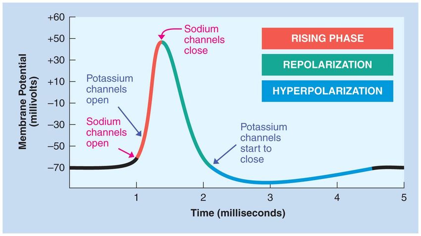
Why study discrete-in-space (S)PDEs?
Reason 1: they appear in nature

       myelinated nerve fibres
       formation of shear bands in granular flows
       enhancement of digital images
       chemotactic movement of bacteria
       (reinforced random walks on lattices)
                                                      Figure: Shear bands in dry
       population models                              granular media, Fazekas,
                                                      Török, Kertesz and Wolf, 2006

Reason 2: it really makes a difference
     an inherent discrete spatial structure can influence the dynamical
     behaviour of the physical/chemical/biological system
     the continuous equation may admit special solutions which the
     discrete equation does not have

   Carina Geldhauser (Lund)       Discrete SPDEs                 FAU-DCN 2021           2 / 23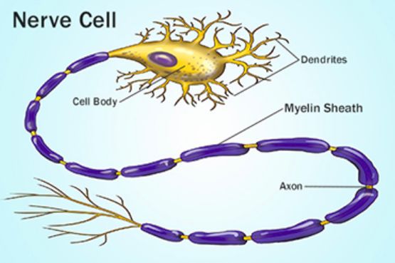
...but also noise may cause new phenomena: metastability

Examples of metastable systems

         undercooled destilled water
         conformations of proteins
         stock prices in ”overheated” markets

 Figure: Energies levels of conformations of
 cyclohexane                                               Figure: Adams and Vanden-Eijnden, PNAS 2010:
                                                           counterrotation of HIV-1 gp120

    Carina Geldhauser (Lund)                   Discrete SPDEs                           FAU-DCN 2021      3 / 23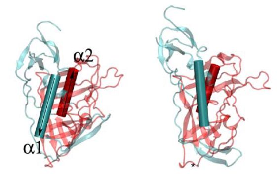
Outline

1   Framework 1: Particle systems
      Scaling Limits
      From discrete to continuous: the SPDE limit

2   Framework 2: Lattice Differential Equations
      Traveling waves in the PDE model
      Lattice models
      Influence of stochastic noise

    Carina Geldhauser (Lund)     Discrete SPDEs     FAU-DCN 2021   4 / 23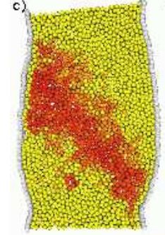
Framework 1: Particle systems

Outline

1   Framework 1: Particle systems
      Scaling Limits
      From discrete to continuous: the SPDE limit

2   Framework 2: Lattice Differential Equations
      Traveling waves in the PDE model
      Lattice models
      Influence of stochastic noise

    Carina Geldhauser (Lund)                      Discrete SPDEs   FAU-DCN 2021   4 / 23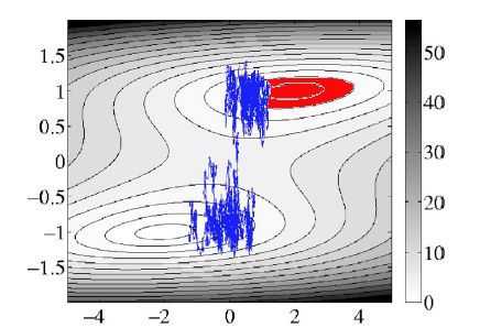
Framework 1: Particle systems
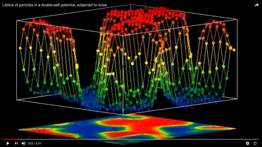
What is an interacting particle system?
model complex phenomena with large number of components (spins,
bacteria...)
each particle Xi moves according to a rule (e.g. differential equation)
add stochastic term to the movement rule (e.g. ODE) to
model microscopic influences or unresolved degrees of freedom
A particle Xi is a function of time (and
ω), labelled by i = 1 . . . N
Xi : [0, T ] × Ω → R
(t, ω) 7→ Xi (t, ω)
| {z }
position of Xi
Figure: Lattice of interacting particles, by Nils Berglund
Video (Nils Berglund): 128 harmonically coupled Xi , subj. t. white noise
Carina Geldhauser (Lund) Discrete SPDEs FAU-DCN 2021 5 / 23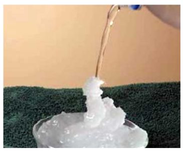
Framework 1: Particle systems

Noise-induced metastability

    rare, abrupt transition from one (meta)stable state to another
    Questions: expected transition time? most likely transition path?

    Figure: energy level of conformations of cyclohexane       Figure: transition path: Adams & Vanden-Eijnden,
                                                               adapted by C.G.

  Carina Geldhauser (Lund)                         Discrete SPDEs                             FAU-DCN 2021        6 / 23
Framework 1: Particle systems
Local behaviour: symmetric bistable diffusion
√
dX (t) = 0
|{z} − V 0 (X (t))dt + 2σdB(t)
no interaction
movement of one particle X under local drift term −V 0 (u) = u − u 3
local dynamics tends to push the particle towards one of the two
stable positions ±1
noise adds small perturbation
4
3.5
3
2.5
2
1.5
1
0.5
0
−2 −1.5 −1 −0.5 0 0.5 1 1.5 2
1 4 1 2
V (u) = 4
u − 2
u Simulation by F. Barret
Carina Geldhauser (Lund) Discrete SPDEs FAU-DCN 2021 7 / 23Framework 1: Particle systems
Nearest-neighbour model
Setting: N particles Xi (t) on a lattice Λ = Z/NZ move according to
γh N i √
dXi (t) = Xi+1 (t) − 2XiN (t) + Xi−1
N
(t) dt−V 0 (Xi (t))dt + 2σd B
e i (t)
2
(SDE)
nearest-neighbour interaction, strength γ > 0 sufficiently strong to
allow synchronization
nonlinear local drift term: −V 0 (x ) = x − x 3 , B
e i indep. BM
Scaling limit
choose noise strength appropriately strong, perform diffusive rescaling
Result: solutions to the system (SDE) converge as N → ∞ to
solutions to the Stochastic Allen Cahn equation
Funaki, Gyöngy, Millet, Berglund, Gentz, Fernandez, Barret, Bovier, Meleard
Carina Geldhauser (Lund) Discrete SPDEs FAU-DCN 2021 8 / 23Framework 1: Particle systems Scaling Limits
From particles to (S)PDEs
Situation: Often particles = molecules, atoms .... # particles/mol ≈ 1023
Difficult to study a huge system of differential equations!
Goal: Want to find global or effective behaviour of the particle system
Strategy: Zoom out and let particle distance h → 0 (“Rescaling”)
Several scaling limits are used in statistical physics. 2 categories:
macroscopic limits
“effective” behaviour of the system, noise disappears as h → 0
example: hydrodynamic limit (à la Kipnis-Landim)
often: “speed up time” by a factor N 2 = 1/h2
mesoscopic limits (SPDE limits)
fluctuation is still present in the limit equation
example: SPDE limit
often “speed up time” by a factor N = 1/h
Carina Geldhauser (Lund) Discrete SPDEs FAU-DCN 2021 9 / 23Framework 1: Particle systems Scaling Limits
∗ Details on diffusive rescaling
1
Rescale Λ = Z/NZ by h = N uniform grid Th = {0, h, . . . , Nh}
Rescale the coupling constant γ by h−1 and V by h.
Accelerate time by a factor h1 , set Xe N (t) = X (t/h)
get a different sequence of indep. BM, call them Bi (t)
get extra h−1 for the interaction, the scaling h on V cancels out
Get rescaled system of SDEs for i ∈ Th
s
R
γ X 2σ
dui (t) = 3 2 JR (j) (ui+j (t) − ui (t)) dt − V 0 (ui (t))dt + dBi (t)
R h j=−R h
e N (t) ≡ ui (t) function of nodal values at the node i,
Notation: X i
h
u (t) = (u1 (t), . . . uN (t)) piecewise linear function on [0, 1].
Carina Geldhauser (Lund) Discrete SPDEs FAU-DCN 2021 10 / 23Framework 1: Particle systems From discrete to continuous: the SPDE limit
Types of interactions
N (t) − 2X N (t) + X N (t)
Nearest-neighbor-interaction: Xi+1 i i−1
0 i −R i −j i −2 i −1 i i +1 i +2 i +j i +R N
Long-range interaction: all particles Xj withdistance up to R to Xi
interact with strength JR (j) γ R N N
j=−R JR (j) Xi+j (t) − Xi (t)
P
J(-R) J(R)
0 i −R i −j i −2 i −1 i i +1 i +2 i +j i +R N
Our question: what happens if we take the simultaneous limit N → ∞
and R → ∞ in the long-range interaction system?
Carina Geldhauser (Lund) Discrete SPDEs FAU-DCN 2021 11 / 23Framework 1: Particle systems From discrete to continuous: the SPDE limit
Possible limit SPDEs
R
1 X
Denote formally Au := lim JR (j) (ui+j − ui ) .
h→0 R 3 h2
j=−R
What can be said about the limit equation
√
∂t u = γAu − V 0 (u) + 2σξ in T × R+ ? (SPDE)
For finite R and reasonable choices of JR (j), the limit operator A is (a
multiple of) the Laplacian ⇒ solutions to (SPDE) are 2α-Hölder in
1
space and α-Hölder in time for every α ∈ 0, 4 .
For R = h1 , the limit operator is given by A = J ∗ u
mean-field interaction, solutions only as regular as the noise
solutions to (SPDE) are distributions, u 3 is not defined
Our result: (SPDE) is well-defined up to R ∼ N ζ with ζ < 1/2.
Carina Geldhauser (Lund) Discrete SPDEs FAU-DCN 2021 12 / 23Framework 1: Particle systems From discrete to continuous: the SPDE limit
∗ Behaviour of the interaction term or: why ζ < 21 ?
Let λhk be the eigenvalues of γAhR ui = R 3γh2 RR
j=−R JR (j) (ui+j (t) − ui (t))
P
with periodic boundary conditions, satisfying x 2 J(x )dx = 1.
Proposition (Convergence of the discrete semigroup)
P1/h −tλhk h
Let gth (x , y ) = k=1 e vk (x )vkh (y ) and gt (x , y ) the heat semigroup.
Then, ∀ t0 > 0 ∃ c(γ, t0 ) such that for all (t, x , y ) ∈ [t0 , ∞) × [0, 1]2
|gth (x , y ) − gt (x , y )| ≤ c(γ, t0 )h2−2ζ .
Ingredients of the proof: Derive higher moment estimate
R −3 JR (j)j 4 = o(h−2ζ ) via the bound
P
1/h ζ−1
hX
X −1 1
λhk . + o(h1−2ζ )
k=1 k=1
k2
1
(which gives ζ < 2 ), and use this to prove |λk − λhk | . h2−2ζ .
Carina Geldhauser (Lund) Discrete SPDEs FAU-DCN 2021 13 / 23Framework 1: Particle systems From discrete to continuous: the SPDE limit
Results (informal summary)
More involved interactions
the scaling limit of the system with long-range interaction
PR 1
j=−R JR (j) (ui+j (t) − ui (t)) mit R . N 2 und JR (j) ≈ 1 is the
stochastic Allen-Cahn equation [Bovier, G. MPRF’17]
the transition times of short-range and long-range system are
comparable in the large N limit [MPRF’17]
Nonlocal interactions need polynomial decay in the interaction
strength (coefficients JR (j)), then they converge to ∆s , s ∈ ( 12 , 1)
Wellposedness of the SPDE limit
d = 1 proof by classical semigroup or variational techniques
d > 1 depends on the noise. For “regular” noise as in d = 1, for
additive space-time white noise by renormalization [DaPrato,
Debussche ’02], [Hairer ’13], [Gubinelli, Imkeller, Perkowski ’13]
Carina Geldhauser (Lund) Discrete SPDEs FAU-DCN 2021 14 / 23Framework 2: Lattice Differential Equations
Outline
1 Framework 1: Particle systems
Scaling Limits
From discrete to continuous: the SPDE limit
2 Framework 2: Lattice Differential Equations
Traveling waves in the PDE model
Lattice models
Influence of stochastic noise
Carina Geldhauser (Lund) Discrete SPDEs FAU-DCN 2021 14 / 23Framework 2: Lattice Differential Equations Traveling waves in the PDE model
Traveling waves in reaction-diffusion equations
Nagumo / Schlögl equation
For u(x , t) : R × R+ → R, consider
∂t u = ∆u − u(1 − u)(u − a)
with parameter a ∈ R
We observe:
For each a ∈ (0, 12 ), there exists a travelling front solution v (η) ≥ 0
with v (−∞) = 0 and v (+∞) = 1, v 0 (η) > 0.
Both the waves v (η) and their derivatives (∂η v )(η) decay
exponentially to their asymptotic limits as η → ±∞.
The wave speed s(a) < 0 is unique.
Carina Geldhauser (Lund) Discrete SPDEs FAU-DCN 2021 15 / 23Framework 2: Lattice Differential Equations Traveling waves in the PDE model
Why a lattice model?
electric signal jumps between gaps in myeline coating of nerve fibre
Model signal propagation by a Lattice Differential Equation (LDE):
solution ui at node i = electric potential at i-th myeline gap
Carina Geldhauser (Lund) Discrete SPDEs FAU-DCN 2021 16 / 23Framework 2: Lattice Differential Equations Traveling waves in the PDE model
Semidiscrete reaction-diffusion equations
Example: discrete-in-space Nagumo equation on lattice Z
1
∂t ui = (ui+1 + ui−1 − 2ui ) + (1 − ui2 )(ui − a)
h2
a ∈ [−1, 1] “excitable regime”
traveling waves
u(x , t) = u TW (x − ct)
with speed c
Figure: asymmetric reaction term
f (u) := (u − 1)(u + 1)(u − a)
“Pinning” phenomenon: if grid size h too large (depending on a),
stationary solutions, maybe non-unique, speed c = 0. [Keener], others
Carina Geldhauser (Lund) Discrete SPDEs FAU-DCN 2021 17 / 23Framework 2: Lattice Differential Equations Lattice models
A stochastic lattice model
(Ω, F, (Ft )t , P) filtered probability space, noise is Q-Wiener on L2 (D) with
covariance operator Q pos. semi-definite, symmetric, ∞ k=1 µk < ∞
P
Space-discrete model: Stochastic Nagumo equation on a 1D lattice Z
R
X
u̇i (t) = ν J(j) (ui+j (t) − ui (t)) + f (ui (t)) + g(ui (t))Bi (t)
| {z } | {z }
j=−R
| {z } wave-type solutions unresolved dof
synapse interaction
Here, g : R → R comes from a multiplicative noise term, defined via
(G(u)χ) (x ) := g(u(x ))χ(x ) for u, χ ∈ L2 (D) G(u) : L2 (D) → H,
Lipschitz continuous, linear growth conditions.
Simulation 1: Pulse in FitzHughNagumo eq., N=400, by Christian Kühn
Simulation 2: Pulse in FitzHughNagumo eq., N=200, by Christian Kühn
Carina Geldhauser (Lund) Discrete SPDEs FAU-DCN 2021 18 / 23Framework 2: Lattice Differential Equations Influence of stochastic noise
Result: stability of the wave in the semidiscrete model
Informal idea:
Assume that the noise acts on the transition part of the wave, i.e.
g(0) = g(1) = 0.
Compare our lattice solution with a deterministic reference wave
Theorem (Stability of traveling waves (G. & Kuehn ’20))
Under suitable parameter conditions, and if the covariance of the noise is
sufficiently small, the discrete-stochastic variant of the Nagumo equation
has solutions u h , for which holds
" #
h TW
P sup ku (t) − v (t)kL2 (R) > δ ≤ ε
t∈[0,T ]
for sufficiently small h and T < t∗ .
Carina Geldhauser (Lund) Discrete SPDEs FAU-DCN 2021 19 / 23Framework 2: Lattice Differential Equations Influence of stochastic noise
Remarks
The probability that t∗ is infinite depends on the initial error
kv0 − v TW (0)k and on the covariance operator of the noise term.
Breakdown of the wave (i.e. t∗ finite)
depends on the initial error kv0 − v TW (0)k and on the covariance
The smaller the covariance operator of the noise term kQk2HS , the
smaller the probability for t∗ being finite.
zero covariance does not imply that the noise strength is zero, but
just that it is constant, and so it affects the solution only by a shift of
c · t, which does not destroy the traveling wave property.
Restrictions
The result covers only the case where there is no pinning, i.e the grid
is fine enough, due to the need of a deterministic reference wave
For non-trace-class noise, need other techniques
Carina Geldhauser (Lund) Discrete SPDEs FAU-DCN 2021 20 / 23Framework 2: Lattice Differential Equations Influence of stochastic noise
Overview: front propagation in 1D, discretization, noise
Influence of discretization (on the deterministic equation)
Continuous equation: Existence of traveling wave solutions
u(x , t) = u(x − ct) with limξ→±∞ u(ξ) = ±1 . Speed c
Semidiscrete equation: solution profile might change shape, be
step-like (”lurching” in the motion of the interface), slow down or fail
to propagate (space-discrete), speed up (time-discrete)
Fully discrete equation: nonuniqueness of the pair wave speed -
solution profile
Influence of noise on the space-discrete model
Stability of traveling waves −→ TODAY
changes to speed and form of traveling wave solutions? −→ ongoing
Carina Geldhauser (Lund) Discrete SPDEs FAU-DCN 2021 21 / 23Framework 2: Lattice Differential Equations Influence of stochastic noise
Ongoing work: speed close to pinning
Maths observation: “Pinning” phenomenon: if grid size h too large
(depending on a), stationary solutions, maybe non-unique, speed c = 0.
[Keener ’87], many many others
Simulations done in a deterministic lattice model:
Figure: Shape (left) and speed (right) of deterministic traveling wave φ. Autor: H.J. Hupkes
Ongoing work: Investigate speed of the wave as h approaches the critical
value h(a), with S. Tikhomirov (St. Petersburg) and H.J. Hupkes (Leiden)
Carina Geldhauser (Lund) Discrete SPDEs FAU-DCN 2021 22 / 23Framework 2: Lattice Differential Equations Influence of stochastic noise References A. Bovier and C. Geldhauser. The scaling limit of a particle system with long-range interaction. Markov Proc. Rel. Fields 2017. C. Geldhauser and Ch. Kuehn. Travelling waves for discrete stochastic bistable equations. https://arxiv.org/abs/2003.03682 2020. N. Berglund and B. Gentz. Sharp estimates for metastable lifetimes in parabolic SPDEs: Kramers’ law and beyond. Electron. J. Probab., 2013. W. Stannat Stability of travelling waves in stochastic Nagumo equations. https://arxiv.org/abs/1301.6378 2013. Carina Geldhauser (Lund) Discrete SPDEs FAU-DCN 2021 23 / 23
You can also read