SAFARI fact sheet - The Spica Mission
←
→
Page content transcription
If your browser does not render page correctly, please read the page content below
SAFARI fact sheet
1 Introduction
The purpose of this note is to explain and provide guidance on how-to-use the SAFARI fact
sheet version 1.0. The term “fact sheet” is itself misleading, there are no “facts”’ in the
sheet just current best guesses. The sensitivities noted in the sheet are based on a very
simplistic model of SAFARI with no spectral or spatial variation across a sub-band. The fact-
sheet can be used to estimate the time to execute observation programs but with
uncertainty. It should not be used to “optimize” a science program.
Bear in mind that any estimate will be without calibrations and other overheads.
2 SAFARI bands and band – properties
SAFARI will use 4 spectral bands covering the spectral range from 34 to 230 µm. Three
significant band parameters are listed in the table 1. The FWHM parameter identifies the
SAFARI beam at the band center.
Table 1: Parameters of SAFARI wavebands
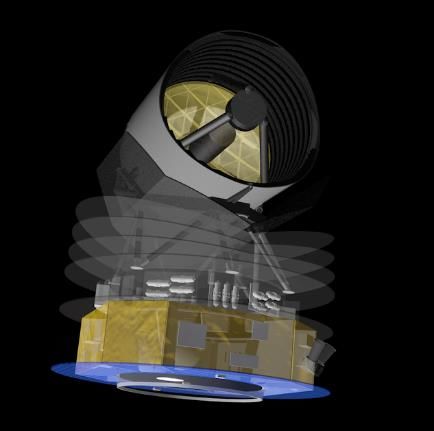
3 Instrument and Noise Model
The current SAFARI sensitivity model is built up from best guesses for what the actual
telescope and instrument will be.
• SAFARI sensitivity model ingredients
• Telescope: M1 2.5 m, M2 60 cm à Aeff 4.6 m2
• Component efficiencies, aperture, horn, etc. : total η = 0.22
• All optics elements – at 4K, 1.7K, 0.3K and 0.05K
• Transmission T of grating, mirrors, and filters: à Toptics ~ 0.24
• Emission ε = 1 – T
• Power from Zodiacal light – JWST/MIRI model
• Two blackbody model: 5500K/ε=3.5×10-14 and 270K /ε=3.6×10-8
• f(pole)~0.9, f(ecliptic)~8 à model uses f=2.5
• Power from zodiacal light, source and optics/telescope/baffle transmitted to
detector à photon NEPphot
• Power from astronomical source (see Figure 1)
•   Astronomical source is assumed spatially unresolved.
       •   Detector noise as per requirement NEPdet = 2×10-19 W/√Hz

              σlim • √(NEPdet2 + NEPphot2 )
       ΔF = --------------------------------------- W/m2
              Aeff • η • Toptics • √(2 • tobs)

5 σ detection à σlim = 5: Signal /Noise ratio of 5
σ à noise in W/m2
1 hr observations à tobs = 3600 sec

4 Time Estimation for point source spectroscopy
The sensitivity table results from the instrument noise model in the section above which
provides the estimated noise per detector. In the noise model, the sensitivity within a sub-
band is only slightly wavelength dependent and therefore considered constant throughout a
sub-band.

For the sensitivities listed in Table 2, a detection sequence is assumed where an off position
has been subtracted which increases the limiting flux per detector by about 20%.

Table 2: Limiting flux and flux density for point sources

Time estimation for SAFARI is simple:
          • 1 hour integration can observe: ~ 6-8 x 10-20 W/m2 at 5σ
          • Signal (5 x noise level) after time T hours: ~ 7 x 10-20 / √T W/m2
          • For FTS operation use ~ 1.4 x 10⁻¹⁹ W/m2 (single pol. à factor 2 loss)
              with 3 scans as minimum time à 9 minutes
          • For mapping – use same algorithm per pixel i.e., raster mapping.
          • Not yet addressed – scan maps, optimized strategy for FTS maps

The “LR” mode in the factsheet refers to the sky signal passing thing through the grating.
Whereas the “HR” refers to observing the sky with the Martin-Puplet interferometer
inserted before the grating.
4.1 Grating observation of point source
               The calculations assume a spatial unresolved point source with spectrally unresolved lines.
               The fact sheet numbers give the 5 sigma flux that a detector can measure in one hour. That

I Fact Sheet
               is to say, the signal-to-noise of the resulting measurement is 5. The noise is assumed to be
               white.

               SPICA       Mission
               The grating should produce a spectral resolution of about 300 at the band center (nc/dnc).
               •In ESA/JAXA
                   the current collaboration
                                configuration, this spectrum will be sampled twice within each resolution
               •element.
                   Telescope effective area 4.6 m2
               • Primary mirror temperature 8K
               •TheGoal
                     flux mission
                          density inlifetime  – 5the
                                      Table 2 for years
                                                     LR mode depends on the wavelength since the resolution
        LLW
               is assumed constant over the waveband (as opposed to the HR mode, see below)
        185

               4.2   FTS
                System   observation
                       performance       of point source
                                   v.s. target
 3   140-230
               The
                fluxhigh   frequency
                     density,  relative tomode
                                           the of SAFARI is achieved with a Martin-Puplet Interferometer. The
                background limited case
        19”    FTS  cansensitivity
                • The     only make     use of
                                    decrease     one polarization. This means that the limiting source flux is ~ 2
                                              is due
               higher   than
                   to the     the low-resolution
                          increased   photon noise    mode.
                  from the target source                                LR mode
                • Data given up to the                                HR mode
                  instrument
               Theeach
                    spectral  saturation limits for
                              resolution in high resolution mode is determined entirely by the maximum
        8.2             band (31, 51 and 87 Jy
               optical  path
                  for the SW,displacement
                               MW and LW bands  (OPD) of the interferometer. For SAFARI, the result is a constant
        1.44      respectively.
               frequency resolution of 0.749 GHz. This is reflected in Table 2 as a relatively constant flux
         15
               density limit across all wavebands. The resolution as a function of wavelength is shown in
               Figure 1.
         19

                 R                                              SAFARI/HR resolution as
                10000                                            function of wavelength
         23

         4.1       8000

         51        6000
         67
                   4000

                   2000
        239
 y    10 mJy          0
                                                                                              λ
√Hz                       30        80          130          180          230         280 (µm)
 f 1 arcmin2
               Figure 1: Spectral resolution of the FTS.
                                                      SAFARI GS Factsheet V1.0 – 30th September 2016

               5     Band centers
               All sensitivities and band parameters are appropriate for the band centers. There will be
               some changes near the edges of the bands i.e. sensitivity, resolution of grating and beam
               FWHM. For the purpose of rough ideas about length of projects, the band center values are
               the most appropriate.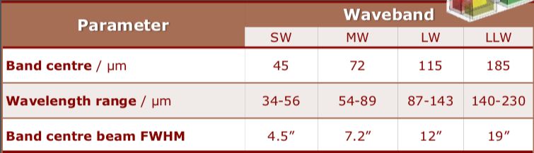
6 Source brightness and saturation
SAFARI grating is detector noise limited but close to background limited. There are lines-of-
sight where the background photons are contributing the greatest fraction of the noise.
That will be true in the Ecliptic and Galactic Plane. The noise values below assume a mid-
latitude ecliptic elevation (~30% of maximum zodiacal contamination) and away from the
Galactic Plane. The zodiacal model is that used by MIRI for JWST.

The observed source will add to the photon noise to achieved noise level. Figure 2 shows
the fractional added noise level given the strength of the astronomical source up to the
saturation limit where each curve stops. Data given up to the instrument flux density
saturation limits for each band (31, 51, 87 and 131 Jy for the SW, MW, LW and VLW bands
respectively, shown in the figure as colored circles). This correction must be taken into
account when observing a week line on top of a bright continuum.

For example, the expected noise in the SW band observing a source of 200 mJy is about 2
times the most sensitive case i.e., observing to the same signal-to-noise level will take 4
times as long. A 5σ detection of 0.31 mJy on a continuum-free source takes 1 hr. With a
200 mJy continuum, detecting 0.31 mJy above the continuum (total 200.31 mJy) takes 4 hrs.

Figure 2: Sensitivity degradation factor based on source flux density. Solid lines and dashed
lines are for the low resolution grating and high resolution FTS respectively. Colors indicate
which wavelength band the curve applies. The solid circles indicate saturation limits.

7 Mapping modes:
The fact sheet also estimates the time to map using SAFARI either in low resolution mode
(LR) or high resolution (HR) (Table 3). In this calculation, only raster mapping is considered.
For each SAFARI band (SW, MW, LW and VLW) the table lists the limiting flux (at 5σ) per
map position that would be achieve for a Nyquist sampled map of 1 arcmin2. Note that the
Nyquist sampled map is achieved for the central wavelength of each band.

Unlike the point source calculation, the map noise estimate does not account for
subtracting a “zero” level.

As with the point source mode, the observed noise towards a position will increase with the
brightness of the background source (see Figure 2).

Table 3: Limiting flux and flux density for mapping

8 Photometric Mapping
The fact sheet also list limits for a photometric mapping mode where all detectors within a
waveband are averaged. As can be seen in table 4, such a mode will quickly run into the
source confusion limit in the longest waveband.

All mapping mode limits are 1 hour integration of a 1 armin2 area.

Table 4: Sensitivity and confusion limits
You can also read