Super-Resolution of Sentinel-2 Images: Learning a Globally Applicable Deep Neural Network
←
→
Page content transcription
If your browser does not render page correctly, please read the page content below
Super-Resolution of Sentinel-2 Images: Learning a Globally Applicable Deep Neural
Network
Charis Lanarasa,∗, José Bioucas-Diasb , Silvano Galliania , Emmanuel Baltsaviasa , Konrad Schindlera
a Photogrammetry and Remote Sensing, ETH Zurich, Zurich, Switzerland
b Instituto de Telecomunicações, Instituto Superior Técnico, Universidade de Lisboa, Portugal
Abstract
The Sentinel-2 satellite mission delivers multi-spectral imagery with 13 spectral bands, acquired at three different spatial resolu-
tions. The aim of this research is to super-resolve the lower-resolution (20 m and 60 m Ground Sampling Distance – GSD) bands to
arXiv:1803.04271v1 [cs.CV] 12 Mar 2018
10 m GSD, so as to obtain a complete data cube at the maximal sensor resolution. We employ a state-of-the-art convolutional neural
network (CNN) to perform end-to-end upsampling, which is trained with data at lower resolution, i.e., from 40→20 m, respectively
360→60 m GSD. In this way, one has access to a virtually infinite amount of training data, by downsampling real Sentinel-2 images.
We use data sampled globally over a wide range of geographical locations, to obtain a network that generalises across different cli-
mate zones and land-cover types, and can super-resolve arbitrary Sentinel-2 images without the need of retraining. In quantitative
evaluations (at lower scale, where ground truth is available), our network outperforms the best competing approach by almost 50%
in RMSE, while better preserving the spectral characteristics. It also delivers visually convincing results at the full 10 m GSD.
Keywords: Sentinel-2; super-resolution; sharpening of bands; convolutional neural network; deep learning
1. Introduction Sentinel-2 (S2) consists of two identical satellites, 2A and
2B, which use identical sensors and fly on the same orbit with
Several widely used satellite imagers record multiple spectral
a phase difference of 180 degrees, decreasing thus the repeat
bands with different spatial resolutions. Such instruments have
and revisit periods. The sensor acquires 13 spectral bands with
the considerable advantage that the different spectral bands
10 m, 20 m and 60 m resolution, with high spatial, spectral, ra-
are recorded (quasi-)simultaneously, thus with similar illumi-
diometric and temporal resolution, compared to other, similar
nation and atmospheric conditions, and without multi-temporal
instruments. More details on the S2 mission and data are given
changes. Furthermore, the viewing directions are (almost)
in Section 3. Despite its recency, S2 data have been already ex-
the same for all bands, and the co-registration between bands
tensively used. Beyond conventional thematic and land-cover
is typically very precise. Examples of such multi-spectral,
mapping, the sensor characteristics also favour applications like
multi-resolution sensors include: MODIS, VIIRS, ASTER,
hydrology and water resource management, or monitoring of
Worlview-3 and Sentinel-2. The resolutions between the spec-
dynamically changing geophysical variables.
tral bands of any single instrument typically differ by a factor
E.g., Mura et al. (2018) exploit S2 to predict growing stock
of about 2 to 6. Reasons for recording at varying spatial resolu-
volume in forest ecosystems. Castillo et al. (2017) compute the
tion include: storage and transmission bandwidth restrictions,
Leaf Area Index (LAI) as a proxy for above-ground biomass of
improved signal-to-noise ratio (SNR) in some bands through
mangrove forests in the Philippines. Paul et al. (2016) map the
larger pixels, and bands designed for specific purposes that
extent of glaciers, while Toming et al. (2016) map lake water
do not require high spatial resolution (e.g. atmospheric correc-
quality. Immitzer et al. (2016) have demonstrated the use of S2
tions). Still, it is often desired to have all bands available at the
data for crop and tree species classification, and Pesaresi et al.
highest spatial resolution, and the question arises whether it is
(2016) for detecting built-up areas. The quality, free availability
possible to computationally super-resolve the lower-resolution
and world-wide coverage make S2 an important tool for (cur-
bands, so as to support more detailed and accurate information
rent and) future earth observation, which motivates this work.
extraction. Such a high-quality super-resolution, beyond naive
Obviously, low-resolution images can be upsampled with
interpolation or pan-sharpening, is the topic of this paper. We
simple and fast, but naive methods like bilinear or bicubic inter-
focus specifically on super-resolution of Sentinel-2 images.
polation. However, such methods return blurry images with lit-
∗ Corresponding author tle additional information content. More “sophisticated” meth-
Email addresses: charis.lanaras@geod.baug.ethz.ch (Charis ods, including ours, attempt to do better and recover as much
Lanaras), bioucas@lx.it.pt (José Bioucas-Dias), as possible of the spatial detail, through a “smarter” upsam-
silvano.galliani@geod.baug.ethz.ch (Silvano Galliani),
emmanuel.baltsavias@geod.baug.ethz.ch (Emmanuel
pling that is informed by the available high-resolution bands.
Baltsavias), konrad.schindler@geod.baug.ethz.ch (Konrad Here, we propose a (deep) machine learning approach to multi-
Schindler) spectral super-resolution, using convolutional neural networks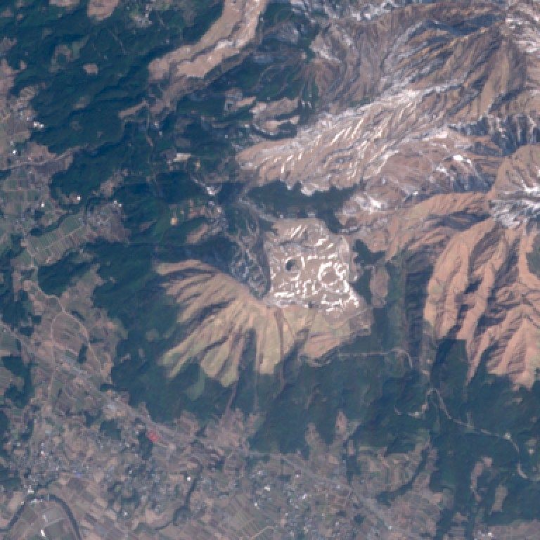
could be achieved, if a user focusing on a specific task and geo-
                                                                                graphic region retrains the proposed networks with images from
                                                                                that particular environment. In that case, one can start from our
                                                                                trained network and fine-tune the network weights with appro-
                                                                                priate training sites. However, our experiments show that even
                                                                                a single model, trained on a selected set of representative sites
                                                                                world-wide, achieves much better super-resolution than prior
                                                                                state-of-the-art methods for independent test sites, also sam-
                                                                                pled globally. That is, our network is not overfitted to a par-
                                                                                ticular context (as often the case with discriminative statistical
        10 m                     20 m                     60 m                  learning), but can be applied worldwide.
                                                                                   Extensive experimental tests at reduced scale (where S2
                                                                                ground truth is available) show that our single, globally ap-
                                                                                plicable network yields greatly improved super-resolution of
                                                                                all S2 bands to 10 m GSD. We compare our method to four
                                                                                other methods both quantitatively and qualitatively. Our ap-
                                                                                proach achieves almost 50% lower RMSE than the best compet-
     DSen2                                                                      ing methods, as well as > 5 dB higher signal-to-reconstruction-
 Super-Resolution                                                               error ratio and >30% improvement in spectral angle mapping.
                                                                                The performance difference is particularly pronounced for the
                                                                                Short-Wave Infrared (SWIR) bands and the 60 m ones, which
                                 10 m                    10 m                   are particularly challenging for super-resolution. For com-
Figure 1: Top: Input Sentinel-2 bands at 10 m, 20 m and 60 m GSD, Bottom:       pleteness, we also provide results for three “classical” pan-
Super-Resolved bands to 10 m GSD, with the proposed method (DSen2).             sharpening methods on the 20 m bands, which confirm that
                                                                                pan-sharpening cannot compete with true multi-band super-
                                                                                resolution methods, including ours. Importantly, we also train a
(CNNs). The goal is to surpass the current state-of-the-art in                  version of our network at half resolution (80→40 m) and eval-
terms of reconstruction accuracy, while at the same time to pre-                uate its performance on 40→20 m test data. While there is
serve the spectral information of the original bands. Moreover,                 of course some loss in performance, the CNN trained in this
the method shall be computationally efficient enough for large-                 way still performs significantly better than all other methods.
area practical use. We train two CNNs, one for super-resolving                  This supports our assertion that the mapping is to a large ex-
20 m bands to 10 m, and one for super-resolving 60 m bands                      tent scale-invariant and can be learned from training data at
to 10 m. Our method, termed DSen2, implicitly captures the                      reduced resolution – which is important for machine learning
statistics of all bands and their correlations, and jointly super-              approaches in general, beyond our specific implementation.
resolves the lower-resolution bands to 10 m GSD. See an ex-                        Summarising our contributions, we have developed a CNN-
ample in Figure 1. True to the statistical learning paradigm, we                based super-resolution algorithm optimised for (but conceptu-
learn an end-to-end-mapping from raw S2 imagery to super-                       ally not limited to) S2, with the following characteristics: (i)
resolved bands purely from the statistics over a large amount                   significantly higher accuracy of all super-resolved bands, (ii)
of image data. Our approach is based on one main assumption,                    better preservation of spectral characteristics, (iii) favourable
namely that the spectral correlation of the image texture is self-              computational speed when run on modern GPUs, (iv) global
similar over a (limited) range of scales. I.e., we postulate that               applicability for S2 data without retraining, according to our
upsampling from 20 m to 10 m GSD, by transferring high reso-                    (necessarily limited) tests, (v) generic end-to-end system that
lution (10 m) details across spectral bands, can be learned from                can, if desired, be retrained for specific geographical locations
ground truth images at 40 m and 20 m GSD; and similarly for                     and land-covers, simply by running additional training itera-
the 60 m to 10 m case. Under this assumption, creating train-                   tions, (vi) free, publicly available source code and pre-trained
ing data for supervised learning is simple and cheap: we only                   network weights, enabling out-of-the-box super-resolution of
need to synthetically downsample original S2 images by the de-                  S2 data.
sired factor, use the downsampled version as input to generate
original data as output.
                                                                                2. Related Work
   In this way, one gains access to large amounts of training
data, as required for deep learning: S2 data are available free                    Enhancing the spatial resolution of remotely sensed multi-
of charge, covering all continents, climate zones, biomes and                   resolution images has been addressed for various types of im-
land-cover types. Moreover, we assert that the high-capacity                    ages and sensors, including for example ASTER (Tonooka,
of modern deep neural networks is sufficient to encode a super-                 2005; Fasbender et al., 2008), MODIS (Trishchenko et al.,
resolution mapping which is valid across the globe. Fig. 2 and 3                2006; Sirguey et al., 2008), and VIIRS (Picaro et al., 2016).
show various land-cover types and geographical/climatic areas                   In the following, we differentiate three types of methods: pan-
used for training and testing. It is likely that even better results            sharpening per band, inverting an explicit imaging model, and
                                                                            2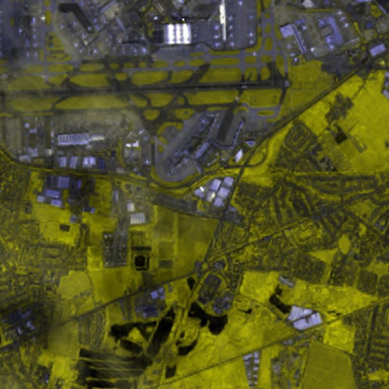
Figure 2: A selection of the images used for training and testing.

machine learning approaches. The first group increases the spa-             compared to naive nearest neighbor upsampling. Interestingly,
tial resolution independently for each target band, by blending             the classification results improved for most of the methods.
in information from a spectrally overlapping high-resolution                   The second group of methods attacks super-resolution as
band. It is therefore essentially equivalent to classical pan-              an inverse imaging problem under the variational, respectively
sharpening, applied separately to the spectral region around                Bayesian, inference frameworks. These model-based meth-
each high-resolution band. Such an approach relies on the as-               ods are conceptually appealing in that they put forward an ex-
sumption that for each relevant portion of the spectrum there               plicit observation model, which describes the assumed blurring,
is one high-resolution band (in classical pan-sharpening the                downsampling, and noise processes. As the inverse problem
“panchromatic” one), which overlaps, at least partially, with               is ill-posed by definition, they also add an explicit regulariser
the lower-resolution bands to be enhanced. That view leads                  (in Bayesian terms an “image prior”). The high-resolution
directly to the inverse problem of undoing the spatial blur from            image is then obtained by minimising the residual error w.r.t.
the panchromatic to the lower-resolution texture. A number of               the model (respectively, the negative log-likelihood of the pre-
computational tools have been applied ranging from straight-                dicted image) in a single optimisation for all bands simultane-
forward component substitution to multiresolution analysis,                 ously. Brodu (2017) introduced a method that separates band-
Bayesian inference and variational regularisation. For a few                dependent spectral information from information that is com-
representative examples we refer to (Choi et al., 2011), (Lee               mon across all bands, termed “geometry of scene elements”.
and Lee, 2010) and (Garzelli et al., 2008). A recent review and             The model then super-resolves the low-resolution bands such
comparison of pan-sharpening methods can be found in Vivone                 that they are consistent with those scene elements, while pre-
et al. (2015). The pan-sharpening strategy has also been ap-                serving their overall reflectance. Lanaras et al. (2017) adopt
plied directly to Sentinel-2, although the sensor does not meet             an observation model with per-band point spread functions that
the underlying assumptions: as opposed to a number of other                 account for convolutional blur, downsampling, and noise. The
earth observation satellites (e.g., Landsat 8) it does not have             regularisation consists of two parts, a dimensionality reduction
a panchromatic band that covers most of the sensor’s spec-                  that implies correlation between the bands, and thus lower in-
tral range. In a comparative study Vaiopoulos and Karantza-                 trinsic dimension of the signal; and a spatially varying, contrast-
los (2016) evaluate 21 pan-sharpening algorithms to enhance                 dependent penalisation of the (quadratic) gradients, which is
the 20 m visible and near infrared (VNIR) and short wave in-                learned from the 10 m bands. SMUSH, introduced in Paris et al.
frared (SWIR) bands of Sentinel-2, using heuristics to select               (2017), adopts an observation model similar to Lanaras et al.
or synthesise the “panchromatic” input from the (in most cases              (2017), but employs a different, patch-based regularisation that
non-overlapping) 10 m bands. Wang et al. (2016) report some                 promotes self-similarity of the images. The method proceeds
of the best results in the literature for their ATPRK (Area-                hierarchically, first sharpening the 20 m bands, then the coarse
To-Point Regression Kriging) method, which includes a simi-                 60 m ones.
lar band selection, performs regression analysis between bands                 The third group of super-resolution methods casts the pre-
at low resolution, and applies the estimated regression coeffi-             diction of the high-resolution data cube as a supervised machine
cients to the high-resolution input, with appropriate normalisa-            learning problem. In contrast to the two previous groups, the re-
tion. Park et al. (2017) propose a number of modifications to               lation between lower-resolution input to higher-resolution out-
optimise the band selection and synthesis, which is then used               put is not explicitly specified, but learned from example data.
for pan-sharpening with component substitution and multireso-               Learning methods (and in particular, deep neural networks) can
lution analysis. Du et al. (2016), having in mind the monitoring            thus capture much more complex and general relations, but in
of open water bodies, have tested four popular pan-sharpening               turn require massive amounts of training data, and large com-
methods to sharpen the B11 SWIR band of S2, in order to com-                putational resources to solve the underlying, extremely high-
pute a high-resolution the normalized differential water index              dimensional and complex optimisation. We note that the meth-
(NDWI). Further in this direction, Gasparovic and Jogun (2018)              ods described in the following were designed with the classic
used five different pan-sharpening methods to enhance the res-              pan-sharpening problem in mind. Due to the generic nature of
olution of the 20 m bands. Their goal was to investigate the                end-to-end machine learning, this does not constitute a concep-
effect of the sharpened images on a land-cover classification               tual problem: in principle, they could be retrained with different
                                                                        3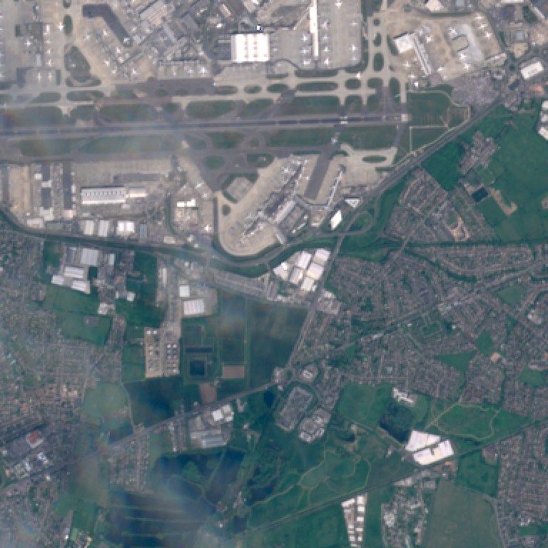
input and output dimensions. Obviously, their current weights
are not suitable for Sentinel-2 upsampling. To the best of our
knowledge, we are the first to apply deep learning to that prob-
lem. Masi et al. (2016) adapt a comparatively shallow three-
layer CNN architecture originally designed for single-image                           Polar and subpolar zone
                                                                                      Temperate zone
(blind) super-resolution. They train pan-sharpening networks                          Subtropical zone
                                                                                      Tropical zone
for Ikonos, GeoEye-1 and WorldWiew-2. More recently, Yang                             Training sites
                                                                                      Testing sites
et al. (2017) introduced PanNet, based on the high-performance
ResNet architecture (He et al., 2016). PanNet starts by upsam-
pling the low-resolution inputs with naive interpolation. The
actual network is fed with high-pass filtered versions of the
raw inputs and learns a correction that is added to the naively
upsampled images.1 PanNet was trained for Worldview-2,                             Figure 3: Locations of Sentinel-2 tiles used for training and testing. Image
                                                                                   source: meteoblue.com
Worldview-3, and Ikonos. Both described pan-sharpening net-
works are trained with relatively small amounts of data, pre-
sumably because of the high data cost. In this context, we point                   absolute radiometric uncertainty (except B10)  27% margin.
acteristics like for instance spectral response functions. Rather,                    Clerc and MPC Team (2018) report on further aspects of S2
the sensor properties are implicit in the training data.                           data quality. The mean pairwise co-registration errors between
                                                                                   spectral bands are 0.14–0.21 pixels (at the lower of the two res-
                                                                                   olutions) for S2A and 0.07–0.18 pixels for S2B, 99.7% confi-
3. Input data
                                                                                   dence. This parameter is important for our application: good
   We use data from the ESA/Copernicus satellites Sentinel 2A                      band-to-band co-registration is important for super-resolution,
and 2B2 . They were launched on June 23, 2015 and March 7,                         and S2 errors are low enough to ignore them and proceed with-
2017, respectively, with a design lifetime of 7.25 years, poten-                   out correcting band-to-band offsets. Moreover, data quality is
tially extendible up to 5 additional years. The two satellites are                 very similar for Sentinel-2A and 2B, so that no separate treat-
identical and have the same sun-synchronous, quasi-circular,                       ment is required. B10 (in an atmospheric absorption window,
near-polar, low-earth orbit with a phase difference of 180 de-                     included for cirrus clouds detection) has comparatively poor
grees. This allows the reduction of the repeat (and revisit) pe-                   radiometric quality and exhibits across-track striping artifacts,
riods from 10 to 5 days at the equator. The satellites system-                     and is excluded from many aspects of quality control. For that
atically cover all land masses except Antarctica, including all                    reason we also exclude it.
major and some smaller islands. The main sensor on the satel-                         Potential sensor issues that could impair super-resolution
lites is a multispectral imager with 13 bands. Their spectral                      would mainly be band-to-band misregistration (which is very
characteristics and GSDs are shown in Table 1. Applications of                     low for S2), radiometric or geometric misalignments within a
the 10 m and 20 m bands include: general land-cover mapping,                       band (which do not seem to occur), and moving objects such
agriculture, forestry, mapping of biophysical variables (for in-                   as airplanes (which are very rare). The data thus fulfills the
stance, leaf chlorophyll content, leaf water content, leaf area                    preconditions for super-resolution, and we did not notice any
index), monitoring of coastal and inland waters, and risk and                      effects in our results that we attribute to sensor anomalies.
disaster mapping. The three bands with 60 m GSD are intended                          S2 data can be downloaded from the Copernicus Services
mainly for water vapour, aerosol corrections and cirrus clouds                     Data Hub, free of charge. The data comes in tiles (gran-
estimation. In actual fact they are captured at 20 m GSD and                       ules) of 110×110 km2 (≈800MB per tile). For processing, we
are downsampled in software to 60 m, thus increasing the SNR.                      use the Level-1C top-of-atmosphere (TOA) reflectance prod-
The first 10 bands cover the VNIR spectrum and are acquired                        uct, which includes the usual radiometric and geometric cor-
by a CMOS detector for two bands (B3 and B4) with 2-line                           rections. The images are geocoded and orthorectified using the
TDI (time delay and integration) for better signal quality. The                    90m DEM grid (PlanetDEM3 ) with a height (LE95) and plani-
last 3 bands cover the SWIR spectrum and are acquired by pas-                      metric (CE95) accuracy of 14 m and 10 m, respectively. We
sively cooled HgCdTe detectors. Bands B11 and B12 also have                        note that a refinement step for the Level-1C processing chain
staggered-row, 2-line TDI. The swath width is 290 km. Inten-                       is planned, which shall bring the geocoding accuracy between
sities are quantised to 12 bit and compressed by a factor ≈2.9                     different passes to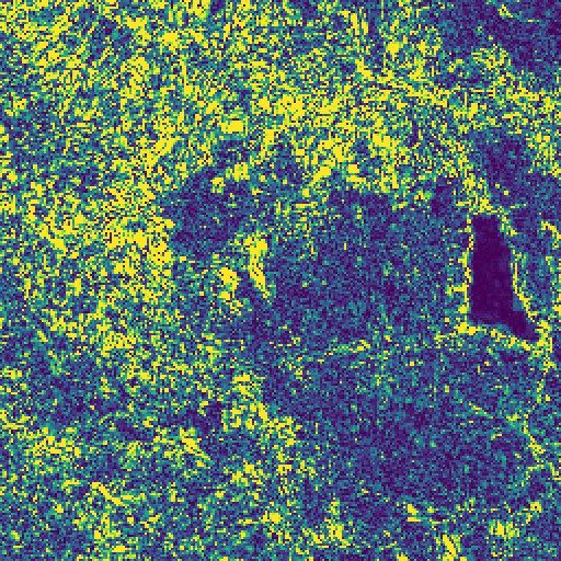
Table 1: The 13 Sentinel-2 bands.
           Band                       B1     B2    B3     B4      B5      B6      B7       B8        B8a   B9        B10   B11     B12
           Center wavelength [nm]    443    490   560     665    705     740     783       842       865   945      1380   1610   2190
           Bandwidth [nm]             20     65    35      30     15      15      20       115        20    20        30     90    180
           Spatial Resolution [m]     60     10    10      10     20      20      20        10        20    60        60     20     20

zones, land-cover and biome types. Using this wide variety of                               filter               filter    downsampling
scenes, we aim to train a globally applicable super-resolution                            Gaussian           Boxcar
network that can be applied to any S2 scene.
                                                                          S2 band                                                         training
                                                                                                                                          data
4. Method
                                                                         Figure 4: The downsampling process used for simulating the data for training
   We adopt a deep learning approach to Sentinel-2 super-                and testing.
resolution. The rationale is that the relation between the multi-
resolution input and a uniform, high-resolution output data cube
is a complex mixture of correlations across many (perhaps all)
spectral bands, over a potentially large spatial context, respec-        to learn how to transfer high frequency details from existing
tively texture neighbourhood. It is thus not obvious how to de-          high-resolution bands. The literature on self-similarity in im-
sign a suitable prior (regulariser) for the mapping. On the con-         age analysis supports such an assumption (e.g., Shechtman and
trary, the underlying statistics can be assumed to be the same           Irani, 2007; Glasner et al., 2009), at least over a certain scale
across different Sentinel-2 images. We therefore use a CNN to            range. We emphasise that for our case, the assumption must
directly learn it from data. In other words, the network serves as       hold only over a limited range up to 6× resolution differences,
a big regression engine from raw multi-resolution input patches          i.e., less than one order of magnitude. In this way, virtually
to high-resolution patches of the bands that need to be upsam-           unlimited amounts of training data can be generated by syn-
pled. We found that it is sufficient to train two separate net-          thetically downsampling raw Sentinel-2 images as required.
works for the 20 m and 60 m bands. I.e., the 60 m resolution                For our purposes, the scale-invariance means that the map-
bands, unsurprisingly, do not contribute information to the up-          pings between, say, 20→10 m and 40→20 m are roughly equiv-
sampling from 20 to 10 m.                                                alent. We can therefore train our CNN on the latter and apply
   We point out that the machine learning approach is generic,           it to the former. If the assumed invariance holds, the learned
and not limited to a specific sensor. For our application the net-       spatial-spectral correlations will be correct. To generate train-
work is specifically tailored to the image statistics of Sentinel-       ing data with a desired scale ratio s, we downsample the origi-
2. But the sensor-specific information is encoded only in the            nal S2 data, by first blurring it with a Gaussian filter of standard
network weights, so it can be readily retrained for a different          deviation σ = 1/s pixels, emulating the modulation transfer
multi-resolution sensor.                                                 function of S2 (given in the Data Quality Report as 0.44-0.55
                                                                         for the 10 m and 20 m bands). Then we downsample by aver-
4.1. Simulation process                                                  aging over s × s windows, with s = 2 respectively s = 6. The
    CNNs are fully supervised and need (a lot of) training data,         process of generating the training data is schematised in Fig. 4.
i.e., patches for which both the multi-resolution input and the          In this way, we obtain two datasets for training, validation and
true high-resolution output are known. Thus, a central issue in          testing. The first dataset consists of “high-resolution” images
our approach is how to construct the training, validation and            at 20 m GSD and “low-resolution” images of 40 m GSD, cre-
testing datasets, given that ground truth with 10 m resolution           ated by downsampling the original 10 m and 20 m bands by a
is not available for the 20 m and 60 m bands. Even with great            factor of 2. It serves to train a network for 2× super-resolution.
effort, e.g., using aerial hyper-spectral data and sophisticated         The second one consists of images with 60 m, 120 m and 360 m
simulation technology, it is at present impossible to synthe-            GSD, downsampled from the original 10 m, 20 m and 60 m
sise such data with the degree of realism necessary for faith-           data. This dataset is used to learn a network for 6× super-
ful super-resolution. Hence, to become practically viable, our           resolution. We note that, due to unavailability of 10 m ground
approach therefore requires one fundamental assumption: we               truth, quantitative analysis of the results must also be conducted
posit that the transfer of spatial detail from low-resolution to         at the reduced resolution. We chose the following strategy: to
high-resolution bands is scale-invariant and that it depends only        validate the self-similarity assumption, we train a network at
on the relative resolution difference, but not on the absolute           quarter-resolution 80→40 m as well as one at half-resolution
GSD of the images. I.e. the relations between bands of differ-           40→20 m and verify that both achieve satisfactory performance
ent resolutions are self-similar within the relevant scale range.        on the ground truth 20 m images. To test the actual application
Note however, we require only a weak form of self-similarity:            scenario, we then apply the 40→20 m network to real S2 data
it is not necessary for our network to learn a “blind” generative        to get 20→10 m super-resolution. However, the resulting 10 m
mapping from lower to higher resolution. Rather, it only needs           super-resolved bands can only be checked by visual inspection.
                                                                     5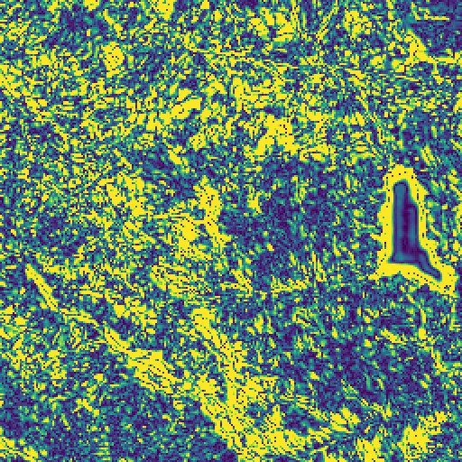
4.2. 20m and 60m resolution networks                                      Algorithm 1 DSen2. Network architecture.
   To avoid confusion between bands and simplify notation, we             Require: high-resolution bands (A): yA , low-resolution bands
collect bands that share the same GSD into three sets A =                   (B, C): yk , feature dimensions f , number of ResBlocks: d
{B2, B3, B4, B8} (GSD=10 m), B = {B5, B6, B7, B8a,                          # Cubic interpolation of low resolution:
B11, B12} (GSD=20 m) and C = {B1, B9} (GSD=60 m).                           Upsample yk to y   ek
The spatial dimensions of the high-resolution bands in A are                # Concatenation:
W × H. Further, let yA ∈ RW ×H×4 , yB ∈ RW/2×H/2×6 ,                        x0 := [yA , y
                                                                                        ek ]
and yC ∈ RW/6×H/6×2 denote, respectively, the observed in-                  # First Convolution and ReLU:
tensities of all bands contained in sets A, B and C respec-                 x1 := max(conv(x0 , f ), 0)
tively. As mentioned above, we train two separate networks for              # Repeat the ResBlock module d times:
different super-resolution factors. This reflects our belief that           for i = 1 to d do
self-similarity may progressively degrade with increasing scale                xi = ResBlock(xi−1 , f )
difference, such that 120→60 m is probably a worse proxy for                end for
20→10 m than the less distant 40→20 m.                                      # Last Convolution to match the output dimensions:
   The first network upsamples the bands in B using informa-                # (where klast is the last element in k)
tion from A and B:                                                          xd+1 := conv(xd , bklast )
                                                                            # Skip connection:
        T2× : RW ×H×4 × RW/2×H/2×6 → RW ×H×6                  (1a)          return x := xd+1 + y    eklast
               (yA , yB ) 7→ xB ,                             (1b)

where xB ∈ RW ×H×6 denotes the super-resolved 6-band im-                  yC to the target resolution (10 m) with simple bicubic interpo-
age with GSD 10 m. The second network upsamples C, unsing                 lation, to obtain y eB ∈ RW ×H×6 and y     eC ∈ RW ×H×2 . The
information from A, B and C:                                              inputs and outputs depend on whether the network T2× or S6×
                                                                          is used. To avoid confusion we define the set k of low resolu-
       S6× : RW ×H×4 × RW/2×H/2×6 × RW/6×H/6×2                            tion bands as is either k = {B} or k = {B, C}, respectively.
              → RW ×H×2                                       (2a)        The input is accordingly generalised as yk and the output as
                                                                          y
                                                                          eklast = yeB and y  eklast = y
                                                                                                       eC , where klast is the last element in
             (yA , yB , yC ) 7→ xC ,                          (2b)
                                                                          k. The proposed network architecture consists mainly of con-
with xC ∈ RW ×H×2 again the super-resolved 2-band image of                volutional layers, ReLU non-linearities and skip connections.
GSD 10 m.                                                                 A graphical overview of the network is given in Fig. 5, pseudo-
                                                                          code for the network specification is given in Algorithm 1.
4.3. Basic architecture                                                      The operator conv(x, fout ) represents a single convolution
                                                                          layer, i.e., a multi-dimensional convolution of image z with ker-
   Our network design was inspired by EDSR (Lim et al., 2017),            nel w, followed by an additive bias b:
the state-of-the-art in single-image super-resolution and winner
of the NTIRE super-resolution challenge (Timofte et al., 2017).                           v = conv(x, fout ) := w ∗ z + b                 (3)
EDSR follows the well-known ResNet architecture (He et al.,
2016) for image classification, which enables the use of very                    w : (fout × fin × k × k), b : (fout × 1 × 1 × 1)
deep networks by using the so called “skip connections”. These                         z : (fin × w × h), v : (fout × w × h)
long-range connections bypass portions of the network and are
added again later, such that skipped layers only need to esti-            where ∗ is the convolution operator. The convolved image v
mate the residual w.r.t. their input state. In this way the average       has the same spatial dimensions (w × h) as the input, the con-
effective path length through the network is reduced, which al-           volution kernels w and biases b, have dimensions (k × k). We
leviates the vanishing gradient problem and greatly accelerates           always use k = 3, in line with the recent literature, which sug-
the learning.                                                             gests that many layers of small kernels are preferable. The out-
   Our problem however, is different from classical single-               put feature dimension fout of the convolution depends only on
image super-resolution. In the case of Sentinel-2, the network            w and is required as an input. The input feature dimensions fin
does not need to hallucinate the high-resolution texture only on          depend only on the input image z and are adapted accordingly.
the basis of previously seen images. Rather, it has access to             The weights w and b are the free parameters learned during
the high-resolution bands to guide the super-resolution, i.e., it         training and what has to be ultimately learned by the network.
must learn to transfer the high-frequency content to the low-                The rectified linear unit (ReLU ) is a simple non-linear func-
resolution input bands, and do so in such a way that the re-              tion that truncates all negative responses in the output to 0:
sulting (high-resolution) pixels have plausible spectra. Con-
trary to EDSR, where the upsampling takes place at the end,                                        v = max(z, 0).                         (4)
we prefer to work with the high (10 m) resolution from the be-
ginning, since some input bands already have that resolution.                A residual block v = ResBlock(z, f ) is defined as a series
We thus start by upsampling the low-resolution bands yB and               of layers that operate on an input image z to generate an output
                                                                      6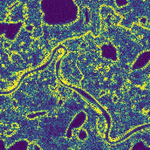
ResBlock

                       Upsample                            Upsample                                        Input

   Concatenation                       Concatenation                                                                      conv

        conv                                conv                                                                          ReLU
                                                                                                    skip connection
       ReLU                                ReLU                                                                           conv
     ResBlock                            ResBlock                                                                     Resid. Scaling

               times                               times

     ResBlock                            ResBlock
        conv                                conv                                                          Addition
                                                                                                           Output

                       Addition                            Addition                           Figure 6: Expanded view of the Residual Block.

Figure 5: The proposed networks T2× and S6× , with multiple ResBlock mod-        additive correction from the bicubically upsampled image to the
ules. The two networks differ only to the inputs.                                desired output. The strategy to predict the differences from a
                                                                                 simple, robust bicubic interpolation, rather than the final output
                                                                                 image, helps to preserve the radiometry of the input image.
z4 , then adds that output to the input image:
                                                                                 4.4. Deep and Very Deep networks
         z1 = conv(z, f )              #convolution                   (5a)
         z2 = max(z1 , 0)              #ReLU layer                    (5b)          Finding the right size and capacity for a CNN is largely an
                                                                                 empirical choice. Conveniently, the CNN framework makes it
         z3 = conv(z2 , f )            #convolution                   (5c)
                                                                                 possible to explore a range of depths with the same network de-
         z4 = λ · z3                   #residual scaling              (5d)       sign, thus providing an easy way of exploring the trade-off be-
          v = z4 + z                   #skip connection               (5e)       tween small, efficient models and larger, more powerful ones.
                                                                                 Also in our case, it is hard to know in advance how complex
   λ is a custom layer (5d) that multiplies its input activations                the network must be to adequately encode the super-resolution
(multi-dimensional images) with a constant. This is also termed                  mapping. We introduce two configurations of our ResNet ar-
residual scaling and greatly speeds up the training of very deep                 chitecture, a deep (DSen2) and a very deep one (VDSen2).
networks (Szegedy et al., 2017). In our experience residual                      The names are derived from Deep Sentinel-2 and Very Deep
scaling is crucial and we always use λ = 0.1. As a alter-                        Sentinel-2, respectively. For the deep version we use d = 6
native, we also tested the more common Batch Normalization                       and f = 128, corresponding to 14 convolutional layers, respec-
(BN), but found that it did not improve accuracy or training                     tively 1.8 million tunable weights. For the very deep one we set
time, while increasing the parameters of the network. Also, Lim                  d = 32 and f = 256, leading to 66 convolutional layers and a
et al. (2017) report that BN normalises the features and thus re-                total of 37.8 million tunable weights. DSen2 is comparatively
duces the range flexibility (the actual reflectance) of the images.              small for a modern CNN. The design goal here was a light net-
Within each ResBlock module we only include a ReLU after                         work that is fast in training and prediction, but still reaches good
the first convolution, but not after the second, since our net-                  accuracy. VDSen2 has a lot higher capacity, and was designed
work shall learn corrections to the bicubically upsampled im-                    with maximum accuracy in mind. It is closer in terms of size
age, which can be negative. Within our network design, the                       and training time to modern high-end CNNs for other image
ResBlock module can be repeated as often as desired. We show                     analysis tasks (Simonyan and Zisserman, 2015; He et al., 2016;
experiments with two different numbers d of ResBlocks: 6 and                     Huang et al., 2017), but is approximately two times slower and
32. The final convolution at the end of the network (after the                   five times slower in both training and prediction respectively,
multiple ResBlocks) reduces the feature dimensions to bklast ,                   compared to its shallower counterpart (DSen2). Naturally, one
such that they match the number of the required output bands                     can easily construct intermediate versions by changing the cor-
(xB and xC ). Concretely, if T2× is used bklast = 6 and if S6× is                responding parameters d and f . The optimal choice will depend
used bklast = 2.                                                                 on the application task as well as available computational re-
   A particularity of our network architecture is a long, additive               sources. On the one hand, the very deep variant is consistently
skip connection directly from the rescaled input to the output                   a bit better, while training and applying it is not more difficult,
(Fig. 5). This means that the complete network in fact learns the                if adequate resources (i.e., high-end GPUs) are available. How-
                                                                             7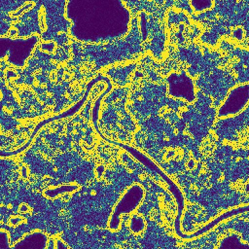
ever, the gains are small compared to the 20× increase in free
                                                                                              Table 2: Training and testing split.
parameters, and it is unlikely that going even deeper will bring
much further improvement.                                                              Images                       Split            Patches
                                                                                                    Training        90%       324’000 × 322
                                                                                         45
4.5. Training details                                                          T2×                 Validation       10%        36’000 × 322
   As loss function we use the mean absolute pixel error (L1                             15           Test                      15 × 5’4902
norm) between the true and the predicted high-resolution im-                                        Training        90%         20’250 × 962
age. Interestingly, we found the L1 norm to converge faster and                          45
                                                                               S6×                 Validation       10%          2’250 × 962
deliver better results than the L2 norm, even though the latter
                                                                                         15           Test                       15 × 1’8302
serves as error metric during evaluation. Most likely this is due
to the L1 norm’s greater robustness of absolute deviations to
outliers. We did observe that some Sentinel-2 images contain
                                                                           and has 9× more high-resolution pixels than for T2× ). Out of
a small number of pixels with very high reflectance, and due
                                                                           these patches 90% are used for training the weights, the remain-
to the high dynamic range these reach extreme values without
                                                                           ing 10% serve as validation set, see Table 2. To test the net-
saturating.
                                                                           works, we run both on the 15 full test images, each with a size
   Our learning procedure is standard: the network weights
                                                                           of 110×110 km2 , which corresponds to 5’490×5’490 pixels at
are initialised to small random values with the HeUniform
                                                                           20 m GSD, or 1’830×1’830 pixels at 60 m GSD.
method (He et al., 2015), and optimised with stochastic gra-
                                                                              Each network is implemented in the Keras framework (Chol-
dient descent (where each gradient step consists of a forward
                                                                           let et al., 2015), with TensorFlow as back-end. Training is run
pass to compute the current loss over a small random batch of
                                                                           on a NVIDIA Titan Xp GPU, with 12 GB of RAM, for approx-
image patches, followed by back-propagation of the error sig-
                                                                           imately 3 days. The mini-batch size for SGD is set to 128 to fit
nal through the network). In detail, we use the Adam variant of
                                                                           into GPU memory. The initial learning rate is lr = 1e-4 and it
SGD (Kingma and Ba, 2014) with Nesterov momentum (Dozat,
                                                                           is reduced by a factor of 2 whenever the validation loss does not
2015). Empirically, the proposed network architecture con-
                                                                           decrease for 5 consecutive epochs. For numerical stability we
verges faster than other ones we experimented with, due to the
                                                                           divide the raw 0 − 10’000 reflectance values by 2’000 before
ResNet-style skip connections.
                                                                           processing.
   Sentinel-2 images are too big to fit them into GPU memory
for training and testing, and in fact it is unlikely that long-range
context over distances of a kilometer or more plays any sig-               5.2. Baselines and Evaluation metrics
nificant role for super-resolution at the 10 m level. With this               As baselines, we use the methods of Lanaras et al. (2017) –
in mind, we train the network on small patches of w × h =                  termed SupReME, Wang et al. (2016) – termed ATPRK, and
(32 × 32) for T2× , respectively (96 × 96) pixels for S6× . We             Brodu (2017) – termed Superres. Moreover, as elementary
note that this corresponds to a receptive field of several hundred         baseline we use bicubic interpolation, to illustrate naive upsam-
metres on the ground, sufficient to capture the local low-level            pling without considering spectral correlations. Note, this also
texture and potentially also small semantic structures such as             directly shows the effect of our network, which is trained to re-
individual buildings or small waterbodies, but not large-scale             fine the bicubically upsampled image. The input image sizes
topographic features. We do not expect the latter to hold much             for the baselines were chosen to obtain the best possible re-
information about the local pixel values, instead there is a cer-          sults. SupReME showed the best performance when run with
tain danger that the large-scale layout of a limited training set it       patches of 256, respectively 240 for S6× and T2× . We specu-
is too unique to generalise to unseen locations.                           late that this may be due to the subspace projection used within
   As our network is fully convolutional, at the prediction step           SupReME, which can better adapt to the local image content
we can process image tiles of arbitrary size, limited only by the          with moderate tile size. The remaining baselines performed
on-board memory on the GPU. To avoid any potential boundary                best on full resolution images. The parameters for all baselines
artifacts from tiling, adjacent tiles are cropped with an overlap          were set as suggested in the original publications. This lead to
of 2 low-resolution input pixels, corresponding to 40 m for T2× ,          rather consistent results across the test set.
respectively 120 m for S6× .                                                  The main evaluation metric of our quantitative comparison is
                                                                           the root mean squared error (RMSE), estimated independently
                                                                           per spectral band:
5. Experimental Results
                                                                                                        r
                                                                                                           1X
5.1. Implementation details                                                                  RMSE =              (x̂ − x)2 ,              (6)
                                                                                                          n
   As mentioned before, we aim for global coverage. We there-
fore sample 60 representative scenes from around the globe, 45             where x̂ is each reconstructed band (vectorised), x is the vec-
for training and 15 for testing. For T2× we sample 8’000 ran-              torised ground truth band and n the number of pixels in x.
dom patches per training image, for a total of 360’000 patches.            The unit of the Sentinel-2 images is reflectance multiplied by
For S6× , we sample 500 patches per image for a total of 22’500            10’000, however, some pixels on specularities, clouds, snow
(note that each patch covers a 9× larger area in object space              etc. exceed 10’000. Therefore, we did not apply any kind of
                                                                       8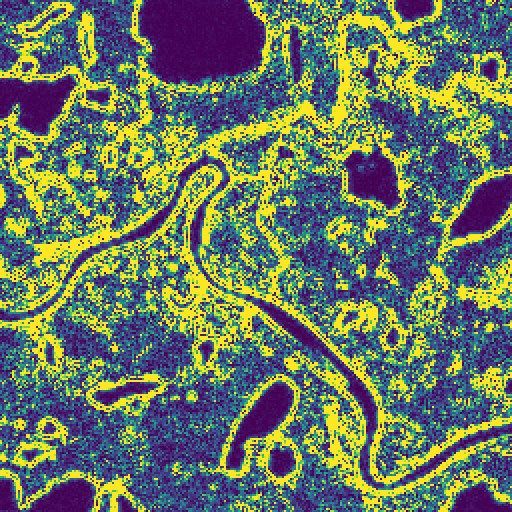
normalisation, and report RMSE values in the original files’
                                                                          Table 3: Aggregate results for 2× upsampling of the bands in set B, evaluated
value range, meaning that a residual of 1 corresponds to a re-            at lower scale (input 40 m, output 20 m).
flectance error of 10−4 .
                                                                                               Training RMSE           SRE       SAM        UIQ
   Depending on the scene content, some images have higher
reflectance values than others, and typically also higher abso-               Bicubic             123.5                 25.3      1.24     0.821
lute reflectance errors. To compensate for this effect, we also               ATPRK               116.2                 25.7      1.68     0.855
compute the signal to reconstruction error ratio (SRE) as ad-                 SupReME              69.7                 29.7      1.26     0.887
ditional error metric, which measures the error relative to the               Superres             66.2                 30.4      1.02     0.915
power of the signal. It is computed as:                                       DSen2 (ours) 40→20 34.5                   36.0      0.78     0.941
                                                                              VDSen2 (ours) 40→20 33.7                  36.3      0.76     0.941
                                       µ2x
                 SRE = 10 log10                ,               (7)            DSen2 (ours) 80→40              51.7      32.6      0.89     0.924
                                  kx̂ − xk2 /n                                VDSen2 (ours) 80→40             51.6      32.7      0.88     0.925
where µx is the average value of x. The values of SRE are given
in decibels (dB). We point out that using SRE, which measures
errors relative to the mean image intensity, is better suited to          the leap from the best baseline to DSen2 the differences may
make errors comparable between images of varying brightness.              seem small, but note that 0.3 dB would still be considered a
Whereas the popular peak signal to noise ratio (PSNR) would               marked improvement in many image enhancement tasks. In-
not achieve the same effect, since the peak intensity is constant.        terestingly, ATPRK and SupReME yield rather poor results for
Moreover, we also compute the spectral angle mapper (SAM),                SAM (relative spectral fidelity). Among the baselines, only Su-
i.e., the angular deviation between true and estimated spectral           perres beats bicubic upsampling. Our method again wins com-
signatures (Yuhas et al., 1992). We compute the SAM for each              fortably, more than doubling the margin between the strongest
pixel and then average over the whole image. The values of                competitor Superres and the simplistic baseline of bicubic up-
SAM are given in degrees. This metric is complimentary to the             sampling.
two previous ones, and quite useful for some applications, in                In the second test, we train an auxiliary T2× network on
that it measures how faithful the relative spectral distribution of       80→40 m instead of the 40→20 m, but nevertheless evaluate
a pixel is reconstructed, while ignoring absolute brightness. Fi-         it on the 20 m ground truth (while the model has never seen
nally, we report the universal image quality index (UIQ) (Wang            a 20 m GSD image). Of course this causes some drop in per-
and Bovik, 2002). This metric evaluates the reconstructed im-             formance, but the performance stays well above all baselines,
age in terms of luminance, contrast, and structure. UIQ is unit-          across all bands. I.e., the learned mapping is indeed suffi-
less and its maximum value is 1.                                          ciently scale-invariant to beat state-of-the-art model-based ap-
                                                                          proaches, which by construction should not depend on the abso-
5.3. Evaluation at lower scale                                            lute scale. For our actual setting, train on 40→20 m then use for
   Quantitative evaluation on Sentinel-2 images is only possi-            20→10 m, one would expect even a smaller performance drop
ble at the lower scale at which the models are trained. I.e., T2×         (compared to train on 80→40 m then use for 40→20 m), be-
is evaluated on the task to super-resolve 40→20 m, where the              cause of the well-documented inverse relation between spatial
40 m low-resolution and 20 m high-resolution bands are gen-               frequency and contrast in image signals (e.g., Ruderman, 1994;
erated by synthetically degrading the original data – for de-             van der Schaaf and van Hateren, 1996; Srivastava et al., 2003).
tails see Sec. 4.1. In the same way, S6× is evaluated on the              This experiment justifies our assumption, at 2× reduced reso-
super-resolution task from 360→60 m. Furthermore, to support              lution, that training 40→20 m super-resolution on synthetically
the claim that the upsampling function is to a sufficient degree          degraded images is a reasonable proxy for the actual 20→10 m
scale-invariant, we also run a test where we train T2× on the             upsampling of real Sentinel-2 images. We note that this re-
upsampling task from 80→40 m, and then test that network to               sult has potential implications beyond our specific CNN ap-
the 40→20 m upsampling task. In the following, we separately              proach. It validates the general procedure to train on lower-
discuss the T2× and S6× networks.                                         resolution imagery, that has been synthesised from the original
                                                                          sensor data. That procedure is in no way specific to our techni-
T2× — 20 m bands. We start with results for the T2× network,              cal implementation, and in all likelihood also not to the sensor
trained for super-resolution of actual S2 data to 10 m. Av-               characteristics of Sentinel-2.
erage results over all 15 test images and all bands in B =                   Tables 4 and Fig. 7 show detailed per-band results. The large
{B5,B6,B7,B8a,B11,B12} are displayed in Table 3. The state-               advantage for our method is consistent across all bands, and in
of-the-art methods SupReME and Superres perform similar,                  fact particularly pronounced for the challenging extrapolation
with Superres slightly better in all error metrics. DSen2 re-             to B11 and B12. We point out that the RMSE values for B6, B7
duces the RMSE by 48% compared to the previous state-of-                  and B8a are higher than for the other bands (with all methods).
the-art. The other error measures confirm this gulf in perfor-            In these bands also the reflectance is higher. The relative errors,
mance (>5 dB higher SRE, 24% lower SAM). VDSen2 further                   as measured by SRE, are very similar. Among our two net-
improves the results, consistently over all error measures (ex-           works, VDSen2 holds a moderate, but consistent benefit over
cept UIQ, where their scores are exactly the same). Relative to           its shallower counterpart across all bands, in both RMSE and
                                                                      9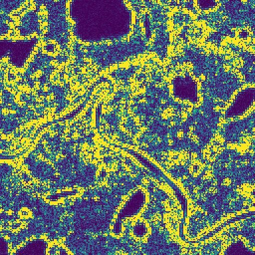
0.95
       150                                                  35
                                                                                                               0.90
       100
RMSE

                                                            30

                                                      SRE

                                                                                                         UIQ
                                                                                                               0.85
       50                                                   25
                                                                                                               0.80
             B5   B6     B7 B8a B11 B12                          B5    B6      B7 B8a B11 B12            B5                  B6     B7 B8a B11 B12
                           Bands                                                Bands                                                Bands
                         Bicubic   ATPRK                     SupReME              Superres   DSen2 (ours)                         VDSen2 (ours)

                                                      Figure 7: Per-band error metrics for 2× upsampling.

Table 4: Per-band values of RMSE, SRE and UIQ, for 2× upsampling. Values are averages over all test images. Evaluation at lower scale (input 40 m, output 20 m).
                                                              B5        B6           B7       B8a        B11          B12
                                                                                    RMSE
                                      Bicubic               105.0      138.1        159.3    168.3       92.4         78.0
                                      ATPRK                  89.4      119.1        136.5    147.4      113.3         91.7
                                      SupReME                48.1       70.2         78.6     82.9       76.5         61.7
                                      Superres               50.2       66.6         76.8     82.0       66.9         54.5
                                      DSen2                  27.7       37.6         42.8     43.8       29.0         26.2
                                      VDSen2                 27.1       37.0         42.2     43.0       28.0         25.1
                                                                                     SRE
                                      Bicubic                 25.1      25.6         25.4      25.5      26.3         24.0
                                      ATPRK                   26.6      26.9         26.7      26.6      24.7         22.7
                                      SupReME                 31.2      31.0         31.0      31.2      27.9         26.1
                                      Superres                31.3      31.7         31.4      31.4      29.1         27.2
                                      DSen2                   36.2      36.5         36.5      36.9      36.3         33.6
                                      VDSen2                  36.5      36.8         36.7      37.1      36.7         34.0
                                                                                     UIQ
                                      Bicubic               0.811      0.801        0.802    0.806      0.857     0.847
                                      ATPRK                 0.889      0.881        0.891    0.883      0.789     0.795
                                      SupReME               0.889      0.890        0.894    0.894      0.878     0.879
                                      Superres              0.918      0.920        0.921    0.919      0.904     0.905
                                      DSen2 (ours)          0.943      0.942        0.942    0.935      0.943     0.940
                                      VDSen2 (ours)         0.939      0.944        0.938    0.943      0.946     0.935

SRE. In terms of UIQ, they both rank well above the competi-                        for one of the test images. Yellow denotes high residual errors,
tion, but there is no clear winner. We attribute this to limitations                dark blue means zero error. For bands B6, B7, B8a and B11 all
of the UIQ metric, which is a product of three terms and thus                       baselines exhibit errors along high-contrast edges (the residual
not overly stable near its maximum of 1.                                            images resemble a high-pass filtering), meaning that they either
   It is interesting to note that the baselines exhibit a marked                    blur edges or exaggerate the contrast. Our method shows only
drop in accuracy for bands B11 and B12, whereas our networks                        traces of this common behaviour, and has visibly lower residu-
reconstruct B11 as well as other bands and show only a slight                       als in all spectral bands.
drop in relative accuracy for B12. These two bands lie in the
SWIR (>1.6µm) spectrum, far outside the spectral range cov-                         S6× — 60 m bands. For 6× super-resolution we train a sepa-
ered by the high-resolution bands (0.4–0.9µm). Especially AT-                       rate network, using synthetically downgraded images with 60 m
PRK performs poorly on B11 and B12. The issue is further                            GSD as ground truth. The baselines are run with the same set-
discussed in Sec. 5.5.                                                              tings as before (i.e., jointly super-resolving all input bands), but
   In Fig. 8, we compare reconstructed images to ground truth                       only the 60 m bands C = {B1, B9} are displayed. Overall and
                                                                               10
Bicubic ATPRK SupReME Superres DSen2 (ours) VDSen2 (ours)
B5
B6
B7
B8a
B11
B12
0 25 50 75 100 125 150 175 200
Figure 8: Absolute differences between ground truth and 2× upsampled result at 20 m GSD. The images show (absolute) reflectance differences on a reflectance
scale from 0 to 10, 000. Top, left to right: RGB (B2, B3, B4) image, color composites of bands (B5, B6, B7), and of bands (B8a, B11, B12). The image depicts the
Siberian tundra near the mouth of the Pur River.
11Table 5: Full results and detailed RMSE, SRE and UIQ values per spectral band. The results are averaged over all images for the 6× upsampling, with evaluation
at lower scale (input 360 m, output 60 m).
B1 B9 Average
SAM
RMSE SRE UIQ RMSE SRE UIQ RMSE SRE UIQ
Bicubic 171.8 22.3 0.404 148.7 17.1 0.368 160.2 19.7 0.386 1.79
ATPRK 162.9 22.8 0.745 127.4 18.0 0.711 145.1 20.4 0.728 1.62
SupReME 114.9 25.2 0.667 56.4 24.5 0.819 85.7 24.8 0.743 0.98
Superres 107.5 24.8 0.566 92.9 20.8 0.657 100.2 22.8 0.612 1.42
DSen2 33.6 35.6 0.912 30.9 29.9 0.886 32.2 32.8 0.899 0.41
VDSen2 27.6 37.9 0.921 24.4 32.3 0.899 26.0 35.1 0.910 0.34
Bicubic ATPRK SupReME Superres DSen2 (ours) VDSen2 (ours)
B1
B9
0 25 50 75 100 125 150 175 200
Figure 9: Absolute differences between ground truth and 6× upsampled result at 60 m GSD. The images show (absolute) reflectance differences on a reflectance
scale from 0 to 10, 000. Top: True scene RGB (B2, B3, B4), and false color composite of B1 and B9. This image depicts Berg River Dam in the rocky Hotentots
Holland, east of Cape Town, South Africa.
per-band results are given in Table 5. Once again, our DSen2 form better (relative to average radiance) on B1 than on B9.
network outperforms the previous state-of-the-art by a large The latter is the most challenging band for super-resolution,
margin, reducing the RMSE by a factor of ≈3. For the larger and the only one for which our SRE drops below 33 dB, and
upsampling factor, the very deep VDSen2 beats the shallower our UIQ below 0.9. It is worth noticing, that in this more
DSen2 by a solid margin, reaching about 20% lower RMSE, challenging 6× super-resolution, our method brings a bigger
respectively 2.3 dB higher SRE. improvement compared to the state-of-the-art baselines in 2×
Among the baselines, SupReME this time exhibits better super-resolution.
overall numbers than Superres, thanks to it clearly superior per-
formance on the B9 band. Contrary to the 2× super-resolution, We also present a qualitative comparison to ground truth,
all baselines improve SAM compared to simple bicubic in- again plotting absolute residuals in Fig. 9. As for 20 m, the
terpolation. Our method again is the runaway winner, with visual impression confirms that DSen2 and VDSen2 clearly
VDSen2 reaching 65% lower error than the nearest competitor dominate the competition, with much lower and less structured
SupReME. Looking at the individual bands, all methods per- residuals.
12Figure 10: Results of DSen2 on real Sentinel-2 data, for 2× upsampling. From left to right: True scene RGB in 10 m GSD (B2, B3, B4), Initial 20 m bands,
Super-resolved bands (B12, B8a and B5 as RGB) to 10 m GSD with DSen2. Top: An agricultural area close to Malmö in Sweden. Middle: A coastal area at the
Shark Bay, Australia. Bottom: Central Park at Manhattan, New York, USA. Best viewed on computer screen.
5.4. Evaluation at the original scale sampling we show both bands (B1,B9). In all cases the super-
To verify that our method can be applied to true scale resolved image is clearly sharper and brings out additional de-
Sentinel-2 data, we super-resolve the same test images as be- tails compared to the respective input bands. At least visually,
fore, but feed the original images, without synthetic downsam- the perceptual quality of the super-resolved images matches
pling, to our networks. As said before, we see no way to obtain that of the RGB bands, which have native 10 m resolution.
ground truth data for a quantitative comparison, and therefore
have to rely on visual inspection. We plot the upsampled results 5.5. Suitability of Pan-sharpening methods
next to the low-resolution inputs, in Fig. 10 for 2× upsampling As discussed earlier, there is a conceptual difference between
and in Fig. 11 for 6× upsampling. For each upsampling rate, multi-spectral super-resolution and classical pan-sharpening, in
the figures show 3 different test locations with varying land that the latter simply “copies” high-frequency information from
cover. Since visualisation is limited to 3 bands at a time, we an overlapping or nearby high-resolution band, but cannot ex-
pick bands (B5, B8a, B12) for 2× upsampling. For 6× up- ploit the overall reflectance distribution across the spectrum.
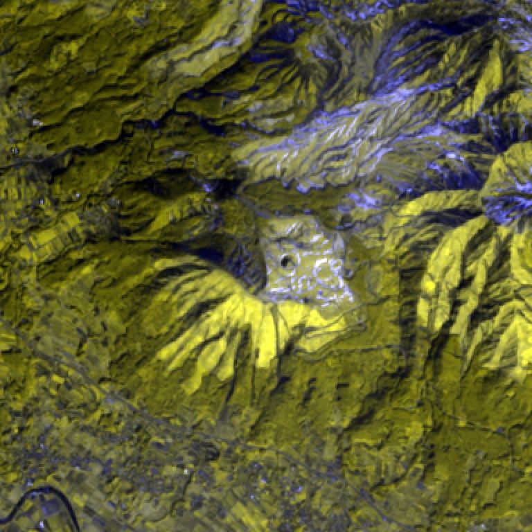
13Figure 11: Results of DSen2 on real Sentinel-2 data, for 6× upsampling. From left to right: True scene RGB (B2, B3, B4), Initial 60 m bands, Super-resolved
bands (B9, B9 and B1 as RGB) with DSen2. Top: London Heathrow airport and surroundings. Middle: The foot of Mt. Aso, on Kyushu island, Japan. Bottom: A
glacier in Greenland. Best viewed on computer screen.
14Table 6: Results of well-known pan-sharpening methods. RMSE, SRE and UIQ values per spectral band averaged over all images for the 2× upsampling, with
evaluation at lower scale (input 40 m, output 20 m).
B5 B6 B7 B8a B11 B12 Average
RMSE
Bicubic 105.0 138.1 159.3 168.3 92.4 78.0 123.5
PRACS 99.3 148.1 99.2 104.2 290.0 320.0 176.8
MTF-GLP-HPM-PP 91.0 66.5 77.6 82.7 78.7 240.6 106.2
BDSD 64.7 84.2 76.0 78.8 93.4 79.4 79.4
SRE
Bicubic 25.1 25.6 25.4 25.5 26.3 24.0 25.3
PRACS 24.0 24.2 28.7 29.0 19.5 14.4 23.3
MTF-GLP-HPM-PP 28.0 30.7 30.5 30.7 28.0 23.0 28.5
BDSD 28.3 29.2 31.1 31.5 26.3 23.9 28.4
UIQ
Bicubic 0.811 0.801 0.802 0.806 0.857 0.847 0.821
PRACS 0.836 0.858 0.882 0.881 0.791 0.773 0.837
MTF-GLP-HPM-PP 0.893 0.898 0.909 0.909 0.877 0.881 0.895
BDSD 0.866 0.892 0.909 0.908 0.858 0.848 0.880
Still, it is a-priori not clear how much of a practical impact reasonable SWIR bands for some images, but completely failed
this has, therefore we also test three of the best-performing on others, leading to excessive residuals. 4
pan-sharpening methods in the literature, namely PRACS (Choi While it may be possible to improve pan-sharpening perfor-
et al., 2011), MTF-GLP-HPM-PP (Lee and Lee, 2010) and mance with some sophisticated, perhaps non-linear combina-
BDSD (Garzelli et al., 2008). Quantitative error measures for tion for the pan-band, determining that combination is a re-
the 2× case are given in Table 6. Pan-sharpening requires a search problem on its own, and beyond the scope of this paper.
single “panchromatic” band as high-resolution input. The com- For readability, the pan-sharpening results are displayed in a
binations that empirically worked best for our data were the separate table. We note for completeness, that among the super-
following: For the near-infrared bands B6, B7 and B8a, we use resolution baselines (Tables 3 and 4), ATPRK is technically also
the broad high-resolution NIR band B8. As panchromatic band a super-resolution method. We categorise it as super-resolution,
for B5 we use B2, which surprisingly worked better than the since its creators also intend and apply it for that purpose. It can
spectrally closer B8, and also slightly better than other visual be seen in Table 4 that ATPRK actually also exhibits a distinct
bands. While for the SWIR bands there is no spectrally close performance drop for bands B11 and B12.
high-resolution band, and the best compromise appears to be Overall, we conclude that pan-sharpening cannot substitute
the average of the three visible bands, 31 (B2+B3+B4). qualified super-resolution, and is not suitable for Sentinel-2.
For bands B5, B6, B7 and B8 the results are reasonable: the Nevertheless, we point out that in the literature, the difficulties
errors are higher than those of the best super-resolution base- it has especially with bands B11 and B12 is sometimes masked,
line (and consequently 2-3× higher than with our networks, c.f . because many papers do not show the individual per-band er-
Table 4), but lower than naive bicubic upsampling. This con- rors.
firms that there is a benefit from using all bands together, rather
than the high-frequency data from only one, arbitrarily defined
6. Discussion
“panchromatic” band.
On the contrary, for the SWIR bands B11 and B12 the per- 6.1. Different network configurations
formance of pan-sharpening drops significantly, to a point that
The behaviour of our two tested network configurations is
the RMSE drops below that of bicubic interpolation (and simi-
in line with the recent literature: networks of moderate size
lar for SRE). As was to be expected, successful pan-sharpening
(by today’s standards), like DSen2, already perform fairly well.
is not possible with a spectrally distant band that has very dif-
Across a wide range of image analysis tasks from denoising to
ferent image statistics and local appearance. Moreover, pan-
instance-level semantic segmentation and beyond, CNNs with
sharpening is very sensitive to the choice of the “panchromatic”
around 10-20 layers have redefined the state-of-the-art. Over
band. We empirically picked the one that worked best on aver-
the last few years, improvements to the network architecture
age, but found that, for all tested methods, there isn’t one that
performs consistently across all test images. This is particularly
evident for MTF-GLP-HPM-PP. Even with the best pan-band 4 Actually, for MTF-GLP-HPM-PP we had to exclude one of the 15 images
we found (the average of the visible bands), it reconstructed from the evaluation, since the method did not produce a valid output.
15You can also read