Technical note: A view from space on global flux towers by MODIS and Landsat: the FluxnetEO data set
←
→
Page content transcription
If your browser does not render page correctly, please read the page content below
Technical note
Biogeosciences, 19, 2805–2840, 2022
https://doi.org/10.5194/bg-19-2805-2022
© Author(s) 2022. This work is distributed under
the Creative Commons Attribution 4.0 License.

Technical note: A view from space on global flux towers by MODIS
and Landsat: the FluxnetEO data set
Sophia Walther1, , Simon Besnard1,2, , Jacob Allen Nelson1 , Tarek Sebastian El-Madany1 , Mirco Migliavacca1,3 ,
Ulrich Weber1 , Nuno Carvalhais1,4 , Sofia Lorena Ermida5,6 , Christian Brümmer7 , Frederik Schrader7 ,
Anatoly Stanislavovich Prokushkin8 , Alexey Vasilevich Panov8 , and Martin Jung1
1 Department   Biogeochemical Integration, Max-Planck-Institute for Biogeochemistry, Hans-Knöll-Straße 10, Jena, Germany
2 South  Pole, Digital Innovation, Fred. Roeskestraat 115, Amsterdam, the Netherlands
3 European Commission, Joint Research Centre, Via Fermi 2749, Ispra (VA), Italy
4 Departamento de Ciências e Engenharia do Ambiente, DCEA, Faculdade de Ciências e Tecnologia, FCT,

Universidade Nova de Lisboa, 2829-516 Caparica, Portugal
5 Departamento de Ciências e Engenharia do Ambiente (DCEA), Faculdade de Ciências e Tecnologia (FCT), Universidade

Nova de Lisboa, Lisbon, Portugal
6 Instituto Dom Luiz, Faculdade de Ciências da Universidade de Lisboa, Campo Grande Edifício C1,

Piso 1, 1749-016 Lisbon, Portugal
7 Thünen Institute of Climate-Smart Agriculture, Bundesallee 65, Braunschweig, Germany
8 V.N. Sukachev Institute of Forest of the Siberian Branch of Russian Academy of Sciences – separated department of the

KSC SB RAS, Akademgorodok 50/28, Krasnoyarsk, Russia
 These authors contributed equally to this work.

Correspondence: Sophia Walther (sophia.walther@bgc-jena.mpg.de)

Received: 21 November 2021 – Discussion started: 25 November 2021
Revised: 4 April 2022 – Accepted: 5 April 2022 – Published: 8 June 2022

Abstract. The eddy-covariance technique measures carbon,          lites. The methods consistently process surface reflectance
water, and energy fluxes between the land surface and             in individual spectral bands, derived vegetation indices, and
the atmosphere at hundreds of sites globally. Collections         land surface temperature. A geometrical correction estimates
of standardised and homogenised flux estimates such as            the magnitude of land surface temperature as if seen from
the LaThuile, Fluxnet2015, National Ecological Observa-           nadir or 40◦ off-nadir. Finally, we offer the community living
tory Network (NEON), Integrated Carbon Observation Sys-           data sets of pre-processed Earth observation data, where ver-
tem (ICOS), AsiaFlux, AmeriFlux, and Terrestrial Ecosys-          sion 1.0 features the MCD43A4/A2 and MxD11A1 MODIS
tem Research Network (TERN)/OzFlux data sets are invalu-          products and Landsat Collection 1 Tier 1 and Tier 2 products
able to study land surface processes and vegetation function-     in a radius of 2 km around 338 flux sites. The data sets we
ing at the ecosystem scale. Space-borne measurements give         provide can widely facilitate the integration of activities in
complementary information on the state of the land surface        the eddy-covariance, remote sensing, and modelling fields.
in the surroundings of the towers. They aid the interpreta-
tion of the fluxes and support the benchmarking of terrestrial
biosphere models. However, insufficient quality and frequent
and/or long gaps are recurrent problems in applying the re-       1   Introduction
motely sensed data and may considerably affect the scien-
tific conclusions. Here, we describe a standardised proce-        The installation and maintenance of instrumental infrastruc-
dure to extract, quality filter, and gap-fill Earth observation   ture at eddy-covariance (EC) sites worldwide require consid-
data from the MODIS instruments and the Landsat satel-            erable financial and logistical efforts and labour force. The
                                                                  precious data sets of land–atmosphere fluxes, biometeorolog-

Published by Copernicus Publications on behalf of the European Geosciences Union.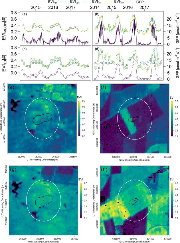
2806                                    S. Walther et al.: A view from space on global flux towers by MODIS and Landsat

ical data, and environmental conditions allow fundamental          cedure shall be as simple as possible, computationally effi-
insights into ecosystem functioning (Baldocchi, 2008; Bal-         cient, and not resort to additional data sources to facilitate a
docchi et al., 2018; Baldocchi, 2020; Besnard et al., 2018;        potential application to EO data at the global scale.
Migliavacca et al., 2021; Nelson et al., 2020). A signifi-            We apply the proposed processing steps to official data
cant achievement is the central processing, quality control,       products from the Moderate Resolution Imaging Spectrora-
and open standardised distribution of a large number of the        diometer (MODIS) instruments and the sensors on board the
available observational records in data collections such as        Landsat satellites. Both MODIS and Landsat have extensive
LaThuile, Fluxnet2015, and ABCflux (amongst others, Pa-            observational coverage with a high temporal overlap with
pale et al., 2006; Baldocchi, 2008; Pastorello et al., 2020;       most freely available EC records. Landsat measurements are
Virkkala et al., 2022; Papale, 2020) to which many site teams      of particular interest because they resolve small spatial de-
contribute.                                                        tails in pixels of 30 m size, but at the cost of missing out
   Complementary information from satellites or digital cam-       on short temporal features. The opposite is true for MODIS
eras (phenocams, Wingate et al., 2015) aids and refines            data products, which partly average over heterogeneous areas
studies of local land–atmosphere interactions as they relate       in spatially comparatively coarse pixels of several hundred
to ecosystem structure, phenology, and functioning and the         metres. However, MODIS offers daily, partly even sub-daily,
state of the land surface (e.g. Migliavacca et al., 2015; Bao      temporal resolution. We process EO data sets of surface re-
et al., 2022). Earth observation (EO) data for varying regional    flectance, vegetation indices, and land surface temperature
sizes around the sites can represent the actual area that con-     (LST) for a limited area around a given flux site.
tributes to the flux measurements – partly even more accu-            As missing data points in EO data are a ubiquitous prob-
rately than similar ground-based measurements can (Gamon,          lem, a number of related initiatives also provide access to
2015) – provided sufficiently high spatial resolution and tem-     EO data that underwent certain pre-processing. For example,
poral overlap with the site-level records. Next to local stud-     Robinson et al. (2017) offer 30 m Landsat NDVI for all pix-
ies, the combination of flux and satellite observations is also    els in the CONUS every 16 d between 1984–2019. They re-
a basic ingredient for upscaling exercises of the in situ fluxes   moved cloud effects and filled gaps with climatological aver-
to larger areas or even the globe (Ueyama et al., 2013; Tra-       ages. Moreno-Martínez et al. (2020) controlled Landsat and
montana et al., 2016; Jung et al., 2019, 2020; Joiner et al.,      MODIS surface reflectance for cloud, snow, and water effects
2018; Reitz et al., 2021; Virkkala et al., 2021; Zeng et al.,      and fused them to a gap-free and smoothed product. It covers
2020).                                                             surface reflectance and its uncertainty in six Landsat spectral
   Independent of the nature of the scientific application, the    bands at monthly, 30 m resolution for the CONUS and the
quality control and gap structure of both the EC and the EO        years 2009–2020. An example product for gap-free MODIS
data are the groundwork of each analysis. Different criteria       surface reflectance (as well as albedo and BRDF parameters)
help to identify problematic data points with differing levels     at approximately 1 km resolution is the MCD43GF product
of strictness depending on the given application. Moffat et al.    (Sun et al., 2017). In this case, the time series of the param-
(2007) and Falge et al. (2001) describe techniques to fill gaps    eters of the bidirectional reflectance distribution function are
due to missing data points in the EC data. The literature also     temporally and spatially gap-filled for days and pixels with
offers a diverse set of methods to gap-fill EO data that in-       bad inversion quality or cloud and snow influence, and from
clude spatial, temporal, cross-sensor, and cross-variable ap-      those gap-free model parameters a global gap-free product
proaches (to name a few, Wang et al., 2012; van Buttlar et al.,    of surface reflectance is provided for the MODIS land bands
2014; Weiss et al., 2014; Verger et al., 2011, 2013; Kan-          and three broad spectral bands. Finally, a sub-setting tool
dasamy et al., 2013; Moreno et al., 2014; Moreno-Martínez          (ORNL DAAC, 2018) facilitates access to a range of global
et al., 2020; Yan and Roy, 2018; Ghafarian Malamiri et al.,        EO data sets at a large selection of eddy-covariance sites.
2018; Li et al., 2018; Dumitrescu et al., 2020; Bessenbacher          FluxnetEO is unique in proposing the completion of all
et al., 2021). The pre-processing steps are laborious, and they    pre-processing steps necessary for scientific analysis at site
are key to the results and interpretation of the analyses.         level, hence resulting in an analysis-ready data set. The prod-
   We propose a set of systematic pre-processing steps for         ucts in version 1.0 of the data cover the period 1984–2017
key land surface indicators from EO data: sub-setting global       and 2000–2020 for Landsat and MODIS, respectively, and
EO data for an area around an EC site; systematic control          are freely available by the services of the ICOS Carbon Por-
for good-quality retrievals as well as cloud, snow, and wa-        tal (see data availability statement; Walther et al., 2021a, b).
ter effects; and estimating missing data points in a flexible      Each data set has a complementary data layer with additional
and ecologically meaningful way. For both the quality con-         flags to inform the user whether data points correspond to
trol and the gap filling, the approaches aim to be generalis-      actual good-quality observations according to the proposed
able across all sites without accounting for specific local con-   criteria and, if not, how they have been estimated in differ-
ditions, yet flexible enough to accurately reproduce pheno-        ent gap-filling steps. FluxnetEO provides a ready-to-use data
logical behaviour and characteristic features such as distur-      set, which, however, means limited flexibility for the users
bances or fast transitions in managed ecosystems. The pro-         to make their own decisions on the pre-processing steps.

Biogeosciences, 19, 2805–2840, 2022                                                   https://doi.org/10.5194/bg-19-2805-2022
S. Walther et al.: A view from space on global flux towers by MODIS and Landsat                                             2807

For example, they depend on the site selection made by the         shrublands and only one site from a deciduous needleleaf for-
authors (see Table E1 for the site selection in version 1.0)       est (Table 1).
and their decision to cover an area within a radius of 2 km
around a site. Conversely, the ORNL DAAC (2018) offers             2.2   MODIS and Landsat
larger cutout radii of 4 km around a considerably larger col-
lection of sites than FluxnetEO and from a complementary           The MCD43A4 product combines Aqua and Terra obser-
selection of global EO products. But users will need to invest     vations and provides estimates of surface reflectance in the
considerable work in quality control and gap filling. Regard-      MODIS bands 1–7 (Schaaf and Wang, 2015b). Time series
ing available quality-controlled and gap-free large-scale or       represent observations modelled at nadir view at a resolution
even global gridded EO data (Moreno-Martínez et al., 2020;         of 16 d and 500 m spatial pixels. For the quality control of
Robinson et al., 2017; Sun et al., 2017), the user needs to find   MCD43A4, a complementary product, MCD43A2, contains
ways to access these data sets at site level (while Moreno-        band-specific information on the quality of the inversion of
Martínez et al., 2020, is available on Google Earth Engine         the bidirectional reflectance distribution function as well as
(GEE), Sun et al., 2017, is not, and Robinson et al., 2017,        snow cover, platform information, and land–water coverage
needs shape files) and needs to understand whether the ap-         in the scene (Schaaf and Wang, 2015a).
plied quality filters match the needs of their application.           The MODIS MOD11A1 (Terra, starting in 2000) and
   To allow potential users to make an informed decision on        MYD11A1 (Aqua, starting in 2002) products (hereafter
the product which suits their application best, we describe de-    jointly referred to as MxD11A1, Wan et al., 2015a, b) pro-
tails about data inputs in FluxnetEO in Sect. 2.2, explain the     vide daily LST and emissivity estimates aligned with quality
quality control and gap-filling approaches in Sect. 3, illus-      and view angle information at 1 km spatial pixel sizes. The
trate examples, and benchmark the products against a selec-        LST values represent instantaneous values and are selected
tion of independent products and approaches in Sect. 4. Ta-        based on viewing zenith angle and LST values (MOD11A1
ble 2 and the data availability section provide detailed infor-    user guide, https://lpdaac.usgs.gov/documents/118/MOD11_
mation on the resulting products, while Table A1 summarises        User_Guide_V6.pdf, last access: 3 May 2022). Four LST
and compares the main characteristics of the selected studies      data streams are available: TERRAday with observations
and services mentioned above (Robinson et al., 2017; Sun           around 10:30 local time, AQUAday with observations around
et al., 2017; Moreno-Martínez et al., 2020; ORNL DAAC,             13:30 local time, TERRAnight around 22:30 local time and
2018) and the one in this contribution. We expect FluxnetEO        AQUAnight around 01:30 local time. For each of them, obser-
to be a living data set with regular updates regarding the site    vation times vary between overpasses by about ± 1.5 h.
selection, the temporal coverage, the release of new Land-            Observation geometries need special attention as the
sat/MODIS collections and processing improvements based            MODIS instruments measure in a wide swath to obtain high
on user feedback. Potential users are therefore advised to re-     temporal coverage. They scan across their track from right
fer to the ICOS Carbon Portal for the latest product version       to left with view zenith angles up to 65◦ from nadir. The
and site availability information (Walther et al., 2021a, b).      wide range of viewing geometries leads to different frac-
                                                                   tions of surface types seen from one overpass to the next for
                                                                   a given site. In addition, vegetation structure and topogra-
2     Data                                                         phy, together with the position of the sun relative to the sen-
                                                                   sors, cause variable shadowing effects. The reflectance prod-
2.1    Eddy-covariance sites                                       uct (MODIS MCD43A4, Schaaf and Wang, 2015b) partly
                                                                   accounts for these anisotropy effects and simulates a nadir
For the current version 1.0 of the product we select the           view. In order to partly account for variability in the ob-
338 sites from the LaThuile, Fluxnet2015 (Pastorello et al.,       served LST that is related to changing observation geome-
2020), and ICOS Drought 2018 Initiative (Drought 2018              try (Rasmussen et al., 2011; Guillevic et al., 2013; Ermida
Team and ICOS Ecosystem Thematic Centre, 2020) flux data           et al., 2014), a correction approach developed by Ermida
releases. Site coordinates given in different sources (Ameri-      et al. (2018) estimates an LST offset as if the instrument were
Flux, AsiaFlux, Europe-Fluxdata, Fluxdata.org, and a previ-        measuring from directly above a site. For some applications,
ously compiled in-house Fluxnet site location list) may dif-       an oblique view might be favourable over a nadir constella-
fer. In that case, the coordinates with the highest precision      tion, for example to enhance the contribution of vegetation
were selected. In case the coordinates differed by more than       canopy to the LST estimate and minimise fractions of soil
0.001◦ for a given site, a manual check in Google Earth iden-      or understorey. In addition, we provide LST corrected to a
tified the correct or most probable location of the site. The      viewing zenith angle of 40◦ .
final set of 338 sites for which we process the MODIS and             Reflectance-based Landsat time series comprise the en-
Landsat EO data in product version 1.0 is listed in Table E1.      tire multi-temporal collection 1 of the Landsat 4, 5, 7,
Forests and grasslands are best represented among the 338          and 8 archives (https://landsat.gsfc.nasa.gov/data, last ac-
sites. The collection includes fewer sites from savannas and       cess: 3 May 2022) covering the period 1984–2017 at

https://doi.org/10.5194/bg-19-2805-2022                                                   Biogeosciences, 19, 2805–2840, 2022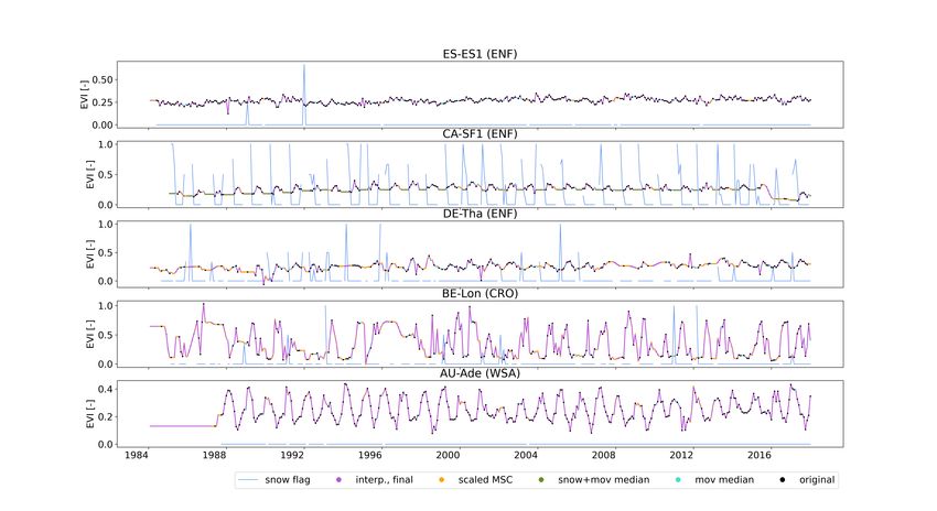
2808                                        S. Walther et al.: A view from space on global flux towers by MODIS and Landsat

Table 1. Representation of different plant functional types and Köppen climate classes across the 338 sites in the FluxnetEO v1.0 collection.

                    Plant functional type                  Number of sites       Köppen main climate    Number of sites
                    Evergreen needleleaf forest (ENF)                    86      Arid                                26
                    Evergreen broadleaf forest (EBF)                     25      Equatorial                          23
                    Deciduous needleleaf forest (DNF)                     1      Warm temperate                     171
                    Deciduous broadleaf forest (DBF)                     40      Snow                               103
                    Mixed forest (MF)                                    13      Polar                               12
                    Woody savanna (WSA)                                  10      Undefined                            3
                    Savanna (SAV)                                        11
                    Closed shrubland (CSH)                                6
                    Open shrubland (OSH)                                 19
                    Grassland (GRA)                                      58
                    Crops (CRO)                                          36
                    Wetlands (WET)                                       32
                    Snow (SNO)                                            1

30 m spatial pixel size. The seven spectral bands of the                 3     Methods
Landsat product were collected: blue, green, red, near
infrared (NIR), shortwave infrared 1 and 2 (SWIR1,                       We describe here the overall concept and rationale of the
SWIR2), and thermal infrared (TIR) (https://landsat.usgs.                quality filter and the gap filling, but we report all technical
gov/what-are-band-designations-landsat-satellites, last ac-              details in Appendix A.
cess: 3 May 2022). Landsat data have been pre-processed
using the Landsat Ecosystem Disturbance Adaptive Pro-                    3.1     Processing steps of reflectance-based indicators
cessing System (LEDAPS, Schmidt et al., 2013) and the
Landsat Surface Reflectance Code (LaSRC, https://landsat.                The processing steps for reflectance-based land surface vari-
usgs.gov/landsat-surface-reflectance-data-products, last ac-             ables can be summarised by the following steps:
cess: 3 May 2022) for atmospheric correction. The pixelQA                    1. quality control for effects of snow, water, bad inver-
layer contains information related to clouds, cloud shadows,                    sion per spectral band, and individual pixel in a cutout
snow, and water and is useful for the quality control of the                    (henceforth subpixel) using the MODIS/Landsat quality
Landsat data (Zhu and Woodcock, 2012; Zhu et al., 2015).                        flags;
In contrast to MODIS, the Landsat sensors acquire images
at much smaller view angles around 7.5◦ from nadir. Ground                   2. optionally compute vegetation index per subpixel, or
control points and a digital elevation model help to correct for                use the raw spectral bands;
small directional effects related to terrain structure and view-
ing angles (Wulder et al., 2019). Corrections for the small but              3. optionally spatially aggregate over a selection of sub-
significant differences between the spectral characteristics of                 pixels in the cutout to obtain one time series per site, or
Landsat ETM+ and OLI (Roy et al., 2016) are not applied.                        decide to process all subpixels individually;
    The services by GEE provided cutouts of the above-
mentioned products at the EC sites. Independently of the                     4. remove values of an index outside its defined ranges and
product and its spatial resolution, the cutout area was limited                 apply an additional outlier filter;
to a maximum distance of 2 km between a given tower and
the centre of a given satellite pixel. No single cutout size will            5. gap filling.
fit the flux footprint extents of all sites (Chu et al., 2021). The
                                                                         3.1.1     Quality control and computation of spectral
decision for a radius of 2 km in product version 1.0 compro-
                                                                                   indices
mises reasonable data set sizes and the inclusion of the high-
temporal-resolution flux footprints for the majority of sites.           Quality control of the MODIS reflectance-based vegetation
Downloading the EO data in tiff format avoided nontranspar-              indices focused on three aspects: good inversion quality
ent re-projection of the data from sinusoidal to regular grid            of the bidirectional reflectance distribution function as in-
by GEE, which would have been problematic for the quality                dicated by the BRDF_Albedo_Band_Quality_Bandx flags
flags in the MCD43A2 and MxD11A1 products. The Landsat                   in the MCD43A2 product, snow-free conditions according
data were already provided in regular grid by GEE.                       to the Snow_BRDF_Albedo flag, and the omission of re-
                                                                         flectance values that are affected by the presence of water in
                                                                         the field of view using the BRDF_Albedo_LandWaterType

Biogeosciences, 19, 2805–2840, 2022                                                            https://doi.org/10.5194/bg-19-2805-2022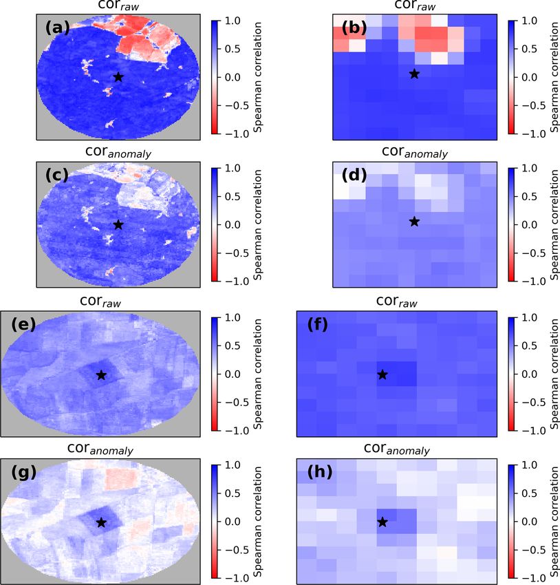
S. Walther et al.: A view from space on global flux towers by MODIS and Landsat                                             2809

flag. For the selected data samples which passed those cri-             but see details in Appendix A). Consider all times with
teria, we computed a large set of spectral vegetation indices           a snow flag larger than 0.1 or missing snow information
(Table 2). An additional check removed possible values of               as snow covered. The latter periods are included as the
the vegetation indices outside their defined ranges. Some               snow flag appears to systematically miss snow periods
of the time series contained obvious outlier values. We em-             in higher latitudes in the beginning of the winter. Still,
ployed an empirical filter which largely removed those sam-             frequent gaps with missing snow information also oc-
ples which had a particularly large difference to the median            cur during the growing season. In order to avoid wrong
of their surrounding values in a temporal window (Papale                filling with a constant value during the growing season,
et al., 2006, technical details on all filters in Appendix A).          this gap-fill step is not applied when the probability of
   In the Landsat data, the flag pixel_qa provided quality at-          snow cover is low, i.e. when the average seasonal cycle
tributes (CFMask, Foga et al., 2017) and removed pixels that            indicates typically snow-free conditions at a given time
contained snow/ice, water, cloud, and/or cloud shadow using             of the year, or when typically no snow occurs at all at a
a binary flag of presence. Similar to the MODIS product, we             given site.
computed a series of spectral vegetation indices (Table 2) us-
ing the good-quality observations and removed possible val-         3. Subsequently, another moving median in windows of
ues of the indices outside their defined ranges. A slightly            40 d (4 months for Landsat) fills gaps shorter than 65 d
modified filter removed possible outlier values also for the           (2 months for Landsat).
Landsat data (see details in Appendix A.).
                                                                    4. Linearly regress the time series on its own median sea-
3.1.2   Gap filling                                                    sonal cycle (MSC). Compute a re-scaled MSC with the
                                                                       obtained regression parameters and use it to fill longer
In the literature several gap-filling and smoothing approaches         gaps. Execute the regression and re-scaling in tempo-
are available which work in one or more dimensions (e.g.               ral moving windows as this guarantees more flexibil-
Wang et al., 2012; Kandasamy et al., 2013; van Buttlar et al.,         ity to correctly represent inter-annual variations in the
2014; Weiss et al., 2014; Yan and Roy, 2018; Zhang et al.,             time series and even partly accounts for changes in the
2021) or use fusion methods between sensors (Verger et al.,            shape of the seasonal cycle due to disturbances. It is,
2011; Moreno-Martínez et al., 2020). They differ in their lev-         however, not suited to fill regularly recurring gaps at a
els of sophistication and computational efforts. One of our            certain time of the year, e.g. during rain seasons (Verger
requirements for the gap-filling approach was that it employs          et al., 2013).
exclusively temporal operations and does not use additional
data sources. It is hence very generalisable and allows the gap     5. Fill the remaining gaps by piecewise cubic polynomial
filling to be generally applicable to a single time series per         interpolation. Time series with fewer than 300 valid data
site, several subpixels in a cutout around a site, and global EO       (12 months for Landsat) points in the whole record after
data. A number of possible applications will require the anal-         application of all the previous gap-filling steps will not
ysis of actual observations, and consequently approaches that          be meaningful for analysis but are still filled by nearest-
fit smooth functions to available good-quality data (e.g. Jon-         neighbour interpolation.
sson and Eklundh, 2002; Gonsamo et al., 2013) to represent
a gap-free time series are not suitable. Therefore, the idea        6. Temporal operations cannot meaningfully fill gaps at
was to retain the good-quality data and make as realistic of           the beginning and at the end of the record. Therefore
estimates as possible for the gaps between them. The follow-           the first (last) valid data points are repeatedly appended
ing recipe describes the steps to estimate missing data points         at the beginning (end) of the record.
conceptually; all technical details we report in Appendix A.          The described processing steps are generalisable across
Unless stated otherwise, for each gap-filling step, the values     a range of spectral vegetation indices and can reliably fill
filled in previous steps guide the current and subsequent gap-     missing data points across sites globally (see examples in
filling steps together with the good-quality observations.         Sect. 4). However, a number of sites have extremely low
 1. Fill short non-snow-related gaps (≤ 5 d or ≤ 1 month           data availability after quality checks, and the gaps in their
    for MODIS and Landsat, respectively) with a median             time series are challenging to temporally interpolate in a
    across valid values in moving windows of 16 d (3               meaningful way. This can lead to problematic gap-filled data
    months for Landsat). The moving median only fills              points with questionable reliability and realism. Examples
    gaps; it does not change/smooth valid data points.             are tropical sites and/or sites with a pronounced wet sea-
                                                                   son with permanent cloud cover. The same generally ap-
 2. Fill snow-related gaps with a constant baseline value          plies for MODIS in the years 2000–2002 when observa-
    which is identified as the average of valid data points        tions stem mainly from the Terra satellite, and therefore
    adjacent to snow-covered periods, i.e. immediately be-         data availability is comparatively low. For Landsat, the num-
    fore snowfall or after snowmelt (after Beck et al., 2007,      ber of available scenes is relatively heterogeneous across

https://doi.org/10.5194/bg-19-2805-2022                                                   Biogeosciences, 19, 2805–2840, 2022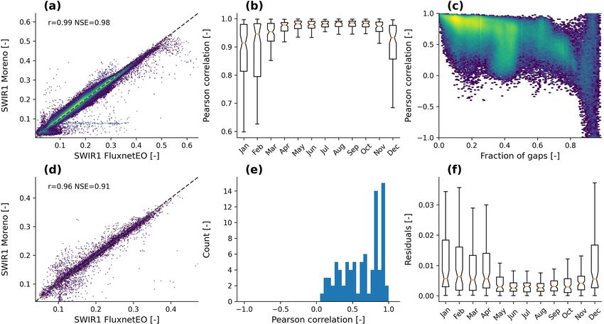
2810                                     S. Walther et al.: A view from space on global flux towers by MODIS and Landsat

the globe (https://www.usgs.gov/media/images/cumulative-            0.05◦ . We followed the pragmatic approach of selecting the
number-scenes-landsat-archive, last access: 3 May 2022),            model coefficients for the correction from the pixel contain-
with some regions having very good coverage (e.g. North             ing a given site. We acknowledge that we did not investigate
America) while other regions are observed less frequently           to what extent the given site conditions represent the overall
(e.g. Russia and Africa). Such differences in the availability      characteristics of the land surface in the allocated pixel. Fur-
of good-quality data between sites strongly affect the qual-        ther input to the geometrical model were the viewing azimuth
ity of the gap filling at the site level. In addition, FluxnetEO    angles, solar angles at the overpass time, and estimates of
provides for each data layer a gap-fill flag, consisting of a       daily potential radiation at the top of the atmosphere. The ge-
range of integer values to identify original good-quality data      ometrical correction was applied to each subpixel in a cutout
(flag = 0) from gap-filled estimates (flags = 1. . .n) where in-    separately.
formation is provided in which gap-filling step a certain data
sample has been imputed. This allows users to explore indi-         3.2.3   Gap filling
vidual sites and use (parts of) the gap-filled data or resort to
only using the high-quality original data points.                   Also for the gap filling of LST, several approaches are
                                                                    present in the literature (e.g. Gerber et al., 2018; Ghafar-
3.2     Preprocessing of MODIS land surface temperature             ian Malamiri et al., 2018; Li et al., 2018; Dumitrescu et al.,
                                                                    2020). When using exclusively operations in time and no an-
The processing of the LST follows this order:                       cillary data to estimate invalid LST observations, one needs
                                                                    to consider the shorter autocorrelation of LST compared to
  1. outlier filter for each LST data stream and check that
                                                                    the reflectance-based indicators. According to Vinnikov et al.
     any daytime LST is higher than any nighttime LST per
                                                                    (2008), the weather-related component of clear-sky LST has
     subpixel and day
                                                                    an autocorrelation of about 3 d. The following sequence of
  2. optionally apply a geometrical correction per subpixel         steps filled the four MODIS LST data streams (for technical
                                                                    details refer to Appendix B).
  3. optionally aggregate over a selection of subpixels in the
     cutout per time step and LST data stream                        1. Similar to the reflectances, a first step consisted of a
                                                                        temporal moving median in windows of 8 d to fill gaps.
  4. gap-fill the aggregated time series or each subpixel for
     all four MODIS LSTs simultaneously.                             2. A second step was inspired by Li et al. (2018) and
                                                                        Crosson et al. (2012) and foresaw using one of the four
3.2.1    Quality checks
                                                                        MODIS LST time series as a “reference” to fill gaps in
The quality control of the MODIS LST focused on removing                a second “imputed” one. We computed a MSC of the
outlier values. Negative outlier values in LST might represent          difference between the “reference” and the “imputed”
residual cloud contamination, whereas unusually high val-               MODIS LST. This average shift was linearly scaled to
ues might originate from undetected saturation in the level 1           the actual shift in temporal windows. The scaled aver-
data. We found that the flags provided in the MxD11A1 prod-             age shift added to the “reference” LST represented the
ucts are insufficient to achieve this. Instead, empirical quality       values used to fill gaps in the “imputed” LST time se-
checks followed the procedure for the MODIS reflectances;               ries. This procedure iteratively used three of the MODIS
i.e. they discarded data points that deviated strongly from the         LST data streams to fill the fourth; i.e. each one is
median of their surrounding values in temporal windows of               imputed once by all three others (see details in Ap-
30 d (Papale et al., 2006). An additional sanity check elimi-           pendix B). This gap-fill step was only possible in cases
nated any daytime LST lower than the minimum of Aqua and                where not all four MODIS LST observations were in-
Terra nighttime LST for a given day.                                    valid during a given day, but extremely advantageous
                                                                        to preserve short synoptic variability in the gap-fill esti-
3.2.2    Geometrical correction                                         mates.

For several applications, variable viewing geometries as in-         3. In fully cloudy days without any valid LST observation,
herent in the MODIS LST observations are not desirable. A               or in case a period has too few valid observations for a
geometrical correction approach developed by Ermida et al.              meaningful calibration of the linear model in the previ-
(2018) accounted for directionality in LST retrievals due to            ous step, the gap-filling followed the same steps as for
vegetation structure and topographical effects. A parametric            the reflectance-based spectral indices: in temporal win-
model estimates the magnitude of LST as if constantly ob-               dows, find a linear scaling between one LST time series
served from nadir or an angle of 40◦ between the sensor and             and its own MSC. Use the slope and intercept parame-
the zenith above a given site. Ermida et al. (2018) derived             ters to compute a re-scaled MSC, which fills gaps in the
the coefficients for this geometrical model at a resolution of          time series for days of the year when the MSC is valid.

Biogeosciences, 19, 2805–2840, 2022                                                    https://doi.org/10.5194/bg-19-2805-2022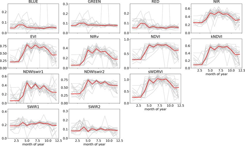
S. Walther et al.: A view from space on global flux towers by MODIS and Landsat                                               2811

  4. Interpolate the remaining gaps with cubic polynomials,         tential non-linear dependencies. We input all MODIS (Land-
     or nearest neighbour in case of very low data availabil-       sat) variables per site together with the information on snow
     ity (fewer than 300 valid data points in the entire time       fraction and the day of year or month of year for MODIS or
     series).                                                       Landsat, respectively. Hence, per site and mission, missFor-
                                                                    est iteratively imputes all variables collectively.
  5. Missing values at the beginning and the end of the
     record cannot be meaningfully filled by temporal meth-         3.3.2    Comparison with other gap-filled data sets:
     ods and are therefore simply repeated.                                  Moreno-Martínez et al. (2020)
Steps 3–5 produced very smooth and, therefore, less realis-         A complementary and mandatory approach to assessing the
tic LST estimates than steps 1–2. Also, one needs to be aware       quality and characteristics of the proposed pre-processing
that any LST estimate in data gaps from this procedure neces-       steps is a comparison against independent data sets and ap-
sarily represents an LST estimate under clear-sky conditions,       proaches (e.g. Moreno-Martínez et al., 2020; Robinson et al.,
which can be very different from the real LST under overcast        2017; Sun et al., 2017). Different spatio-temporal resolutions
skies (Ermida et al., 2019). This needs to be considered for        in the provided data sets and the fact that often mass down-
a given application to prevent the effects of clear-sky bias in     loads of data are necessary to evaluate them at the site level
the LST data sets on the results. Like the vegetation indices,      challenge this approach. However, Moreno-Martínez et al.
LST data layers have a gap-fill flag in FluxnetEO describ-          (2020) provide their gap-filled Landsat surface reflectance at
ing which data points are original and which gap-filling step       the same spatio-temporal resolution as FluxnetEO, and ac-
filled the missing values.                                          cess and cutout at the site level via GEE are feasible. We,
                                                                    therefore, compare the FluxnetEO Landsat product and the
3.3     Evaluation and benchmarking
                                                                    Moreno-Martínez et al. (2020) surface reflectance at 86 sites
                                                                    in the CONUS for the years 2009–2017, which corresponds
3.3.1    FluxnetEO performance in comparison to a
                                                                    to the spatiotemporal domain in which both are available.
         machine learning approach (missForest)
                                                                    In the comparison, we do not differentiate between original
A common approach to benchmarking gap-filling methods is            good-quality and gap-filled estimates because quality con-
to artificially remove samples at positions where the true data     trol and, therefore, gap structure differ between the products.
value is known and then subject the time series to the gap-         However, unphysical reflectance values lower than 0 or larger
filling approach and compare the gap-filled estimates with          than 1 occur, especially in winter, and were removed before
the original values (Moreno-Martínez et al., 2020; Zhang            the cross-consistency analysis, from both good-quality and
et al., 2021; van Buttlar et al., 2014; Wang et al., 2012; Verger   gap-filled estimates.
et al., 2011, 2013; Gerber et al., 2018). We apply this ap-
proach to FluxnetEO in artificial gaps for MODIS and Land-
                                                                    4     Results and discussion
sat variables and randomly remove 20 % and 40 % of data
samples (corresponding to a low and medium gap fraction;            4.1     Gap statistics across indices
compare Fig. 1) per site at positions with originally good
quality. We remove data points from a gap-free time series;         Data availability after quality screening is highly variable be-
i.e. the data points which had been gap-filled before guide         tween sites and depends on the data stream (Fig. 1). Large
the gap filling in the artificial gaps. We feed the time series     differences in the amount of good-quality data in groups of
of the station pixel with artificial gaps into the gap-filling      different climate regions, especially for the reflectances, mir-
approaches described in Sect. 3 and quantify the gap-filling        ror general atmospheric conditions in different regions. Dif-
performance compared to the true values with the Nash–              ferences between spectral bands and reflectance-based in-
Sutcliffe efficiency (NSE, Nash and Sutcliffe, 1970). NSE           dices are very minor in both MODIS and Landsat. MODIS
close to 1 indicates good performance, while negative values        LST generally has fewer valid data points among the data sets
mean worse performance than inputting the simple average            than the reflectance-based indicators, and often fewer during
into the gaps. Decidedly, the NSE refers exclusively to the         daytime than nighttime. While the LSTs are instantaneous
data samples from the artificial gaps and not to the complete       values, the reflectances represent averages over 16 d periods.
time series.                                                        A lower number of good-quality observations in indices that
    To have an independent benchmark of FluxnetEO, we               rely on band 6 relate to degraded detectors in Aqua MODIS
compare to the performance of a versatile imputation                band 6.
method, missForests (Stekhoven and Bühlmann, 2011), in
the same artificial gaps. MissForest is based on random             4.2     Temporal patterns of the gap-filled time series
forests and can handle variables of different types and di-
mensions. It is a multi-output machine learning method that         We illustrate some characteristics of the time series in
iteratively fills gaps across variables, considering their po-      FluxnetEO using the pixel containing an EC station at ex-

https://doi.org/10.5194/bg-19-2805-2022                                                     Biogeosciences, 19, 2805–2840, 2022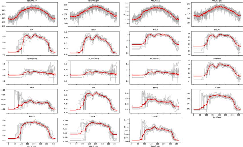
S. Walther et al.: A view from space on global flux towers by MODIS and Landsat
https://doi.org/10.5194/bg-19-2805-2022
Table 2. Data sets presented in FluxnetEO bx refer to the spectral bands. Each data set spans the time period 2000–2020 (MODIS) and 1984–2017 (Landsat) and contains a flag
describing whether a data point is good quality or whether and how it has been estimated in the gap-filling procedures.
Index/variable MODIS Landsat 4, 5, and 7 Landsat 8 Notes
reflectance-based indicators
EVI b2−b1
2.5 · b2+6·b1−7.5·b3+1 b4−b3
2.5 · b4+6·b3−7.5·b1+1 b5−b4
2.5 · b5+6·b4−7.5·b2+1 Huete et al. (2002)
NDVI b2−b1 b4−b3 b5−b4 Tucker (1979)
b2+b1 b4+b3 b5+b4
kNDVI tanh( b2−b1 b2−b1
b2+b1 · b2+b1 ) tanh( b4−b3 b4−b3
b4+b3 · b4+b3 ) tanh( b5−b4 b5−b4
b5+b4 · b5+b4 ) Camps-Valls et al. (2021)
NDWIswir1 b2−b5 b4−b5 b5−b6 Gao (1996)
b2+b5 b4+b5 b5+b6
NDWIswir2 b2−b6 b4−b7 b5−b7 Gao (1996)
b2+b6 b4+b7 b5+b7
NDWIswir3 b2−b7 – – Gao (1996)
b2+b7
NIRv (NDVI − 0.08) · b2 (NDVI − 0.08) · b4 (N DV I − 0.08) · b4 Badgley et al. (2017)
b2−b1
(0.3−1)+(0.3+1)· b2+b1 1−0.3
sWDRVI b2−b1 + 1+0.3 Gitelson (2004)
(0.3+1)+(0.3−1)· b2+b1
RED b1 b3 (RED) b4 (RED)
NIR b2 b4 (NIR) b5 (NIR)
BLUE b3 b1 (BLUE) b2 (BLUE)
GREEN b4 b2 (GREEN) b3 (GREEN)
SWIR1 b5 b5 (SWIR1) –
SWIR2 b6 – b6 (SWIR1)
SWIR3 b7 b7 (SWIR2) b7 (SWIR2)
Biogeosciences, 19, 2805–2840, 2022
MODIS land surface temperature
LST TERRAday , TERRAnight , AQUAday , AQUAnight Each with variable viewing zenith angle
LST_nadir TERRAday , TERRAnight , AQUAday , AQUAnight Corrected to viewing zenith angle = 0◦
LST_oblique TERRAday , TERRAnight , AQUAday , AQUAnight Corrected to viewing zenith angle = 40◦
2812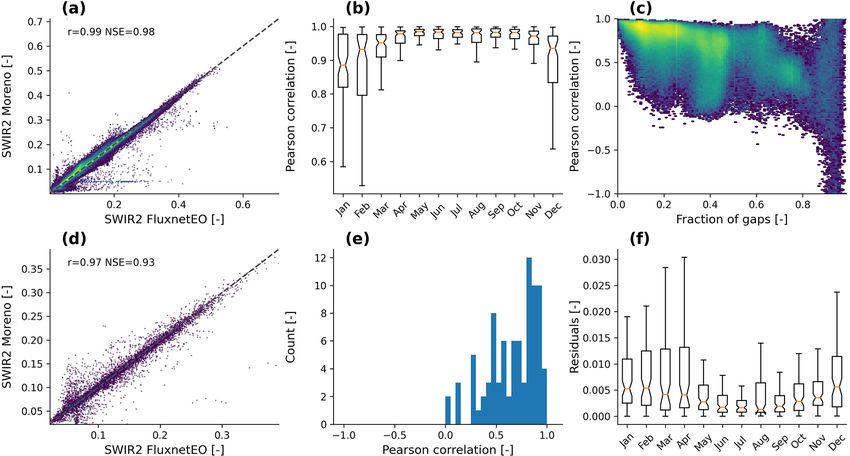
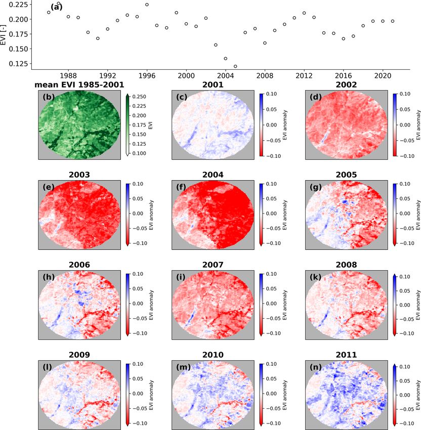
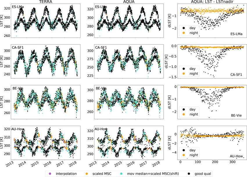
S. Walther et al.: A view from space on global flux towers by MODIS and Landsat                                                  2813

Figure 1. Fraction of good-quality data in the MODIS (a) and Landsat (b) time series. Colours represent the median data availability in
tower pixels across sites grouped by Köppen climate classification. Data refer to the period 2003–2020 for MODIS (the time period when
both Terra and Aqua satellites are in space) and 1990–2017 for Landsat.

ample sites. The Austrian site Neustift (AT-Neu) was situ-            filling unsuccessful at Tharandt in the 1980s, 1994–1995, and
ated in a valley in the Alps and surrounded by grasslands             2008–2012, and in Lonzée a clear seasonality in EVI estab-
which were typically mown three times a year (Wohlfahrt               lishes only after 2000. In addition, for MODIS false filling
et al., 2008). According to their nature, the MODIS LST               by the snow baseline value during the growing season could
time series exhibit faster variability than the vegetation in-        not entirely be prevented, causing an unrealistic dip in one
dices (Fig. 2). Midday observations (AQUAday ) partly show            year in each of the sites. Note that the snow flag contains
an LST increase after the first harvest event in a year around        partly long data gaps in CA-SF1, DE-Tha, and BE-Lon. Fi-
the 150th day of the year. The MSC of most vegetation in-             nally, the woody savanna site Adelaide River (AU-Ade) is a
dices clearly marks the mowing timing, although the relative          typical example of EC sites in climates with a dry and a wet
magnitude varies between indices. Constant values in win-             season. While in the dry season basically no data gaps oc-
ter represent snow-covered times. For Landsat, the granular-          cur, cloud coverage in the rainy season is long enough such
ity of temporal patterns is clearly lower due to the monthly          that mainly the last gap-filling steps of a linearly scaled MSC
sampling, but the characteristic management effects are also          and interpolation take effect for MODIS (Fig. 2). Although
visible here (Fig. 3).                                                the scaling of the MSC does not fully succeed in all years
   Focusing on the example of the EVI, other sites illustrate a       to produce smooth transitions between the good-quality data
few characteristics of the gap-filling procedure in more detail       and the gap-filled ones, the interpolation is able to preserve
(Figs. 4, 5): at the evergreen needleleaf forest site El Saler        inter-annual variations in the MODIS EVI.
in Spain (ES-ES1) much data pass the quality control, and                 Missing MODIS LST values were estimated most reliably
mostly short gaps are reliably filled, also in the absence of a       in the gap-filling steps 1–2 (moving median and scaled av-
very regular seasonal cycle in EVI in both MODIS and Land-            erage shift to observations at other overpass times) because
sat. The boreal forest site Saskatchewan (CA-SF1) illustrates         the typical short-term variability in the time series could be
the effect of a disturbance that happened in 2015 (though the         preserved. In the Spanish site Majadas de Tiétar (ES-LMa,
site was operated only until 2006). The gap-filling procedure         Fig. 6 top panel), savanna-type vegetation is prevalent with
adapts to the modified conditions both abruptly when the dis-         a dry summer and wet winter. Visually the gap-filling proce-
turbance happens and gradually during recovery in the fol-            dure succeeds in preserving the typical higher LST variabil-
lowing years. There is a problematic group of high MODIS              ity in the dry season and seasonally changing diurnal am-
EVI values during winter 2006/2007. The moving window                 plitudes. Also, in Saskatchewan (CA-SF1), gap-filling step 2
outlier filter applied to the MODIS reflectances is by design         successfully estimates the largest fraction of missing values
unable to detect those outliers as they occur consecutively in        for each data stream from the complementary observation
a short period of time. Tharandt (DE-Tha, evergreen needle-           times. The EVI indicated a disturbance event at the begin-
leaf forest) and Lonzée (BE-Lon, crops) are examples of               ning of 2015 (Fig. 4) that continued to strongly affect the
the challenges that data-scarce periods bring for both Land-          EVI also in the following year. The event also marks the LST
sat and MODIS. For MODIS, estimated values in the years               time series in that daytime LST, and therefore, the diurnal
2000–2002 (where only Terra was in operation) are less reli-          amplitude clearly increases in summer after 2015. The gap-
able at both sites. Landsat is particularly scarce and the gap        filling procedure follows this behaviour. Relative to Majadas

https://doi.org/10.5194/bg-19-2805-2022                                                       Biogeosciences, 19, 2805–2840, 2022
2814 S. Walther et al.: A view from space on global flux towers by MODIS and Landsat
Figure 2. Median seasonal cycle (red) and individual yearly trajectories (grey) for MODIS LST (top row) and MODIS vegetation indices
and surface reflectance (second to last rows) in the pixel containing the Austrian site Neustift (AT-Neu). Depending on the data set the central
pixel measures 500 m or 1 km.
de Tiétar or Saskatchewan, in the mixed forest in Vielsalm 4.3 Benchmarking
(BE-Vie), data gaps are much more persistent throughout a
day, and the gap filling works more often with the third gap- In the experiments where artificial gaps are introduced at
filling step using an average seasonal cycle of LST to esti- data points with known and valid values in the pixel con-
mate missing observations. Finally, at the woody savanna site taining the eddy-covariance site, FluxnetEO performance for
Howard Springs in northern Australia (AU-How, Fig. 6 bot- MODIS is excellent with NSE values clearly above 0.9 for
tom panel) there is a strong seasonal phasing between day- all reflectance-based indices, and even above 0.95 for arti-
time and nighttime LST. Data availability also changes with ficial gap fractions of 20 % (Fig. C1 top left). The NSE of
the seasons. In the monsoon season, synoptic variability in the gap-fill estimates for LST is systematically lower but
the filled data points is unrealistically low because the gap- above 0.8 and therefore still very good. Interestingly, the me-
filling needs to resort to filling by a median seasonal cycle of dian NSE across sites is very similar for the 20 % and 40 %
LST (obtained from those years in which the monsoon starts gap fraction experiments for the LST but clearly different for
late) or by interpolation. the reflectance. Overall, FluxnetEO outperforms missForest
Geometrical corrections to the nadir viewing angle are in the realism of the gap-fill estimates slightly but consis-
much larger and have a stronger seasonality for daytime LST tently across most reflectance-based MODIS variables, and
than for nighttime observations (rightmost panel in Fig. 6, more strongly so for the larger (and more realistic for the
Ermida et al., 2018). The daytime LST value from a nadir majority of sites) artificial gap fraction of 40 % (Fig. 7a).
view is consistently estimated to be several kelvin higher The NDWI variables are a special case, where missForest
than from an oblique view. The Australian Howard Springs does not succeed in producing reliable estimates (Fig. C1b)
site is an exception in that the correction offset to nadir has and interestingly more so for low fractions of missing data.
no consistent sign during the wet season. For LST, the ranking between missForest and FluxnetEO
gap filling depends on the gap fraction: missForest consis-
tently produces higher NSE for the lower gap fractions and
FluxnetEO for 40 % of samples removed (Fig. 7a). For Land-
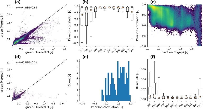
Biogeosciences, 19, 2805–2840, 2022 https://doi.org/10.5194/bg-19-2805-2022S. Walther et al.: A view from space on global flux towers by MODIS and Landsat 2815 Figure 3. Median seasonal cycle (red) and individual yearly trajectories (grey) of the different data sets in the 30 m pixel containing the Austrian site Neustift (AT-Neu) Landsat. sat, the NSE of the gap-fill estimates in FluxnetEO is gen- consistency in both spatial and temporal patterns happen out- erally comparable to (derived vegetation indices) or better side the growing season (DJF in large parts of the CONUS, (spectral bands) than from missForest (Fig. 7b). The perfor- panels b, d, f). This can be expected as NIR reflectance is mance of FluxnetEO is more sensitive to the number of miss- low during this time of the year, and because the treatment ing values than missForest (Fig. C1c, d). A few more points of snow and clouds differs between the products (see time are of note: for both MODIS and Landsat, the gap-fill es- series of one example site in Fig. C8). The temporal cor- timates of spectral surface reflectance in the visible range relation of the deviations from the mean seasonality has a (blue, green, red) are less reliable than the one in channels bimodal pattern with partly low Pearson correlations of un- with longer wavelength or derived vegetation indices. The der 0.5 (panel e). The consistency between FluxnetEO and overall gap-fill performance is not satisfactory for Landsat, Moreno-Martínez et al. (2020) surface reflectance products either from FluxnetEO or from missForest. We did additional generally increases with wavelength, with the lowest agree- tests and found that the signal-to-noise ratio and the temporal ment for the blue spectral band (Figs. C3, C4, C5, C6, C7). resolution are decisive for the success of the gap filling. The These benchmarking exercises illustrate important short- time series of the average across all subpixels in the Land- comings but at the same time clearly support the quality sat cutout exhibit less noise than the time series of the centre of the gap-filling approach proposed by FluxnetEO as be- pixel, which also clearly increases the NSE of the artificial ing comparable to or slightly higher than independent ap- gap-fill estimates (Fig. C2a). FluxnetEO generally performs proaches and products. The artificial gaps at random posi- better on daily than on monthly data (see the lower NSE for tions in the first experiment might be comparable to those ex- MODIS at monthly resolution in Fig. C2b), which calls for pected from bad inversion or clouds. Removing longer con- attempts to improve the reliability of FluxnetEO at different secutive periods such as during snow periods or persistent temporal resolutions in future releases. cloud cover in rainy seasons is not feasible due to limited Figure 8 compares the spatial and temporal patterns consecutive good-quality data, so we cannot test the per- of Landsat NIR reflectance from FluxnetEO and Moreno- formance for gaps of this type. Compared to missForest, Martínez et al. (2020) across sites and shows a high con- FluxnetEO has the great advantage of being easily scalable to sistency (panels a, b, d). The largest differences and lowest large-scale gridded data products. Compared to the product https://doi.org/10.5194/bg-19-2805-2022 Biogeosciences, 19, 2805–2840, 2022
2816                                       S. Walther et al.: A view from space on global flux towers by MODIS and Landsat

Figure 4. Illustration of gap-filling steps in the 500 m pixel containing selected eddy-covariance sites for the MODIS EVI.

Figure 5. Illustration of gap-filling steps in the 30 m pixel containing selected eddy-covariance sites for the Landsat EVI.

Biogeosciences, 19, 2805–2840, 2022                                                            https://doi.org/10.5194/bg-19-2805-2022
S. Walther et al.: A view from space on global flux towers by MODIS and Landsat                                                  2817

Figure 6. MODIS LST gap-filling steps in the 1 km pixel containing selected eddy-covariance sites for daytime and nighttime LST. The
rightmost column shows the average annual cycle of the correction factor between LST from variable viewing angles and LST corrected to
nadir view.

of Moreno-Martínez et al. (2020) FluxnetEO offers coverage           2013), and model–data integration (Williams et al., 2009).
at global sites and is not restricted to the CONUS but lacks         The role that the scale mismatch between site-level and EO
the availability of gridded data.                                    data plays for ecosystem analyses clearly depends on the
                                                                     site and the application. Some applications try to account for
4.4   On the importance of spatial context                           the mismatch (Pacheco-Labrador et al., 2017; Wagle et al.,
                                                                     2020); others ignore it and use a custom area around each
In this section, we present different examples of the relevance      EC site. Approaches to quantify and account for heterogene-
of spatial context. The type and distribution of the vegeta-         ity within a satellite pixel or a certain area around a given site
tion around a given EC measurement station are not neces-            do exist in the literature (Romá et al., 2009; Chu et al., 2021;
sarily homogeneous. Instead, clusters of different vegetation        Duveiller et al., 2021) but seem less exploited.
or land use types might prevail in different sections of the            We computed the average flux footprints for every day
immediate surroundings of a site. The area that a given flux         (MODIS) and month (Landsat) around three example EC sta-
measurement is representative of (the flux footprint, Schmid,        tions (Majadas de Tiétar, ES-LM1, Gebesee, DE-Geb, and
1997) changes rapidly with wind direction, turbulence condi-         Zotino, RU-Zo2). We illustrate how the relationship between
tions, atmospheric stability, and surface resistance (Schmid,        EC-derived gross primary productivity (GPP) and EVI as an
1997; Vesala et al., 2008; Chu et al., 2021). An exact match         EO-derived proxy of the same changes according to whether
between the flux footprint and EO data (or a model grid cell)        the footprint area is taken into account or custom cutout sizes
is challenging due to the often unknown or uncertain flux            are chosen. In RU-Zo2, we compare surface temperature in-
footprints and coarse spatial grid sizes. The scale mismatch is      verted from sensible heat flux to LST and illustrate how the
equally important for validation exercises for site-level mea-       pixel sizes relate to the flux footprint area (see details on the
surements of surface reflectance (Romá et al., 2009; Cescatti        data processing in Appendix D).
et al., 2012), site-level energy-balance closure (Stoy et al.,

https://doi.org/10.5194/bg-19-2805-2022                                                      Biogeosciences, 19, 2805–2840, 2022
2818 S. Walther et al.: A view from space on global flux towers by MODIS and Landsat Figure 7. Benchmarking in artificial gaps: distribution of NSE per site of the gap-fill estimates in artificial gaps by FluxnetEO compared to missForest within the physical ranges of the indices for 20 % and 40 % of good-quality data removed. For MODIS (a) and Landsat (b), random good-quality samples are removed from the tower pixel. The site ES-LM1 (El-Madany et al., 2018) is a tree–grass (Fig. 9a,c). The agricultural areas contribute to fex, while the ecosystem. While the trees are evergreen, the herbaceous footprint intersection methods (fpa and fpw) and the centre layer senesces in summer and re-greens in autumn (Luo et al., pixel (cpx) EVI consistently indicate high greenness in the 2018). The EO cutout includes irrigated agricultural areas tree–grass ecosystem. north of the flux footprint. These fields are barren in winter Gebesee, DE-Geb, is an agricultural site. The common ap- and are covered with crops in summer. MODIS and Landsat proach in conducting EC measurements is to put the tower in EVI are strongly negatively correlated to GPP derived from a location where the land use is as homogeneous as possible, EC in the pixels over agricultural areas, as are the anoma- to be able to attribute fluxes to a targeted ecosystem, e.g. a lies of EVI and GPP (Fig. D1a–d). Conversely, high positive known crop type. In Gebesee, this was assured for most of correlations prevail across the remaining larger parts of the the years in the long site history (e.g. Fig. 9h), but not from EO cutouts. Landsat EVI overlaid by the average flux foot- 2011–2013. In these years, the field was split into two dif- print for two example months illustrates that the EC GPP ferent adjacent crop types that contributed to the measured is only representative of the tree–grass ecosystem (Fig. 9e, fluxes (Fig. 9f), raising the risk for pitfalls in the analyses g). Hence, the spatial representativeness of EO data for EC of the fluxes. Also, in situations/years when the flux foot- fluxes might differ strongly depending on which satellite pix- print represents a single field, additional potential difficul- els are chosen for the analysis. We computed the average ties originate from phenological differences between fields EVI that is representative of the flux footprint (henceforth within the EO cutouts (Fig. 9f, h) if not properly matched. fpa for footprint area). We compared it with an average EVI For example, the anomalies of both GPP and EVI are only weighted with the probability density function of the flux highly correlated with each other in the immediate surround- footprint in order to take into account the decreasing influ- ings of the tower (Fig. D1g–h). Phenological heterogeneity ence of subpixels further away from the tower (henceforth between fields might explain why the EVI averaged over the fpw for weighted footprint area), as well as with two prag- full cutout (fex) is clearly different from the EVI in the foot- matic approaches in case a flux footprint is unknown: an EVI print area (fpa, fpw) or the tower pixel (cpx) during the grow- average over all subpixels in the cutout with a radius of 2 km ing season maxima in 2015/2016 (Fig. 9b, d). Also, con- (henceforth fex for full extent) or only the single subpixel that sistent with the GPP, the EVI in the tower pixel indicates contains the tower (cpx for centre pixel). The most noticeable slightly later senescence in 2017 than averaged over the foot- difference between the time series for the different intersec- print area or the full cutout, highlighting considerable effects tion methods is that the full extent (fex) in both Landsat and of a mismatch between the flux footprint and the EO area. MODIS EVI is comparatively lower during the winter period Biogeosciences, 19, 2805–2840, 2022 https://doi.org/10.5194/bg-19-2805-2022
You can also read